Computing Clusters of Correlation Connected Objects

(1)

Computing Clusters of Correlation Connected Objects

∗

Christian B ¨ohm, Karin Kailing, Peer Kr ¨oger, Arthur Zimek

Institute for Computer Science University of Munich

Oettingenstr. 67, 80538 Munich, Germany

{boehm,kailing,kriegel,kroegerp,zimek}@dbs.informatik.uni-muenchen.de

ABSTRACT

The detection of correlations between different features in a set of feature vectors is a very important data mining task because correlation indicates a dependency between the fea-tures or some association of cause and effect between them. This association can be arbitrarily complex, i.e. one or more features might be dependent from a combination of several other features. Well-known methods like the principal com-ponents analysis (PCA) can perfectly find correlations which are global, linear, not hidden in a set of noise vectors, and uniform, i.e. the same type of correlation is exhibited in all feature vectors. In many applications such as medical diagnosis, molecular biology, time sequences, or electronic commerce, however, correlations are not global since the dependency between features can be different in different subgroups of the set. In this paper, we propose a method called4C (Computing Correlation Connected Clusters) to identify local subgroups of the data objects sharing a uni-form but arbitrarily complex correlation. Our algorithm is based on a combination of PCA and density-based cluster-ing (DBSCAN). Our method has a determinate result and is robust against noise. A broad comparative evaluation demonstrates the superior performance of 4C over compet-ing methods such as DBSCAN, CLIQUE and ORCLUS.

1. INTRODUCTION

The tremendous amount of data produced nowadays in various application domains can only be fully exploited by efficient and effective data mining tools. One of the primary data mining tasks is clustering, which aims at partitioning the objects (described by points in a high dimensional fea-∗_{Supported in part by the German Ministry for Education,} Science, Research and Technology (BMBF) under grant no. 031U112F within the BFAM (Bioinformatics for the Func-tional Analysis of Mammalian Genomes) project which is part of the German Genome Analysis Network (NGFN).

Permission to make digital or hard copies of all or part of this work for personal or classroom use is granted without fee provided that copies are not made or distributed for profit or commercial advantage and that copies bear this notice and the full citation on the first page. To copy otherwise, to republish, to post on servers or to redistribute to lists, requires prior specific permission and/or a fee.

SIGMOD 2004, June 13-18, 2004, Paris, France.

ture space) of a data set into dense regions (clusters) sepa-rated by regions with low density (noise). Knowing the clus-ter structure is important and valuable because the differ-ent clusters often represdiffer-ent differdiffer-ent classes of objects which have previously been unknown. Therefore, the clusters bring additional insight about the stored data set which can be exploited for various purposes such as improved marketing by customer segmentation, determination of homogeneous groups of web users through clustering of web logs, struc-turing large amounts of text documents by hierarchical clus-tering, or developing thematic maps from satellite images.

An interesting second kind of hidden information that may be interesting to users are correlations in a data set. A correlation is a linear dependency between two or more features (attributes) of the data set. The most important method for detecting correlations is the principal compo-nents analysis (PCA) also known as Karhunen Lo`ewe trans-formation. Knowing correlations is also important and valu-able because the dimensionality of the data set can be con-siderably reduced which improves both the performance of similarity search and data mining as well as the accuracy. Moreover, knowing about the existence of a relationship be-tween attributes enables one to detect hidden causalities (e.g. the influence of the age of a patient and the dose rate of medication on the course of his disease or the coregulation of gene expression) or to gain financial advantage (e.g. in stock quota analysis), etc.

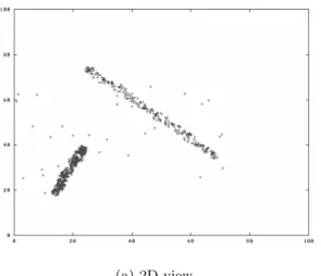
Methods such as PCA, however, are restricted, because they can only be applied to the data set as a whole. There-fore, it is only possible to detect correlations which are ex-pressed in all points or almost all points of the data set. For a lot of applications this is not the case. For instance, in the analysis of gene expression, we are facing the problem that a dependency between two genes does only exist under certain conditions. Therefore, the correlation is visible only in a local subset of the data. Other subsets may be either not correlated at all, or they may exhibit completely differ-ent kinds of correlation (differdiffer-ent features are dependdiffer-ent on each other). The correlation of the whole data set can be weak, even if for local subsets of the data strong correlations exist. Figure 1 shows a simple example, where two subsets of 2-dimensional points exhibit different correlations.

To the best of our knowledge, both concepts of clustering (i.e. finding densely populated subsets of the data) and cor-relation analysis have not yet been addressed as a combined task for data mining. The most relevant related approach is ORCLUS [1], but since it isk-medoid-based, it is very

sen-in Proc. ACM Int. Conf. on Management of Data (SIGMOD), pp. 455-466, Paris, France, 2004

(2)

(a) 2D view.

attribute 1 attribute 2

(b) Transposed view.

Figure 1: 1-Dimensional Correlation Lines

sitive to noise and the locality of the analyzed correlations is usually too coarse, i.e. the number of objects taken into account for correlation analysis is too large (cf. Section 2 and 6 for a detailed discussion). In this paper, we develop a new method which is capable of detecting local subsets of the data which exhibit strong correlations and which are densely populated (w.r.t. a given density threshold). We call such a subset acorrelation connected cluster.

In lots of applications such correlation connected clusters are interesting. For example in E-commerce (recommenda-tion systems or target marketing) where sets of customers with similar behavior need to be detected, one searches for positive linear correlations. In DNA microarray analysis (gene expression analysis) negative linear correlations ex-press the fact that two genes may be coregulated, i.e. if one has a high expression level, the other one is very low and

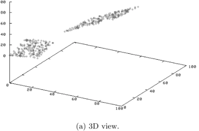
vice versa. Usually such a coregulation will only exist in a small subset of conditions or cases, i.e. the correlation will be hidden locally in the data set and cannot be detected by global techniques. Figures 1 and 2 show simple examples how correlation connected clusters can look like. In Figure 1 the attributes exhibit two different forms of linear corre-lation. We observe that if for some points there is a linear correlation of all attributes, these points are located along a line. Figure 2 presents two examples where an attributez

is correlated to attributesxandy(i.e. z=a+bx+cy). In this case the set of points forms a 2-dimensional plane.

As stated above, in this paper, we propose an approach that meets both the goal of clustering and correlation anal-ysis in order to find correlation connected clusters. The remainder is organized as follows: In Section 2 we review and discuss related work. In Section 3 we formalize our notion of correlation connected clusters. Based on this for-malization, we present in Section 4 an algorithm called 4C (ComputingCorrelationConnectedClusters) to efficiently compute such correlation connected clusters. In Section 5 we analyze the computational complexity of our algorithm, while Section 6 contains an extensive experimental evalua-tion of 4C. Secevalua-tion 7 concludes the paper and gives some hints at future work.

2. RELATED WORK

Traditional clustering algorithms such ask-means or the EM-algorithm search for spatial clusters, which are spher-ically shaped. In [10] and [5] two algorithms are proposed which are able to find clusters of arbitrary shape. However, these approaches are not able to distinguish between arbi-trarily shaped clusters and correlation clusters. In [10] the density-based algorithm DBSCAN is introduced. We will describe the basic concepts of this approach in detail in the next chapter. In [5] the authors propose the algorithm FC (Fractal Clustering) to find clusters of arbitrary shape. The paper presents only experiments for two-dimensional data sets, so it is not clear whether the fractal dimension is re-ally stable in higher dimensions. Furthermore, the shapes of clusters depend on the type of correlation of the involved points. Thus, in the case of linear correlations it is more target-oriented to search for shapes like lines or hyperplanes than for arbitrarily shaped clusters.

As most traditional clustering algorithms fail to detect meaningful clusters in high-dimensional data, in the last years a lot of research has been done in the area of sub-space clustering. In the following we are examining to what extent subspace clustering algorithms are able to capture lo-cal data correlations and find clusters of correlated objects. The principal axis of correlated data are arbitrarily oriented. In contrast, subspace clustering techniques like CLIQUE [3] and its successors MAFIA [11] or ENCLUS [9] or projected clustering algorithms like PROCLUS [2] and DOC [17] only find axis parallel projections of the data. In the evaluation part we show that CLIQUE as one representative algorithm is in fact not able to find correlation clusters. Therefore we focus our attention to ORCLUS [1] which is ak-medoid related projected clustering algorithm allowing clusters to exist in arbitrarily oriented subspaces. The problem of this approach is that the user has to specify the number of clus-ters in advance. If this guess does not correspond to the actual number of clusters the results of ORCLUS deterio-rate. A second problem, which can also be seen in the eval-uation part is noisy data. In this case the clusters found by ORCLUS are far from optimal, since ORCLUS assigns each object to a cluster and thus cannot handle noise efficiently.

(3)

(a) 3D view.

attribute 1 attribute 2 attribute 3

(b) Transposed view of one plane.

Figure 2: 2-Dimensional Correlation Planes

Based on the fractal (intrinsic) dimensionality of a data set, the authors of [15] present a global dimensionality re-duction method. Correlation in the data leads to the phe-nomenon that the embedding dimension of a data set (in other words the number of attributes of the data set) and the intrinsic dimension (the dimension of the spatial ob-ject represented by the data) can differ a lot. The intrin-sic (correlation fractal dimension) is used to reduce the di-mensionality of the data. As this approach adopts a global view on the data set and does not account for local data distributions, it cannot capture local subspace correlations. Therefore it is only useful and applicable, if the underly-ing correlation affects all data objects. Since this is not the case for most real-world data, in [8] a local dimensionality reduction technique for correlated data is proposed which is similar to [1]. The authors focus on identifying correlated clusters for enhancing the indexing of high dimensional data only. Unfortunately, they do not give any hint to what ex-tent their heuristic-based algorithm can also be used to gain new insight into the correlations contained in the data.

In [23] the move-based algorithm FLOC computing near-optimal δ-clusters is presented. A transposed view of the data is used to show the correlations which are captured by theδ-cluster model. Each data object is shown as a curve where the attribute values of each object are connected. Ex-amples can be seen in Figure 1(b) and 2(b). A cluster is regarded as a subset of objects and attributes for which the participating objects show the same (or a similar) tendency rather than being close to each other on the associated sub-set of dimensions. Theδ-cluster model concentrates on two forms of coherence, namely shifting (or addition) and am-plification (or production). In the case of amam-plification co-herence for example, the vectors representing the objects must be multiples of each other. The authors state that this can easily be transformed to the problem of finding shift-ing coherent δ-cluster by applying logarithmic function to each object. Thus they focus on finding shifting coherentδ -clusters and introduce the metric of residue to measure the coherency among objects of a given cluster. An advantage is that thereby they can easily handle missing attribute val-ues. But in contrast to our approach, theδ-cluster model limits itself to a very special form of correlation where all at-tributes are positively linear correlated. It does not include

negative correlations or correlations where one attribute is determined by two or more other attributes. In this cases searching for a trend is no longer possible as can be seen in Figure 1 and 2. Let us note, that such complex dependen-cies cannot be illustrated by transposed views of the data. The same considerations apply for the very similar p-cluster model introduced in [21] and two extensions presented in [16, 14].

3. THE NOTION OF CORRELATION

CON-NECTED CLUSTERS

In this section, we formalize the notion of a correlation connected cluster. Let D be a database of d-dimensional feature vectors (D ⊆Rd

). An elementP ∈ Dis called point or object. The value of the i-th attribute (1 _≤ i_≤ d) of

P is denoted by pi (i.e. P = (p1, . . . , pd)T). Intuitively, a

correlation connected cluster is a dense region of points in thed-dimensional feature space having at least one principal axis with low variation along this axis. Thus, a correlation connected cluster has two different properties: density and correlation. In the following, we will first address these two properties and then merge these ingredients to formalize our notion of correlation connected clusters.

3.1 Density-Connected Sets

The density-based notion is a common approach for clus-tering used by various clusclus-tering algorithms such as DB-SCAN [10], DBCLASD [22], DENCLUE [12], and OPTICS [4]. All these methods search for regions of high density in a feature space that are separated by regions of lower density. A typical density-based clustering algorithm needs two pa-rameters to define the notion of density: First, a parameter

µ specifying the minimum number of objects, and second, a parameterε specifying a volume. These two parameters determine a density threshold for clustering.

Our approach follows the formal definitions of density-based clusters underlying the algorithm DBSCAN. The for-mal definition of the clustering notion is presented and dis-cussed in full details in [10]. In the following we give a short summary of all necessary definitions.

Definition 1 (ε-neighborhood).

(4)

by_Nε(O), is defined by

Nε(O) ={X∈ D |dist(O, X)≤ε}.

Based on the two input parametersεandµ, dense regions can be defined by means of core objects:

Definition 2 (core object).

Let ε ∈ R and µ ∈ N. An object O ∈ D is called core objectw.r.t. εandµ, if itsε-neighborhood contains at least

µobjects, formally:

Coreden(O)⇔ | Nε(O)| ≥µ.

Let us note, that we use the acronym “den” for the density parametersε andµ. In the following, we omit the param-etersε and µwherever the context is clear and use “den” instead.

A core objectOcan be used to expand a cluster, with all the density-connected objects of O. To find these objects the following concepts are used.

Definition 3 (direct density-reachability). Letε_∈Randµ_∈N. An objectP _{∈ D}isdirectly density-reachable fromQ∈ D w.r.t. ε andµ, if Qis a core object andP is an element ofNε(Q), formally:

DirReachden(Q, P)⇔Coreden(Q) ∧ P ∈ Nε(Q).

Let us note, that direct density-reachability is symmetric only for core objects.

Definition 4 (density-reachability).

Letε_∈Randµ_∈N. An objectP_{∈ D}isdensity-reachable

fromQ ∈ D w.r.t. ε and µ, if there is a chain of objects P1, . . . ,Pn∈ D, P1=Q,Pn=P such thatPi+1 is directly

density-reachable fromPi, formally:

Reachden(Q, P)⇔

∃P1, . . . ,Pn∈ D :P1=Q ∧ Pn=P ∧

∀i∈ {1, . . . , n−1} :DirReachden(Pi, Pi+1). Density-reachability is the transitive closure of direct density-reachability. However, it is still not symmetric in general.

Definition 5 (density-connectivity).

Letε∈Randµ∈N. An objectP ∈ Disdensity-connected

to an object Q ∈ D w.r.t. ε and µ, if there is an object

O∈ D such that bothP andQ are density-reachable from

O, formally:

Connectden(Q, P)⇔

∃O∈ D : Reach_den(O, Q) ∧ Reach_den(O, P).

Density-connectivity is a symmetric relation. A density-connected cluster is defined as a set of density-density-connected objects which is maximal w.r.t. density-reachability [10].

Definition 6 (density-connected set).

Let ε ∈ R and µ ∈ N. A non-empty subset C ⊆ D is called adensity-connected setw.r.t. ε andµ, if all objects in_Care density-connected and_C is maximal w.r.t. density-reachability, formally:

ConSet_den(C)⇔

(1) Connectivity: ∀O, Q∈ C:Connectden(O, Q)

(2) Maximality:∀P, Q∈ D:Q∈ C∧Reachden(Q, P)⇒

P ∈ C.

Using these concepts DBSCAN is able to detect arbitrar-ily shaped clusters by one single pass over the data. To do so, DBSCAN uses the fact, that a density-connected cluster can be detected by finding one of its core-objectsOand com-puting all objects which are density reachable fromO. The correctness of DBSCAN can be formally proven (cf. lem-mata 1 and 2 in [10], proofs in [19]). Although DBSCAN is not in a strong sense deterministic (the run of the algo-rithm depends on the order in which the points are stored), both the run-time as well as the result (number of detected clusters and association of core objects to clusters) are de-terminate. The worst case time complexity of DBSCAN is

O(nlogn) assuming an efficient index andO(n2) if no index exists.

3.2 Correlation Sets

In order to identify correlation connected clusters (regions in which the points exhibit correlation) and to distinguish them from usual clusters (regions of high point density only) we are interested in all sets of points with an intrinsic di-mensionality that is considerably smaller than the embed-ding dimensionality of the data space (e.g. a line or a plane in a three or higher dimensional space). There are several methods to measure the intrinsic dimensionality of a point set in a region, such as the fractal dimension or the prin-cipal components analysis (PCA). We choose PCA because the fractal dimension appeared to be not stable enough in our first experiments.

The PCA determines the covariance matrix M = [mij]

withmij = P S∈S

sisj of the considered point set S, and

de-composes it into an orthonormal MatrixVcalled eigenvec-tor matrix and a diagonal matrixEcalled eigenvalue matrix such thatM=VEVT_{. The eigenvectors represent the} prin-cipal axes of the data set whereas the eigenvalues represent the variance along these axes. In case of a linear dependency between two or more attributes of the point set (correla-tion), one or more eigenvalues are close to zero. A set forms aλ-dimensional correlation hyperplane ifd−λeigenvalues fall below a given threshold δ _≈ 0. Since the eigenvalues of different sets exhibiting different densities may differ a lot in their absolute values, we normalize the eigenvalues by mapping them onto the interval [0,1]. This normalization is denoted by Ω and simply divides each eigenvalueei by the

maximum eigenvalueemax. We call the eigenvaluesei with

Ω(ei)≤δclose to zero.

Definition 7 (λ-dimensional linear correlation set).

Let S ⊆ D, λ ∈ N (λ ≤ d), EV = e1, ..., ed the

eigen-values ofS in descending order (i.e. ei≥ei+1) and δ∈R (δ ≈ 0). S forms an λ-dimensional linear correlation set

w.r.t. δ if at leastd₋λ eigenvalues of_S are close to zero, formally:

CorSetλδ(S)⇔ |{ei∈EV|Ω(ei)≤δ}| ≥d−λ.

whereΩ(ei) =ei/e1.

This condition states that the variance ofS along d−λ

principal axes is low and therefore the objects ofS form an

λ-dimensional hyperplane. We drop the indexλand speak of a correlation set in the following wherever it is clear from context.

(5)

P major axis of

the data set

(a)

P

/

(b)

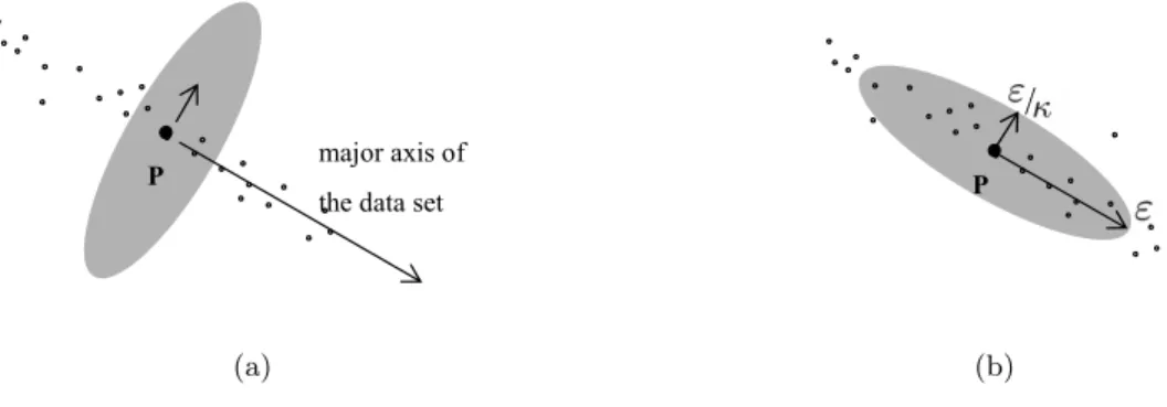
Figure 3: Correlation ε-neighborhood of a point P according to (a) MP and (b) ˆMP.

Definition 8 (Correlation dimension).

Let S ∈ D be a linear correlation set w.r.t. δ ∈ N. The number of eigenvalues withei > δ is called correlation

di-mension, denoted byCorDim(S).

Let us note, that if_Sis aλ-dimensional linear correlation set, thenCorDim(S)≤λ. The correlation dimension of a linear correlation setS corresponds to the intrinsic dimen-sion of_S.

3.3 Clusters as Correlation-Connected Sets

A correlation connected cluster can be regarded as a max-imal set of density-connected points that exhibit uniform correlation. We can formalize the concept of correlation connected sets by merging the concepts described in the pre-vious two subsections: density-connected sets (cf. Definition 6) and correlation sets (cf. Definition 7). The intuition of our formalization is to consider those points as core objects of a cluster which have an appropriate correlation dimension in their neighborhood. Therefore, we associate each pointP

with a similarity matrixMP which is determined by PCA

of the points in theε-neighborhood ofP. For convenience we callVP and EP the eigenvectors and eigenvalues of P,

respectively. A pointP is inserted into a cluster if it has the same or a similar similarity matrix like the points in the cluster. To achieve this goal, our algorithm looks for points that are close to the principal axis (or axes) of those points which are already in the cluster. We will define a similarity measureMˆP for the efficient search of such points.

We start with the formal definition of the covariance ma-trixMP associated with a pointP.

Definition 9 (covariance matrix).

LetP∈ D. The matrixMP = [mij]with

mij=

X

S∈Nε(P)

sisj (1≤i, j≤d)

is called thecovariance matrix of the pointP. VP andEP

(withMP =VPEPVTP) as determined by PCA ofMP are

called the eigenvectors and eigenvalues of the point P, re-spectively.

We can now define the new similarity measureMˆP which

searches points in the direction of highest variance ofMP

(the major axes). Theoretically,MP could be directly used

as a similarity measure, i.e.

distMP(P, Q) = p

(P−Q)MP(P−Q)T whereP, Q∈ D.

Figure 3(a) shows the set of points which lies in an ε -neighborhood of the point usingMP as similarity measure.

The distance measure puts high weights on those axes with a high variance whereas directions with a low variance are associated with low weights. This is usually desired in sim-ilarity search applications where directions of high variance have a high distinguishing power and, in contrast, directions of low variance are negligible.

Obviously, for our purpose of detecting correlation clus-ters, we need quite the opposite. We want so search for points in the direction of highest variance of the data set. Therefore, we need to assign low weights to the direction of highest variance in order to shape the ellipsoid such that it reflects the data distribution (cf. Figure 3(b)). The solu-tion is to change large eigenvalues into smaller ones andvice versa. We use two fixed values, 1 and a parameter κ1 rather than e.g. inverting the eigenvalues in order to avoid problems with singular covariance matrices. The number 1 is a natural choice because the corresponding semi-axes of the ellipsoid are then epsilon. The parameterκcontrols the ”thickness” of the λ-dimensional correlation line or plane, i.e. the tolerated deviation.

This is formally captured in the following definition:

Definition 10 (correlation similarity matrix).

Let P ∈ D and VP, EP the corresponding eigenvectors

and eigenvalues of the point P. Let κ _∈ Rbe a constant withκ1. The new eigenvalue matrix EˆP with entriesˆei

(i= 1, . . . d) is computed from the eigenvaluese1, . . . , ed in

EP according to the following rule:

ˆ

ei=

1 if Ω(ei)> δ

κ if Ω(ei)≤δ

where Ω is the normalization of the eigenvalues onto [0,1]

as described above. The matrix MˆP =VPEˆPVTP is called

thecorrelation similarity matrix. Thecorrelation similarity measureassociated with pointP is denoted by

distP(P, Q) =

q

(P₋Q)_·MˆP·(P−Q)T.

Figure 3(b) shows the ε-neighborhood according to the correlation similarity matrixMˆP. As described above, the

parameter κspecifies how much deviation from the corre-lation is allowed. The greater the parameterκ, the tighter and clearer the correlations which will be computed. It em-pirically turned out that our algorithm presented in Section

(6)

P

Q

P

Q

(a)

P

Q

P

Q

(b)

Figure 4: Symmetry of the correlationε-neighborhood: (a)P ∈ NMˆQ

ε (Q). (b)P6∈ N

ˆ MQ

ε (Q).

4 is rather insensitive to the choice ofκ. A good suggestion is to setκ= 50 in order to achieve satisfying results, thus — for the sake of simplicity — we omit the parameterκin the following.

Using this similarity measure, we can define the notions of correlation core objects and correlation reachability. How-ever, in order to define correlation-connectivity as a symmet-ric relation, we face the problem that the similarity measure in Definition 10 is not symmetric, because distP(P, Q) =

distQ(Q, P) does in general not hold (cf. Figure 4(b)).

Symmetry, however, is important to avoid ambiguity of the clustering result. If an asymmetric similarity measure is used in DBSCAN a different clustering result can be ob-tained depending on the order of processing (e.g. which point is selected as the starting object) because the sym-metry of density-connectivity depends on the symsym-metry of direct density-reachability for core-objects. Although the result is typically not seriously affected by this ambiguity effect we avoid this problem easily by an extension of our similarity measure which makes it symmetric. The trick is to consider both similarity measures,distP(P, Q) as well as

distQ(P, Q) and to combine them by a suitable arithmetic

operation such as the maximum of the two. Based on these considerations, we define the correlationε-neighborhood as a symmetric concept:

Definition 11 (correlationε-neighborhood).

Let ε _∈ R. The correlation ε-neighborhood of an object

O∈ D, denoted byNMˆO

ε (O), is defined by:

NMˆO

ε (O) ={X∈ D |max{distO(O, X), distX(X, O)} ≤ε}.

The symmetry of the correlationε-neighborhood is illus-trated in Figure 4. Correlation core objects can now be defined as follows.

Definition 12 (correlation core object).

Let ε, δ ∈ R and µ, λ ∈ N. A point O ∈ D is called

correlation core object w.r.t. ε, µ, δ, and λ (denoted by Corecorden(O)), if itsε-neighborhood is aλ-dimensional linear

correlation set and its correlationε-neighborhood contains at leastµpoints, formally:

Corecorden(O)⇔CorSet

λ

δ(Nε(P))∧ | N

ˆ M_P

ε (P)| ≥µ.

Let us note that inCorecor_den the acronym “cor” refers to the correlation parameters δ and λ. In the following, we

omit the parametersε,µ,δ, andλwherever the context is clear and use “den” and “cor” instead.

Definition 13 (Direct correlation-reachability).

Let ε, δ ∈ R and µ, λ ∈ N. A point P ∈ D is direct correlation-reachable from a point Q ∈ D w.r.t. ε, µ, δ, andλ(denoted byDirReachcorden(Q,P)) ifQis a correlation

core object, the correlation dimension of Nε(P) is at least

λ, andP ∈ NMˆQ

ε (Q), formally:

DirReachcorden(Q, P)⇔

(1) Corecor_den(Q)

(2) CorDim(Nε(P))≤λ

(3) P∈ NMˆQ

ε (Q).

Correlation-reachability is symmetric for correlation core objects. Both objects P andQmust find the other object in their corresponding correlationε-neighborhood.

Definition 14 (correlation-reachability).

Let ε, δ ∈ R (δ ≈ 0) and µ, λ∈ N. An object P ∈ D is

correlation-reachable from an objectQ∈ D w.r.t. ε, µ, δ, and λ (denoted by Reachcorden(Q,P)), if there is a chain of

objects P1,· · ·Pn such that P1 = Q, Pn = P and Pi+1 is

direct correlation-reachable fromPi, formally:

Reachcorden(Q, P)⇔

∃P1, . . . ,Pn∈ D :P1=Q ∧ Pn=P ∧

∀i∈ {1, . . . , n−1} :DirReachcorden(Pi, Pi+1). It is easy to see, that correlation-reachability is the tran-sitive closure of direct correlation-reachability.

Definition 15 (correlation-connectivity).

Let ε ∈ R and µ ∈ N. An object P ∈ D is correlation-connected to an object Q_{∈ D} if there is an object O_{∈ D}

such that both P and Q are correlation-reachable from O, formally:

Connectcorrden(Q, P)⇔

∃o_{∈ D} : Reachcorrden(O, Q) ∧ Reach corr den(O, P).

Correlation-connectivity is a symmetric relation. A connected cluster can now be defined as a maximal correlation-connected set:

(7)

Definition 16 (correlation-connected set). Letε, δ ∈R andµ, λ∈ N. A non-empty subset C ⊆ D is called a density-connected set w.r.t. ε, µ, δ, and λ, if all objects in_C are density-connected and _C is maximal w.r.t. density-reachability, formally:

ConSetcor_den(C)⇔

(1) Connectivity: _∀O, Q_{∈ C}:Connectcorden(O, Q)

(2) Maximality:∀P, Q∈ D:Q∈ C∧Reachcor_den(Q, P)⇒

P ∈ C.

The following two lemmata are important for validating the correctness of our clustering algorithm. Intuitively, they state that we can discover a correlation-connected set for a given parameter setting in a two-step approach: First, choose an arbitrary correlation core objectOfrom the data-base. Second, retrieve all objects that are correlation-reachable fromO. This approach yields the density-connected set con-tainingO.

Lemma 1.

Let P ∈ D. If P is a correlation core object, then the set of objects, which are correlation-reachable fromP is a correlation-connected set, formally:

Corecorden(P)∧ C={O∈ D |Reachcorden(P, O)} ⇒ConSetcorden(C).

Proof.

(1) C 6=∅:

By assumption,Corecorden(P) and thus, CorDim(Nε(P))≤

λ.

⇒DirReachcor_den(P, P) ⇒Reachcorden(P, P) ⇒P ∈ C.

(2) Maximality:

LetX _{∈ C}andY _{∈ D}andReachcorden(X, Y). ⇒Reachcor_den(P, X)∧Reachcor_den(X, Y)

⇒Reachcor_den(P, Y) (since correlation reachability is a tran-sitive relation).

⇒Y ∈ C.

(3) Connectivity:

∀X, Y _{∈ C}:Reachcorden(P, X)∧Reachcorden(P, Y) ⇒Connectcor_den(X, Y) (viaP).

Lemma 2.

Let _{C ⊆ D} be a correlation-connected set. Let P _{∈ C} be a correlation core object. Then C equals the set of objects which are correlation-reachable fromP, formally:

ConSetcorden(C)∧P∈ C ∧Core cor den(P) ⇒ C={O∈ D |Reachcorden(P, O)}.

Proof.

Let ¯C ={O∈ D |Reachcorden(P, O)}. We have to show that ¯

C=C:

(1) C ⊆ C¯ : obvious from definition of ¯C.

(2) C ⊆ _C¯_{: Let} _Q _{∈ C}_. _{By assumption,} _P _{∈ C} _and

ConSetcor_den(C).

⇒ ∃O∈ C:Reachcorden(O, P)∧Reachcorden(O, Q)

⇒Reachcorden(P, O) (since bothOandPare correlation core objects and correlation reachability is symmetric for corre-lation core objects.

⇒Reachcorden(P, Q) (transitivity of correlation-reachability) ⇒Q∈_C¯_.

algorithm4C(D,ε,µ,λ,δ)

// assumption: each object inDis marked as unclassified for each unclassifiedO∈ Ddo

STEP 1. testCorecor_den(O)predicate: computeNε(O); if|Nε(O)| ≥µthen computeMO; ifCorDim(Nε(O))≤λthen computeMˆOandN ˆ MO ε (O); test|NMˆO ε (O)| ≥µ;

STEP 2.1. if Corecor_den(O)expand a new cluster:

generate new clusterID; insert allX∈ NMˆO

ε (O)into queueΦ;

whileΦ6=∅do

Q= first object inΦ;

computeR={X∈ D |DirReachcor_den(Q, X)}; for eachX∈ Rdo

ifX is unclassified or noisethen assign current clusterID toX

ifX is unclassifiedthen insertX intoΦ; removeQfromΦ;

STEP 2.2. if notCorecor_den(O)Ois noise: markOas noise;

end.

Figure 5: Pseudo code of the 4C algorithm.

4. ALGORITHM 4C

In the following we describe the algorithm 4C, which per-forms one pass over the database to find all correlation clus-ters for a given parameter setting. The pseudocode of the algorithm 4C is given in Figure 5. At the beginning each object is marked as unclassified. During the run of 4C all objects are either assigned a certain cluster identifier or marked as noise. For each object which is not yet classified, 4C checks whether this object is a correlation core object (see STEP 1 in Figure 5). If the object is a correlation core object the algorithm expands the cluster belonging to this object (STEP 2.1). Otherwise the object is marked as noise (STEP 2.2). To find a new cluster 4C starts in STEP 2.1 with an arbitrary correlation core objectOand searches for all objects that are correlation-reachable from O. This is sufficient to find the whole cluster containing the objectO, due to Lemma 2. When 4C enters STEP 2.1 a new cluster identifier “clusterID” is generated which will be assigned to all objects found in STEP 2.1. 4C begins by inserting all objects in the correlationε-neighborhood of objectOinto a queue. For each object in the queue it computes all directly correlation reachable objects and inserts those objects into the queue which are still unclassified. This is repeated until the queue is empty.

As discussed in Section 3 the results of 4C do not depend on the order of processing, i.e. the resulting clustering (num-ber of clusters and association of core objects to clusters) is determinate.

(8)

5. COMPLEXITY ANALYSIS

The computational complexity with respect to the number of data points as well as the dimensionality of the data space is an important issue because the proposed algorithms are typically applied to large data sets of high dimensionality. The idea of our correlation connected clustering method is founded on DBSCAN, a density based clustering algorithm for Euclidean data spaces. The complexity of the original DBSCAN algorithm depends on the existence of an index structure for high dimensional data spaces. The worst case complexity isO(n2), but the existence of an efficient index reduces the complexity toO(nlogn) [10]. DBSCAN is lin-ear in the dimensionality of the data set for the Euclidean distance metric. If a quadratic form distance metric is ap-plied instead of Euclidean (which enables user adaptability of the distance function), the time complexity of DBSCAN isO(d2·nlogn). In contrast, subspace clustering methods such as CLIQUE are known to be exponential in the number of dimensions [1, 3].

We begin our analysis with the assumption of no index structure.

Lemma 3. The overall worst-case time complexity of our algorithm on top of the sequential scan of the data set is

O(d2·n2+d3·n).

Proof. Our algorithm has to associate each point of the

data set with a similarity measure that is used for searching neighbors (cf. Definition 10). We assume that the corre-sponding similarity matrix must be computed once for each point, and it can be held in the cache until it is no more needed (it can be easily decided whether or not the similar-ity matrix can be safely discarded). The covariance matrix is filled with the result of a Euclidean range query which can be evaluated inO(d·n) time. Then the matrix is decom-posed using PCA which requiresO(d3_{) time. For all points} together, we haveO(d·n2₊_d3_·_n_).

Checking the correlation core point property according to Definition 12, and expanding a correlation connected clus-ter requires for each point the evaluation of a range query with a quadratic form distance measure which can be done inO(d2·n). For all points together (including the above cost for the determination of the similarity matrix), we obtain an worst-case time complexity ofO(d2·n2+d3·n).

Under the assumption that an efficient index structure for high dimensional data spaces [7, 6] is available, the complex-ity of all range queries is reduced fromO(n) toO(logn). Let us note that we can use Euclidean range queries as a filter step for the quadratic form range queries because no semi-axis of the corresponding ellipsoid exceedsε. Therefore, the overall time complexity in this case is given as follows:

Lemma 4. The overall worst case time complexity of our algorithm on top of an efficient index structure for high di-mensional data isO(d2_·_n_log_n₊_d3_·_n₎_.

Proof. Analogous to Lemma 3.

6. EVALUATION

In this section, we present a broad evaluation of 4C. We implemented 4C as well as the three comparative methods DBSCAN, CLIQUE, and ORCLUS in JAVA. All experi-ments were run on a Linux workstation with a 2.0 GHz CPU and 2.0 GB RAM.

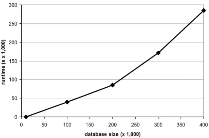
0 50 100 150 200 250 300 0 50 100 150 200 250 300 350 400 database size (x 1,000) ru n ti m e ( s x 1, 000)

Figure 6: Scalability against database size.

6.1 Efficiency

According to Section 5 the runtime of 4C scales super-linear with the number of input records. This is illustrated in Figure 6 showing the results of 4C applied to synthetic 2-dimensional data of variable size.

6.2 Effectiveness

We evaluated the effectiveness of 4C on several synthetic data sets as well as on real world data sets including gene expression data and metabolome data. In addition, we com-pared the quality of the results of our method to the quality of the results of DBSCAN, ORCLUS, and CLIQUE. In all our experiments, we set the parameterκ= 50 as suggested in Section 3.3.

6.2.1 Synthetic Data Sets

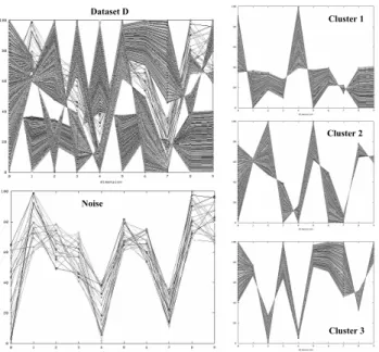
We first applied 4C on several synthetic data sets (with 2≤d≤30) consisting of several dense, linear correlations. In all cases, 4C had no problems to identify the correlation-connected clusters. As an example, Figure 7 illustrates the transposed view of the three clusters and the noise 4C found on a sample 10-dimensional synthetic data set consisting of approximately 1,000 points.

6.2.2 Real World Data Sets

Gene Expression Data. We applied 4C to the gene expression data set of [20]. The data set is derived from time series experiments on the yeast mitotic cell cycle. The expression levels of approximately 3000 genes are measured at 17 different time slots. Thus, we face a 17-dimensional data space to search for correlations indicating coregulated genes. 4C found 60 correlation connected clusters with few coregulated genes (10-20). Such small cluster sizes are quite reasonable from a biological perspective. The transposed views of four sample clusters are depicted in Figure 8. All four clusters exhibit simple linear correlations on a sub-set of their attributes. Let us note, that we also found other linear correlations which are rather complex to visual-ize. We also analyzed the results of our correlation clusters (based on the publicly available information resources on the yeast genome [18]) and found several biologically im-portant implications. For example one cluster consists of several genes coding for proteins related to the assembly of the spindle pole required for mitosis (e.g. KIP1, SLI15, SPC110, SPC25, and NUD1). Another cluster contains

(9)

sev-Dataset D

Cluster 1

Cluster 2

Cluster 3 Noise

Figure 7: Clusters found by 4C on 10D synthetic data set. Parameters: ε= 10.0, µ= 5, λ= 2,δ= 0.1.

eral genes coding for structural constituents of the ribosome (e.g. RPL4B, RPL15A, RPL17B, and RPL39). The func-tional relationships of the genes in the clusters confirm the significance of the computed coregulation.

Metabolome Data. We applied 4C on a metabolome data set [13]. The data set consists of the concentrations of 43 metabolites in 2,000 human newborns. The newborns were labeled according to some specific metabolic diseases. Thus, the data set consists of 2,000 data points with d = 43. 4C detected six correlation connected sets which are visualized in Figure 9. Cluster one and two (in the lower left corner marked with “control”) consists of healthy newborns whereas the other clusters consists of newborns having one specific disease (e.g. “PKU” or “LCHAD”). The group of newborns suffering from “PKU” was split in three clusters. Several ill as well as healthy newborns were classified as noise.

6.2.3 Comparisons to Other Methods

We compared the effectiveness of 4C with related cluster-ing methods, in particular the density-based clustercluster-ing algo-rithm DBSCAN, the subspace clustering algoalgo-rithm CLIQUE, and the projected clustering algorithm ORCLUS. For that purpose, we applied these methods on several synthetic data-sets including 2-dimensional datadata-sets and higher dimensional datasets (d= 10).

Comparison with DBSCAN. The clusters found by DBSCAN and 4C applied on the 2-dimensional data sets are depicted in Figure 10. In both cases, DBSCAN finds clusters which do not exhibit correlations (and thus are not detected by 4C). In addition, DBSCAN cannot distinguish varying correlations which overlap (e.g. both correlations in data set B in Figure 10) and treat such clusters as one density-connected set, whereas 4C can differentiate such cor-relations. We gain similar observations when we applied DB-SCAN and 4C on the higher dimensional data sets. Let us note, that these results are not astonishing since DBSCAN only searches for density connected sets but does not search

Sample Cluster 1 Sample Cluster 2

Sample Cluster 4 Sample Cluster 3

Figure 8: Sample clusters found by 4C on the gene expression data set. Parameters: ε = 25.0, µ = 8,

λ= 8,δ= 0.01.

for correlations and thus cannot be applied to the task of finding correlation connected sets.

Comparison with CLIQUE. A comparison of 4C with CLIQUE gained similar results. CLIQUE finds clusters in subspaces which do not exhibit correlations (and thus are not detected by 4C). On the other hand, CLIQUE is usually limited to axis-parallel clusters and thus cannot detect arbi-trary correlations. These observations occur especially with higher dimensional data (d≥10 in our tests). Again, these results are not astonishing since CLIQUE only searches for axis-parallel subspace clusters (dense projections) but does not search for correlations. This empirically supported the suspicion that CLIQUE cannot be applied to the task of finding correlation connected sets.

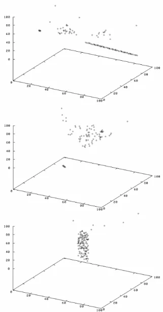
Comparison with ORCLUS. A comparison of 4C with ORCLUS resulted in quite different observations. In fact, ORCLUS computes clusters of correlated objects. However, since it is a k-medoid based, it suffers from the following two drawbacks: First, the choice ofk is a rather hard task for real-world data sets. Even for synthetic data sets, where we knew the number of clusters beforehand, ORCLUS often performs better with a slightly different value ofk. Second, ORCLUS is rather sensitive to noise which often appears in real-world data sets. Since all objects have to be assigned to a cluster, the locality of the analyzed correlations is often too coarse (i.e. the subsets of the points taken into account for correlation analysis are too large). As a consequence, the correlation clusters are often blurred by noise objects and thus are hard to obtain from the resulting output. Fig-ure 11 illustrates a sample 3-dimensional synthetic data set, the clusters found by 4C are marked by black lines. Figure 12 depicts the objects in each cluster found by ORCLUS (k = 3 yields the best result) separately. It can be seen, that the correlation clusters are — if detected — blurred by noise objects. When we applied ORCLUS on higher dimen-sional data sets (d= 10) the choice ofk became even more complex and the problem of noise objects blurring the clus-ters (i.e. too coarse locality) simply cumulated in the fact that ORCLUS often could not detect correlation clusters in high-dimensional data.

(10)

PKU PKU PKU LCHAD control control

Figure 9: Clusters found by 4C on the metabolome data set. Parameters: ε= 150.0,µ= 8,λ= 20,δ= 0.1.

6.2.4 Input Parameters

The algorithm 4C needs four input parameters which are discussed in the following:

The parameterε_∈Rspecifies the size of the local areas in which the correlations are examined and thus determines the number of objects which contribute to the covariance matrix and consequently to the correlation similarity mea-sure of each object. It also participates in the determination of the density threshold, a cluster must exceed. Its choice usually depends on the volume of the data space (i.e. the maximum value of each attribute and the dimensionality of the feature space). The choice ofεhas two aspects. First, it should not be too small because in that case, an insufficient number of objects contribute to the correlation similarity measure of each object and thus, this measure can be mean-ingless. On the other hand,εshould not be too large because then some noise objects might be correlation reachable from objects within a correlation connected cluster. Let us note, that our experiments indicated that the second aspect is not significant for 4C (in contrast to ORCLUS).

The parameterµ∈Nspecifies the number of neighbors an object must find in anε-neighborhood and in a correlationε -neighborhood to exceed the density threshold. It determines the minimum cluster size. The choice ofµshould not be to small (µ ≥ 5 is a reasonable lower bound) but is rather insensitive in a broad range of values.

Bothεandµshould be chosen hand in hand.

The parameterλ∈Nspecifies the correlation dimension of the correlation connected clusters to be computed. As discussed above, the correlation dimension of a correlation connected cluster corresponds to its intrinsic dimension. In our experiments, it turned out that λ can be seen as an

Clusters found by DBSCAN Clusters found by 4C Dataset A Dataset B

Figure 10: Comparison between 4C and DBSCAN.

upper bound for the correlation dimension of the detected correlation connected clusters. However, the computed clus-ters tend to have a correlation dimension close toλ.

The parameterδ ∈ R (where 0 ≤ δ ≤ 1) specifies the lower bound for the decision whether an eigenvalue is set to 1 or to κ 1. It empirically turned out that the choice of δ influences the tightness of the detected correlations, i.e. how much local variance from the correlation is allowed. Our experiments also showed thatδ≤0.1 is usually a good choice.

7. CONCLUSIONS

In this paper, we have proposed 4C, an algorithm for com-puting clusters of correlation connected objects. This algo-rithm searches for local subgroups of a set of feature vectors with a uniform correlation. Knowing a correlation is poten-tially useful because a correlation indicates a causal depen-dency between features. In contrast to well-known methods for the detection of correlations like the principal compo-nents analysis (PCA) our algorithm is capable to separate different subgroups in which the dimensionality as well as the type of the correlation (positive/negative) and the de-pendent features are different, even in the presence of noise points.

Our proposed algorithm 4C is determinate, robust against noise, and efficient with a worst case time complexity be-tweenO(d2·nlogn+d3·n) andO(d2·n2+d3·n). In an extensive evaluation, data from gene expression analysis and

(11)

Figure 11: Three correlation connected clusters found by 4C on a 3-dimensional data set. Parame-ters: ε= 2.5, µ= 8. δ= 0.1,λ= 2.

metabolic screening have been used. Our experiments show a superior performance of 4C over methods like DBSCAN, CLIQUE, and ORCLUS.

In the future we will integrate our method into object-relational database systems and investigate parallel and dis-tributed versions of 4C.

8. REFERENCES

[1] C. Aggarwal and P. Yu. ”Finding Generalized Projected Clusters in High Dimensional Space”. In

Proc. ACM SIGMOD Int. Conf. on Management of Data (SIGMOD’00), Dallas, TX, 2000.

[2] C. C. Aggarwal and C. Procopiuc. ”Fast Algorithms for Projected Clustering”. InProc. ACM SIGMOD Int. Conf. on Management of Data (SIGMOD’99), Philadelphia, PA, 1999.

[3] R. Agrawal, J. Gehrke, D. Gunopulos, and

P. Raghavan. ”Automatic Subspace Clustering of High Dimensional Data for Data Mining Applications”. In

Proc. ACM SIGMOD Int. Conf. on Management of Data (SIGMOD’98), Seattle, WA, 1998.

[4] M. Ankerst, M. M. Breunig, H.-P. Kriegel, and J. Sander. ”OPTICS: Ordering Points to Identify the Clustering Structure”. InProc. ACM SIGMOD Int. Conf. on Management of Data (SIGMOD’99), Philadelphia, PA, 1999.

[5] D. Barbara and P. Chen. ”Using the Fractal Dimension to Cluster Datasets”. InProc. ACM SIGKDD Int. Conf. on Knowledge Discovery in Databases (SIGKDD’00), Boston, MA, 2000.

[6] S. Berchtold, C. B¨ohm, H. V. Jagadish, H.-P. Kriegel, and J. Sander. ”Independent Quantization: An Index Compression Technique for High-Dimensional Data Spaces”. InProc. Int. Conf. on Data Engineering (ICDE 2000), San Diego, CA, 2000.

[7] S. Berchtold, D. A. Keim, and H.-P. Kriegel. ”The X-Tree: An Index Structure for High-Dimensional Data”. InProc. 22nd Int. Conf. on Very Large Databases (VLDB’96), Mumbai (Bombay), India, 1996.

[8] K. Chakrabarti and S. Mehrotra. ”Local

Figure 12: Clusters found by ORCLUS on the data set depicted in Figure 11. Parameters: k= 3,l= 2.

Dimensionality Reduction: A New Approach to Indexing High Dimensional Spaces”. InProc. 26th Int. Conf. on Very Large Databases (VLDB’00), Cairo, Egypt, 2000.

[9] C.-H. Cheng, A.-C. Fu, and Y. Zhang.

”Entropy-Based Subspace Clustering for Mining Numerical Data”. InProc. ACM SIGKDD Int. Conf. on Knowledge Discovery in Databases (SIGKDD’99), San Diego, FL, 1999.

[10] M. Ester, H.-P. Kriegel, J. Sander, and X. Xu. ”A Density-Based Algorithm for Discovering Clusters in Large Spatial Databases with Noise”. InProc. 2nd Int. Conf. on Knowledge Discovery and Data Mining (KDD’96), Portland, OR, 1996.

[11] S. Goil, H. Nagesh, and A. Choudhary. ”MAFIA: Efficiant and Scalable Subspace Clustering for Very Large Data Sets”. Tech. Report No.

CPDC-TR-9906-010, Center for Parallel a´nd Distributed Computing, Dept. of Electrical and

(12)

Computer Engineering, Northwestern University, 1999. [12] A. Hinneburg and D. A. Keim. ”An Efficient

Approach to Clustering in Large Multimedia Databases with Noise”. InProc. 4th Int. Conf. on Knowledge Discovery and Data Mining (KDD’98), New York, NY, 1998.

[13] B. Liebl, U. Nennstiel-Ratzel, R. von Kries, R. Fingerhut, B. Olgem¨oller, A. Zapf, and A. A. Roscher. ”Very High Compliance in an Expanded MS-MS-Based Newborn Screening Program Despite Written Parental Consent”.Preventive Medicine, 34(2):127–131, 2002.

[14] J. Liu and W. Wang. ”OP-Cluster: Clustering by Tendency in High Dimensional Spaces”. InProc. of the 3rd IEEE International Conference on Data Mining (ICDM 2003), Melbourne, Fl, 2003. [15] E. Parros Machado de Sousa, C. Traina, A. Traina,

and C. Faloutsos. ”How to Use Fractal Dimension to Find Correlations between Attributes”. InProc. KDD-Workshop on Fractals and Self-similarity in Data Mining: Issues and Approaches, 2002. [16] J. Pei, X. Zhang, M. Cho, H. Wang, and P. S. Yu.

”MaPle: A Fast Algorithm for Maximal Pattern-based Clustering”. InProc. of the 3rd IEEE International Conference on Data Mining (ICDM 2003), Melbourne, Fl, 2003.

[17] C. M. Procopiuc, M. Jones, P. K. Agarwal, and M. T. M. ”(a monte carlo algorithm for fast projective clustering)”. InProc. ACM SIGMOD Int. Conf. on Management of Data (SIGMOD’02), Madison, Wisconsin, 2002.

[18] Saccharomyces Genome Database (SGD). http://www.yeastgenome.org/. (visited: Oktober/November 2003).

[19] J. Sander, M. Ester, H.-P. Kriegel, and X. Xu. ”Density-Based Clustering in Spatial Databases: The Algorithm GDBSCAN and its Applications”.Data Mining and Knowledge Discovery, 2:169–194, 1998. [20] S. Tavazoie, J. D. Hughes, M. J. Campbell, R. J. Cho,

and C. G. M. ”Systematic Determination of Genetic Network Architecture”.Nature Genetics, 22:281–285, 1999.

[21] H. Wang, W. Wang, J. Yang, and P. S. Yu.

”Clustering by Pattern Similarity in Large Data Set”. InProc. ACM SIGMOD Int. Conf. on Management of Data (SIGMOD’02), Madison, Wisconsin, 2002. [22] X. Xu, M. Ester, H.-P. Kriegel, and J. Sander. ”A

Distribution-Based Clustering Algorithm for Mining in Large Spatial Databases”. InProc. 14th Int. Conf. on Data Engineering (ICDE’98), Orlando, FL, pages 324–331. AAAI Press, 1998.

[23] J. Yang, W. Wang, H. Wang, and P. S. Yu.

”Delta-Clusters: Capturing Subspace Correlation in a Large Data Set”. InProc. Int. Conf. on Data