TABLES ADAPTED FOR MACHINE COMPUTATION 1 2 1 TABLES ADAPTED FOR MACHINE COMPUTATION
BY
FRANCIS S. PERRY[MAN
In actuarial and particularly in casualty actuarial work the occasion often arises when it is necessary to make a more or less isolated calculation for which full tables are not available cover- ing the particular function involved. For example, we may have to determine the present value of $12.00 a week for 200 weeks at 31/~% per annum compound interest, and it may be necessary to do this with considerable accuracy; for instance, in order to comply with some statutory or other legal requirement. If we do not have available a table of the present values of such weekly annuities certain, we have to make the calculation from first principles or from the appropriate formula.
Thus in the example cited if we assume there are 52 weeks to the year the required value is
(5~) 1 - - v_._..__~"
1 2 X 5 2 a ~ or 624 j ~ at 3 ½ %
200 1__
i ) ~ 2 _ w h e r e n -- ---~-, v -- (1 -5 i)-1 and )(52) -- 52 1 (1-5 1 }
To calculate v" logarithms must be resorted to (unless a trouble- some series development is used) and tables of these to more than 7 places are not very usual in offices and even if available are unhandy to use, involving considerable interpolations. Seven place tables do not always give sufficient accuracy. Then as re- gards )¢52> probably no tables are available and again we have to fall back on logarithms (or else sum a series) and for any moder- ate accuracy extended logarithm tables must be used.
On the other hand, let us remember that efficient calculating machines are in everyday use in modern offices. In making calculations of the type considered above, not much assistance can be had from a calculating machine that nevertheless can add, subtract, multiply and divide almost instantaneously. Why is this ? The answer is of course that the usual logarithm tables are not adapted to the special requirements and limitations of the calculating machines and basic tables so arranged as to be usable on the machines are not at hand. As I will show it is easily pos- sible to compile suitable tables with the aid of which logarithmic
122 TABLES ADAPTED FOR M A C H I N E C O M P U T A T I O N
(b)
(c)
plus (d)
computations can be made rapidly. I have had such tables pre- pared and the purpose of this paper is to publish them with neces- sary instructions for their use.
I will assume there is available a calculating machine that will multiply a 10 figure number by a 10 figure number giving the result to 20 significant figures (though 10 will be sufficient for our purposes) : the machine will also divide a number of 20 figures (10 will be sufficient) by another 10 figure number giving the quotient to 10 places. The tables given are for this capacity but of course can be used with a machlne of 8 >( 8 capacity in which case the final result will naturally be accurate to a less number of significant figures. Let us consider in detail a calculation requiring the use of logarithms, say for example
12.34567899 ~7~54321. This involves three steps
(i) the determination of the logarithm of 12.3456789 (ii) its multiplication by 9.87654321
(iii) the determination of the antilogarithm of the product The second step is easily done on the machine. As for the other steps it would require impractically large tables to give logarithms and antilogarithms to 9 or 10 places by mere inspection or even with the aid of simple interpolations. However by factorizing the number whose logarithm is required we can reduce the size of the necessary tables to a manageable size and the factorizing can be effected quickly with the aid of the machine. Similarly for antilogarithms we get the answer in the form of factors which are easily multiplied together on the machine.
What I have done is to provide tables of logarithms to 10 places of
(a) a series of numbers (each of 3 .figures) from 1.00 to 10.00 such that the ratio of any number to its predecessor is not greater than 1.02235 (150 numbers in this series)
(see Table III)
numbers from 1.00000 to 1.02235 by intervals of .00015 (150 numbers) (see Table IV)
numbers from 1.000000 to 1.000149 by intervals of .000001 (150 numbers) (see Table V)
a simple rule involving one multiplication to find the logarithm to 10 places of any number between 1.000000 and 1.000001 (see Table VI).
TABLES ADAPTED FOR MACHINE COMPUTATION 123 Any number is readily reduced by the machine to four factors whose logarithms are given by the three tables and the rule re- spectively. The addition of the four logarithms of the factors give the logarithm of the number. (As in the case of ordinary logarithm tables, what is given by my tables is the mantissa of the logarithm ; the characteristic is as usual to be supplied by inspection--the readers of this paper are familiar with this procedure and it is not necessary for me to elaborate on it.) Thus to take (at last ! ) our example, to find the logarithm of 1.23456789 we divide this by 1.22, the largest number in series (a) which is not greater than 1.23456789 ; the quotient is 1.01194 . . . . This is as far as we need proceed on the first division for we can see the largest number in series (b) which is not greater than this quotient is 1.01185. Now 1.22 X 1.01185 equals 1.2344570 and dividing this into 1.23456789 we get 1.000089829 (to 10 significant figures) which can be re- solved at sight into 1.000089 X 1.000000829. So 1.23456789 ~ 1.22 X 1.01185 X 1.000089 X 1.000000829 (to 10 significant figures). The tables give directly the logarithms of the first three factors : as to the fourth, its logarithm is .000000829 X .434294 or .0000003600 (to 10 places). log 1.22 .0863598307 log 1.01185 .0051161360 log 1.000089 .0000386505 log 1.000000829 .0000003600 log 1.23456789 So log 12.3456789--1.0915149772. .0915149772
This is the first step and it takes much longer to describe than to do--with the tables in front of the operator the first two factors are picked out in a few seconds and the last two in a few more. The addition of the logarithm takes but a few more: very little need be written down.
Now multiplying the logarithm just found by 9.87654821 we get 10.7803948367. We must now find the antilogarithm of this; the process is just the reverse of finding a logarithm. We see that 6.00 is the number in series (a) whose logarithm is the nearest below .7808948367; and subtracting therefore the logarithm of 6.00 from this we get .0022435863 from which we subtract the
1 2 4 TABLES ADAPTED FOR MACHINE COMPUTATION
largest possible logarithm out of series (b), namely that of 1.00510, and the remainder is .0000343133: from this we subtract the largest possible logarithm out of series (c), namely that of 1.000079, and the remainder is .0000000054. The antilogarithm of this is 1 plus .0000000054 X 2.30259 or 1.000000012 (to 10 significant figures). So the required antilogarithm of .7803948367 is 6.00 X 1.00510 X 1.000079 >( 1.000000012. By inspection the product of the last two factors is 1.000079012 and by multiplica- tion the product of the first two is 6.0306 and therefore the anti- logarithm is
6.0306 X 1.000079012 or 6.031076490.
Therefore the antilogarithm of 10.7803948367 is 60,310,764,900. This result is, of course, not reliable to the last significant figure. In fact, using more extended logarithm tables, I find that log 1.23456789--.9815149771700 . . . and the final answer is 60,310,764,882.44... so that the result from our tables is wrong by two units in the tenth significant place.
The above is an illustration of Tables I I I to VI described below. These tables form a compact logarithm table and can be used for any purpose for which such a table is required. As for Tables I and II, these are special compound interest tables. Table I gives the logarithm of I ~ i to 12 decimal places for 64 rates of interest from 1/~% to 10%. This table enables us to avoid the calculation of log (1-I-i) for each problem and also gives enough decimal places so that the logarithm of (1 -}- i) ~ may be calculated accu- rately to I0 places when n is large say 50 or I00. Table II is a table of values of j ~ for rates of interest from ~A% to 7 ~ % . This is necessary for calculating the values of annuities certain payable semi-annually, quarterly, monthly, weekly or continu- ously ; and besides saving the calculation of the value of jc~) from the other tables gives it more accurately. Instructions for the use of these tables are given next, followed by the tables themselves, after which are various illustrations covering some of the purposes to which the table can be put.
I trust that these tables will be of service to the actuarial pro- fession. Tables I, I I I and IV were derived from existing tables (chiefly the 20 place Logarithmetica Britannica) with precautions to ensure accuracy. Table V was calculated specially as was also
TABLES ADAPTED FOR I~fACHINE co~i~UTATION 125
Table II. The idea of obtaining logarithms by factorizing is of course not new : it is as old as logarithms themselves. Last century Peter Gray published tables to 24 places based on this method. It is interesting to note that A. J. Thompson in the introduction to his 20 place Logarithmetica Britannica first gave the "classical" method of obtaining logarithms and antilogarithms by central difference interpolation but later added auxiliary tables based on the factorization method with the comment that, as contrasted with interpolation methods, factorization methods "are at least as short for finding logarithms, and distinctly shorter for finding antilogarithms." This is my experience also.
I should state here, for completeness, that no life contingencies are involved in any of the tables or examples of this paper and that all annuities mentioned are annuities certain: also that all logarithms dealt wlth are "common" logarithms, that is to base 10.
Description of Tables and Instructions for Use TABLE I
Logarithms of (1 -[- i) for rates of interest from 1/s% to 6% by intervals of 1/~% and from 6% to 10% by intervals of 1/~%.
These logarithms are given to 12 decimal places. No particular comments required here except
(i) if, as in problems involving present values, v n -- (1 q - / ) - n is required, say for example (1.05) -2°, we can either (a) write
log v : --log (1 ~-/) - - --log 1.05 - - --.021189299070 --- --1 ~ .978810700930 -- 1.978810700930 and then multiply by 20, thus
--20 q- 19.576214018600 - - 1".576214018600
or (b) multiply log (1 -~ i) -- .021189299070 by 20 getting log (1 ~- i) n - - log 1.05 e° ---- 0.423785981400
and then log v n ~- --0.423785981400 -- 5.576214018600. (ii) for values of i not in the table, e.g., 3 ~ % , we can either
(a) calculate log 1 . 0 3 ~ - - log 1.033125 from Tables III, IV, V and VI, or (b) interpolate in Table I as indicated in Appendix I - - t h e latter method will usually be quicker and always be accurate to more decimal places.
126 TABLES ADAPTED I~OR MACHINE COMPUTATION TABLE I I
Values of j(r) for rates of interest proceeding f r o m ~/~% to 71~% b y intervals of ~ % , for values of r - - 2, 4, 12, 52, 52.1775 and :o. T h e s e values are given to 12 decimal places so t h a t at least 10 significant figures are available.
1
jtr~----r {(1-}- i)" - - 1 ) is the nominal r a t e of interest con- vertible r times a y e a r equivalent to the effective rate of interest i. T h e a m o u n t and present value of an a n n u i t y of 1 per a n n u m for n y e a r s p a y a b l e a n n u a l l y a n d r times a y e a r are a m o u n t present value P a y a b l e annually P a y a b l e r times a y e a r s ~ = (1 -~- i)n _ _ 1 (r) (1 -~- i)" - - 1 i s~-I = j(r) 1 - - v" ,,(r) 1 - - v n
J(2), j(4),,
j(12) are to be used for annuities p a y a b l e semi-annually, quarterly, and m o n t h l y respectively: )(52) is to be used for annui- ties p a y a b l e 52 times a year, t h a t is weekly if a year is regarded as consisting of 52 weeks : j(~z.mr~) is to be used for weekly annui- ties if it is assumed t h a t a year contains 52.1775 weeks on the average :* j(®) ----~ is to be used for annuities p a y a b l e continu- ously. T h e procedure to be used if j(r) iS required for a r a t e of interest or a value of r will not be given in the T a b l e will be found in Appendix I.N o t e t h a t this T a b l e can be used in conjunction with ordinary a n n u i t y tables : if for instance a ~ is required, this is equal to a m
(the value of which can be taken f r o m a n y table of annuities i (where j~4) is taken from T a b l e I I ) . certain) multiplied b y j(4--;
* The value 52.1775 is arrived at as follows--a year coutalns 52 weeks plus one day in ordinary years and plus two days in leap years. In a period of 400 years there are 97 leap years (one every four years except in even century years like 1900 where the 19 is not divisible by four). Thus in 400 ),ears there are 497 extra days (over the 52 weeks per year). Now 497 is conveniently divisible by 7 so there are 71 extra weeks in 400 years. So the
71
average number of weeks in a year is 524-6-~or 52.1775. It is convenient to use this figure with a terminating decimal rather than, say, the average number of weeks obtained from considering a year a s c o n s i s t i n g of 52 weeks plus
5 I ~ days on the average, for this gives as the average number of weeks 52~-~ or 52.17857142, a recurring decimal.
T A B L E S A D A P T E D F O R M A C H I N E C O M P U T A T I O N 127
TABLES III, IV, V AND VI
These together form a condensed logarithm table--and their use will be clear from the following examples.
(a) To find the logarithm of 105. We first find the log of 1.05, that is the number with the same significant figures but with the decimal point between the first two significant figures. Out of Table III pick the number nearest to but not exceed- ing 1.05--this is 1.04. Dividing this on the machine into 1.05 we get a quotient which is always between 1.00000 and 1.02235: we carry the division only far enough to determine the number in Table IV that is the nearest below the quotient.
1.05
In our case 1.04 = 1.009615 . . . and the nearest number below this in Table IV is 1.00960. Now multiplying on the machine 1.04 by 1.00960 we get 1.0499840 which divided into our number 1.05 gives 1.000015238 which quotient will always be between 1.000000 and 1.000150. Now taking from Table V the number nearest below this, that is 1.000015, we factorize by inspection 1.000015238 into 1.000015 X 1.000000238. Thus 1.05 = 1.04 X 1.00960 X 1.000015 X 1.000000238 (to 10 sig- nificant figures) and the logarithms of the first three factors we take from Tables III, IV and V respectively. Table VI, which is not strictly a Table but an instruction, tells us that the log of 1.000000238 is .000000238 X .434294 to 10 places or .0000001034, performing the multiplication on the machine. Now adding the logs of the four factors we get
log 1.04 .0170333393 log 1.00960 .0041493419 log 1.000015 .0000065144 log 1.000000338 .0000001034 log 1.05 .0211892990
(b)
(compare this with Table I which gives log 1.05 = .021189299070) and therefore log 105 = 2.0211892990.
To find the antilogarithm of 5.6. We first find the antilog- arithm of .6, by reversing the process of finding logarithms. From Table I I I we pick out the logarithm n~xt less than .6-- this is .5932860670, the logarithm of 3.92. We subtract this from .6 obtaining .0067139330 (which will always be between .00000 and .00960). From Table IV we pick out the logarithm next less than this remainder, this will be .0066585439 the logarithm of 1.01545; subtract this and obtain .0000553891
1 2 8 TABLES ADAPTED FOR M A C H I N E COMPUTATION
we pick out the logarithm next less than this remainder ; this will be .0000551519, the logarithm of 1.000127. Subtract this. The balance, namely .0000002372, we divide by .434294 or multiply by 2.30259, as per Table VI, performing the opera- tion on the machine, and the result (to 9 decimal places) added to 1 is the antilogarithm of the balan~:e, in our case antilogarithm .0000002372 -- 1.000000546 (to ten significant figures). Thus antilogarithm .6 -- 3.92 X 1.01545 X 1.000127 X 1.000000546. We multiply the last two factors together by inspection, thus 1.000127546, and the first two on the machine, getting 3.980564; then 3.980564 X 1.000127546 -- 3.981071705 -- antilogarithm .6. So antilogarithm 5.6 -- .03981071705 (the correct result is .0398107170553...).
TABLES ADAPTED FOR MACHINE COMPUTATION 129 L o g a r i t h m s o f (1 -4- i ) T A B L E I to 12 d e c i m a l p l a c e s f o r v a l u e s of i p r o c e e d i n g f r o m b y ~ % to 6% a n d b y ~ % to 10% log (1 q- i) .00054 25290 92 .00108 43812 92 .00162 55582 87 .00216 60617 57 .00270 58933 76 .00324 50548 13 .00378 35477 30 .00432 13737 83 .00485 85346 20 .00539 50318 87 .00593 08672 19 .00646 60422 49 .00700 05586 02 .00753 44178 97 .00806 76217 48 .00860 01717 62 .00913 20695 40 .00966 33166 79 .01019 39147 68 .01072 38653 92 .01125 31701 27 .01178 18305 48 .01230 98482 20 .01283 72247 0 5 + .01336 39615 58 .01389 00603 28 .01441 55225 61 .01494 03497 93 .01546 45435 58 .01598 81053 84 .01651 10367 92 .01703 33392 99 log (1 -{- i) .01755 50144 1 5 - - .01807 60636 46 .01859 64884 92 .01911 62904 47 .01963 54710 01 .02015 40316 38 .02067 19738 37 .02118 92990 70 .02170 60088 06 .02222 21045 08 .02273 75876 33 ,02325 24596 34 .02376 67219 58 .02428 03760 47 .02479 34233 39 .02530 58652 6 5 - - .02632 89387 22 .02734 96077 7 5 - - .02836 78836 97 .02938 37776 8 5 + .03039 73008 57 .03140 84642 52 .03241 72788 33 .03342 37554 87 .03442 79050 2 5 + .03542 97381 8 5 - - .03642 92656 27 .03742 64979 41 .03842 14456 42 .03941 41191 76 .04040 45289 14 .04139 26851 58
1 ~ 0 TABLES ADAPTED FOR MACI-{INE COM~PUTATION T A B L E I I N o m i n a l r a t e s o f i n t e r e s t Jcr) c o n v e r t i b l e r t i m e s a y e a r e q u i v a l e n t to e f f e c t i v e r a t e i F o r i u p to 7 % % a n d r -~ 2, 4, 12, 52, 52.1775 a n d oo. % ¼ % % 1 1¼ 1 % 2 2 ¼ 2% 2 % 3 3 ¼ 3 % 3 ~ 4
4'~
4%
4%
5 5¼ 5% 5 ~ 6 6¼ 6% 6~ 7 7~4 7½ .0025 •0050 .0075 .0100 .0125 .0150 .0175 .0200 .0225 .0250 .0275 .0300 .0325 .0350 .0375 .0400 .0425 .0450 .0475 .0500 .0525 .0550 .0575 .0600 .0625 .0650 ~ 6 7 5 .0700 .0725 .0750i(2)
.00249 84394 50-{- .00499 37655 76 .00748 59899 88 .00997 51242 24 .01246 11797 5 0 - - .01494 41679 61 .01742 41001 83 • 01990 09876 72 • 02237 48416 16 .02484 56731 32 .02731 34932 71 • 02977 83130 18 .03224 01432 90 .03469 89949 38 • 03715 48787 46 ,03960 78054 37 .04205 77856 66 • 04450 48300 26 .04694 89490 46 ,04939 01531 92 .05182 84528 68 • 05426 38584 17 .05669 63801 20 .05912 60281 97 • 06155 28128 09 • 06397 67440 5 5 + • 06639 78319 77 .06881 60865 58 • 07123 15177 21 • 07364 41353 33i(4)
• 00249 76596 62 .00499 06522 5 0 + .00747 89980 62 .00996 27172 57 .01244 18298 59 .01491 63557 52 .01738 63146 91 .01985 17262 93 .02231 26100 4 5 - - .02476 89853 03 .02722 08712 92 .02966 82871 11 .03211 12517 29 .03454 97839 91 .03698 39026 1 5 - - .03941 36261 96 .04183 89732 06 .04425 99619 97 .04667 66107 96 .04908 89377 16 .05149 69607 48 .05390 06977 6 5 - - .05630 01665 26 .05869 53846 7 5 - - .06108 63697 38 .06347 31391 31 • 06585 57101 57 .06823 41000 07 • 07060 83257 62 ,07297 84043 94 ,7 (12) .00249 71399 84 .00498 85781 37 .00747 43416 14 .00995 44573 72 .01242 89521 76 .01489 78525 97 .01736 11850 16 .01981 89756 23 .02227 12504 24 .02471 80352 38 .02715 93557 01 .02959 52372 68 .03202 57052 12 .03445 07846 29 .03687 05004 39 .03928 48773 86 .04169 39400 42 .04409 77128 0 5 + .04649 62199 06 .04888 94854 04 .05127 75331 94 .05366 03870 0 5 - - .05603 80704 00 .05841 06067 84 .06077 80193 97 .06314 03313 22 .06549 75654 83 .06784 97446 49 ,07019 68914 32 .07253 90282 92TABLES A D A P T E D F O R M A C H I N E C O M P U T A T I O N 1 3 1 T A B L E I I ( C o n t i n u e d ) N o m i n a l r a t e s of i n t e r e s t Jcr) c o n v e r t i b l e r t i m e s a y e a r e q u i v a l e n t to effective r a t e i :For i u p t o 7 ½ % a n d r ---- 2, 4, 12, 52, 52.1775 a n d oo. 3(52) ,00249 69401 46 .00498 77807 07 .00747 25517 01 .00995 12829 24 .01242 40039 53 .01489 07441 47 • 01735 15326 49 .01980 63983 91 • 02225 53700 91 .02469 84762 60 .02713 57452 02 .02956 72050 14 .03199 28835 93 .03441 28086 33 .03682 70076 28 .03923 55078 76 .04163 83364 80 .04403 55203 49 .04642 70862 01 .04881 30605 62 .05119 34697 72 .05356 83399 84 .05593 76971 67 .05830 15671 07 .06065 99754 08 .06301 29474 96 • 06536 35086 18 .06770 26838 46 .07003 94980 78 .07237 09760 38 • ~ ( 5 2 . 1 7 7 5 ) .00249 69399 42 .00498 77798 93 .00747 25498 7 5 - - .00995 12796 85n t- .01242 39989 0 5 - - .01489 07368 9 5 - - .01735 15228 02 .01980 63855 60 .02225 53538 92 • 02469 84563 10 • 02713 57211 20 .02956 71764 24 .03199 28501 20 • 03441 27699 04 .03682 69632 76 .03923 54575 34 .04163 82797 84 • 04403 54569 38 .04642 70157 16 .04881 29826 47 .05119 33840 74 .05356 82461 53 .05593 75948 53 .05830 14559 64 .06065 98550 94 .06301 28176 68 • 06536 03689 39 .06770 25339 80 • 07003 93376 90 .07237 08047 97 3"(®) ---- .00249 68801 99 .00498 75415 11 .00747 20148 39 .00995 03308 53 .01242 25199 99 .01488 86124 94 .01734 86383 3 5 - - .01980 26272 96 .02225 06089 35-- .02469 26125 90 .02712 86673 88 .02955 88022 42 .03198 30458 53 .03440 14267 17 .03681 39731 23 .03922 07131 53 .04162 16746 91 • 04401 68854 ~7 .04640 63728 14 .04879 01641 69 .05116 82865 74 .05354 07669 28 .05590 76319 38 • 05826 89081 24 .06062 46218 16 .06297 47991 61 • 06531 94661 21 .06765 86484 74 • 06999 23718 20 • 07232 06615 80
132 TABLES A D A P T E D FOR M A C H I N E C O M P U T A T I O N T A B L E I I I L o g a r i t h m s of Numbers f r o m 1.00 to 10.00 N 1.00 .00000 1.02 .00860 1.04 ,01703 1.06 .02530 1.08 .03342 1.10 .04139 1,12 ,04921 1.14 .05690 1.16 .06445 1.18 .07188 1.20 .07918 1.22 .08635 1.24 .09342 1.26 .10037 1.28 .10720 1.30 .11394 1.32 .12057 1.34 .12710 1.36 .13353 1.38 .13987 1.40 .14612 1.42 .15228 1.44 .15836 1.47 .16731 1.50 .17609 1.53 .18469 1.56 .19312 1.59 .20139 1.62 .20951 1.65 .21748 1.68 .22530 1.71 .23299 1.74 .24054 1.77 .24797 log N 00000 01718 33393 58653 37555-- 26852 80227 48513 79892 20073 12460 98307 16852 05451 99696 33523 39312 47984 89084 90864 80357 83444 24921 73347 12591 14308 45984 71243 501458- 39442 92817 61103 92483 32664 N 1.80 1.83 1.86 1.89 1.92 1.95 1.98 2.01 2.04 2.07 2.10 2.13 2.16 2.19 2.22 2.25 2,30 2.35 2.40 2.45 2.50 2.55 2.60 2.65 2.70 2.75 2.80 2.85 2.90 2.95 3.00 3.05 3.10 3.15 log N .25527 25051 .26245 10897 .26951 29442 .27646 18042 .28330 12287 .29003 46114 .29666 51903 .30319 60574 .30963 01674 .31597 03455-- .32221 92947 .32837 96034 .33445 37512 .34044 41148 .34635 29745-- .35218 25181 .36172 78360 .37106 78623 .38021 12417 .38916 60844 .39794 00087 .40654 01804 .41497 33480 .42324 58739 .43136 37642 .43933 26938 .44715 80313 .45484 48600 .46239 79979 .46982 20160 .47712 12547 .48429 98393 .49136 16938 .49831 05538
TABLES ADAPTED FOR M A C H I N E C O M P U T A T I O N 133 T A B L E I I I (Continued) Logarithms of Numbers f r o m 1.00 to 10.00 N 3.20 3.25 3.30 3.35 3.40 3.45 3.50 3.55 3.60 3.68 3.76 3.84 3.92 4.00 4.08 4.16 4.24 4.32 4.40 4.48 4.56 4.64 4.72 4.80 4.88 4.96 5.04 5.12 5.20 5.28 5.36 5.44 5.52 5.60 log N .50514 99783 .51188 33610 .51851 39399 .52504 48070 .53147 .53781 .54406 .55022 .55630 .56584 .57518 .58433 .59328 .60205 .61066 .61909 .62736 .63548 .64345 .65127 .65896 .66651 .67394 .68124 .68841 .69548 .70243 .70926 .71600 .72263 .72916 .73559 .74193 .74818 89170 90951 80444 83531 25008 78187 78449 12244 60670 99913 01631 33306 58566 37468 26765-- 80140 48427 79806 19986 12374 98220 16765-- 05364 99610 33436 39225+ 47897 88997 90777 80270 N 5.68 5.76 5.88 6.00 6.12 6.24 6.36 6.48 6.60 6.72 6.84 6.96 7.08 7.20 7,32 7.44 7.56 7.68 7.80 7.92 8.04 8.16 8.28 8.40 8.52 8.64 8.76 8.88 9.00 9.20 9.40 9.60 log N 9.80 10.00 .75434 .76042 .76937 .77815 .78675 .79518 .80345 .81157 .81954 .82736 .83505 .84260 .85003 .85733 .85451 .87157 .87852 .88536 .89209 .89872 .90525 .91169 .91803 .92427 .93043 .93651 .94250 .94841 .95424 .96378 .97312 .98227 .99122 1.00000 83357 24834 73261 12504 14221 45897 71156 50059 39355-l- 92731 61017 92396 32577 24964 10811 29355+ 17955~- 12200 46027 51816 60487 01588 03368 92861 95948 37425-- 41062 29658 25094 78273 78536 12330 60757 00000
134 TABLES ADAPTED FOR MACHINE COMPUTATION T A B L E IV L o g a r i t h m s of Numbers f r o m 1.00000 to 1,02235 N log N N log N 1.00000 1.00015 1.00030 1.00045 1.00060 1.00075 1.00090 1.00105 1.00120 1.00135 1.00150 1.00165 1~0180 1.00195 1.00210 1.00225 1.00240 1.00255 1.00270 1.00285 1.00300 1.00315 1.00330 1.00345 1.00360 1.00375 1.00390 1.00405 1.00420 1.00435 1.00450 1.00465 1.00480 1.00495 1.00510 1.00525 1.00540 1.00555 .00000 .00006 .00013 .00019 .0OO26 .00032 .00039 .00045 .00052 .00058 .00065 .00071 .00078 .00084 .0O091 .00097 .00104 .00110 .00117 .00123 .00130 .00136 .00143 .00149 .00156 .00162 .00169 .00175 .00182 .00188 .00194 .00201 .0O2O7 .00214 .00220 .00227 .00233 .00240 00000 51393 02688 53886 04985+ 55988 06892 57700 08409 59022 1.00570 1.00585 1.00600 1.00615 1.00630 1.00645 1.00660 1.00675 1.00690 1.00705 .00246 .00253 .00259 .00266 .00272 .00279 .00285 .00292 .00298 .00305 09536 1.00720 59954 1.00735 10274 1.00750 60496 1.00765 10621 1.00780 60649 1.00795 10580 1.00810 60413 1.00825 10149 1.00840 59788 1.00855 09330 1.00870 58775-- 1.00885 08122 1.00900 57373 1.00915 06526 1.00930 55583 1.00945 04542 1.00960 53405-- 1.00975 02170 1.00990 50839 1.01005 99411 1.01020 47886 1.01035 96264 1.01050 44545+ 1.01065 92730 1.01080 40818 1.01095 88809 1.01110 36703 1.01125 .00311 .00318 .00324 .00330 .00337 .00343 .00350 .00356 .00363 .00369 .00376 .00382 .00389 .00395 .00402 .00408 .00414 .00421 .00427 .00434 .00440 .00447 .00453 .00460 .00466 .00472 .00479 .00485 84501 32203 79807 27315+ 74727 22042 69261 16383 63409 10338 57171 03908 50548 97092 43540 89892 36147 82307 28370 74337 202O8 65983 11662 57245% 02733 48124 93419 38618 83722 28730 73642 18458 63179 07803 52332 96766 41104 85346
TABLES ADAPTED FOR MACHINE COMPUTATION 135
T A B L E IV (Continued)
Logarithms of Numbers ~rom 1.00000 to 1.02235
N log N N log N 1.01140 1.01155 1.01170 1.01185 1.01200 1.01215 1.01230 1.01245 1.01260 1.01275 1.01290 1.01305 1&1320 1.01335 1.01350 1.01365 1.01380 1.01395 1.01410 1.01425 1.01440 1.01455 1.01470 1.01485 1.01500 1.01515 1.01530 1.01545 1.01560 1.01575 1.01590 1.01605 1.01620 1.01635 1.01650 1.01665 1.01680 .00492 29493 .00498 73544 .00505 17500-- ,00511 61360 .00518 05125+ .00524 48794 .00530 92368 .00537 35847 .00543 79231 .00550 22519 .00556 65711 .00563 08809 .00569 51811 .00575 94718 .00582 37530 .00588 80247 .00595 22869 .00601 65396 .00608 07827 .00614 50164 .00620 92405--{- .00627 34552 .00633 76604 .00640 18561 .00646 60422 .00653 02190 .00659 43862 .00665 85439 .00672 26922 .00678 6831O .00685 09603. .00691 50802 .00697 91906 .00704 32915+ .O0710 73830 .00717 14650-- .00723 55375-{- 1.01695 1.01710 1.01725 1.01740 1.01755 1.01770 1.01785 1.01800 1.01815 1.01830 1.01845 1.01860 1.01875 1.01890 1.01905 1.01920 1.01935 1.01950 1.01965 1.01980 1.01995 1.02010 1.02025 1.02040 1.02055 1.02070 1.02085 1.02100 1.02115 1.02130 1.02145 1.02160 1.02175 1.02190 1.02205 1.02220 1.02235 .00729 .00736 .00742 .00749 .00755 .00761 .00768 .00774 .00781 .00787 .00793 .00800 .00806 .00813 .00819 .00825 .00832 .00838 .00845 .00851 .00857 .00864 .00870 .00877 .00883 .00889 .00896 .00902 .00908 .00915 .00921 .00928 .00934 .00940 .00947 .00953 .00959 96007 36543 76985-{- 17333 57586 97745+ 37810 77780 17656 57438 97125+ 36718 76217 15622 54933 94150-- 33273 72301 11236 50076 88823 27476 66034 04499 42870 81148 19331 57421 95417 33319 71128 08843 46464 83992 21426 58766 96013
136
TABLES ADAPTED FOR MACHINE COMPUTATION T A B L E V L o g a r i t h m s o f N u m b e r s f r o m 1.000000tol.000149 N log N N log N 1.000000 1.000001 1.000002 1.000003 1.000004 1.000005 1.000006 1.000007 1.000008 1.000009 1.000010 1.000011 1.000012 1.000013 1.000014 1.000015 1.000016 1.000017 1.000018 1.000019 1.000020 1.000021 1.000022 1.000023 1.000024 1.000025 1.000026 1&00027 1.000028 1.000029 1.000030 1.000031 1.000032 1.000033 1.000034 1.000035 1.000036 1.000037 .00000 000O0 .00000 04343 .00000 08686 .00000 13029 .00O00 17372 .00000 21715-- .00000 26058 .00000 30401 .00000 34743 .00000 39086 .00000 43429 .00000 47772 .00000 52115+ .00000 56458 .00000 60801 .00000 65144 .00000 69487 .00000 73829 .00000 78172 .00000 82515-t- .00000 86858 .00000 91201 .00000 95544 .00000 99887 .00001 04229 .00001 08572 .00001 12915+ .00001 17258 .00001 21601 .00001 25944 .0OOO1 30286 .00001 34629 .00001 38972 .00001 43315-- .OOO01 47658 .00001 52000 .00001 56343 .00001 60686 1.000038 1.000039 1.000040 1.000041 1.000042 1.000043 1.000044 1.000045 1.000046 1.000047 1.000048 1.000049 1.000050 1.000051 1.000052 1.000053 1.000054 1.000055 1.000056 1.000057 1.000058 1.000059 1.000060 1.000061 1.000062 1.000063 1.000064 1.000065 1.000066 1.000067 1.000068 1.000069 1.000070 1.000071 1.000072 1.000073 1.000074 1.000075 .00001 .00001 .00001 .00001 .00001 .00001 .00001 .00001 .00001 .00002 .00002 .00002 .00002 .00002 .00002 .00002 .00002 .00002 .00002 .00002 .00002 .00002 .00002 .00002 .00002 .00002 .00002 .00002 .00002 .00002 .00002 .00002 .00003 .00003 .00003 .00003 .00003 .00003 65029 69372 73714 78057 82400 86743 91085q- 95428 99771 04114 08456 12799 17142 21485-- 25827 30170 34513 38855-t- 43198 47541 51883 56226 60569 64912 69254 73597 77940 82282 86625-- 90968 95310 99653 03995q- 08338 12681 17023 21366 25709T A B L E S A D A P T E D FOR MACHINE CO~¢IPUTATION 137 T A B L E V (Continued) Logarithms of Numbers f r o m 1.000000 to 1.000149 N 1.000076 1.000077 1.000078 1.000079 1,000080 1.000081 1.000082 1.000083 1.000084 1.000085 1.000086 1.000087 1.000088 1.000089 1.000090 1.000091 1.000092 1.000093 1.000094 1.000095 1.000096 1.000097 1.000098 1.000099 1.000100 1.000101 1.000102 1.000103 1.000104 1.000105 1.000106 1.000107 1.000108 1.000109 1.000110 1.000111 1.000112 log N .00003 .00003 .00003 .00003 ,00003 .00003 .00003 .00003 .OOOO3 .00003 .00003 .00003 .00003 .00003 .00003 .00003 .00003 .00004 .00004 .00004 .00004 .00004 .00004 .00004 .00004 .00004 .00004 .00004 .00004 .00004 .00004 .00004 .00004 .00004 .00004 30051 34394 38736 43079 47422 51764 56107 60449 64792 69135-- 73477 77820 82162 86505-- 90847 95190 99533 038754- 08218 12560 16903 21245+ 25588 29930 34273 386154- 42958 47300 51643 55985+ 60328 64670 69013 73355+ 77698 ,00004 82040 .00004 86383 N 1.000113 1.000114 1.000115 1.000116 1,000117 1.000118 1.000119 1.000120 1.000121 1.000122 1.000123 1.000124 1.000125 1.000126 1.000127 1.000128 1.000129 1.000130 1.000131 1.000132 1.000133 1.000134 1.000135 1.000136 1.000137 1.000138 1.000139 1.000140 1.000141 1.000142 1.000143 1.000144 1.000145 1.000146 1.000147 1.000148 1.000149 .00004 .00004 .00004 .00005 .00005 .00005 .00005 .00005 .00005 .00005 .00005 .00005 .00005 .00005 .00005 .00005 .00005 ,00005 .00005 ,00005 ,00005 .00005 .00005 .00005 .00005 .00005 .00006 .00006 .00006 .00006 .00006 .00006 .00006 .00006 .00006 log N 90725+ 95067 99410 03752 08095-- 12437 16780 21122 25465-- 29807 34149 38492 42834 47177 51519 55861 60204 64546 68889 73231 77573 81916 86258 90600 94943 992854- 03627 07970 12312 16654 20997 25339 29681 34024 38366 .00006 42708 .00006 47051
138 T ~ L ~ S ADAPTED FOR M A C H I N E COMPUTATION
TABLE VI
Logarithms of numbers from 1.000000 to 1.000001
To find the logarithm of a number between 1 and 1.000001 multiply the decimal portion by .434294 and the product is the logarithm to 10 decimal places.
Example : log 1.000000421 -- .000000421 X .434294 -- .0000001828.
To find the antilogarithm of a number between 0 and .0000004343 multiply the number by 2.30259 and the product, to 9 decimal places, added to 1 is the antilogarithm.
Example : antilog .0000001828 ~- 1 ~ .0000001828 X 2.30259 = 1.000000421.
T A B L E S A D A P T E D F O R M A C H I N E C O M P U T A T I O N
!39
Examples of the Use of the Tables 355
(1) i ~ is an approximation to the value Of ,r the true value of which is 3.141592654...
Find the error in using the approximation in ~r 19. 355
11---3 - - 3.141592920 . . . (call this p for short). We have to calculate pt9 _ ,~19 __ 3.14159292019 _ 3.14159265419. Factorizing according to the instructions for Tables I I I , IV, V and VI, we find
p - - 3.141592920 - - 3.10X1.01335X1.000066X1.000000187 ~r---- 3.141592654---- 3.10X1.01335X1.000066X1.000000103 So log 19 log .4913616938 .4913616938 .0057594718 .0057594718 • 0000286625 .0000286625 • 0000000812 .0000000447 p ' - - .4971499093 p----9.4458482767 log ~---- .4971498728 19 log ~ - - 9 . 4 4 5 8 4 7 5 8 3 2 from which, proceeding according to the instructions, we find antilog .4458482767= 2.75 X 1.01500 X 1.000114 X 1.000000078 = 2.791568420 antilog .4458475832-- 2.75X1.01500X 1.000112X1.000000481 - - 2.791563963 So p19 = 2,791,568,420. ~ r TM - - 2,791,563,963. Difference --- 4,457.
(The correct difference, t a k i n g ~ to more decimal places than given above and using fifteen place logarithms, is 4 , 5 0 3 . 8 0 . . . ) .
(2) Find the amount of 1625.14 accumulated at 3 ~ % per annum compound interest for 400 weeks, assuming 52.1775 weeks to the year.
400 w e e k s - - 7 . 6 6 6 1 3 9 6 2 0 years (to 10 significant figures) so we have to calculate 1625.14 X 1.0375 ~'66~1a06"0°.
F r o m Table I log 1.0375--.015988105384 and multiplying b y 7.666139630 we get, to 10 places, .1225670481, the anti-
1 4 0 TABLES ADAPTED FOR MACHINE COMPUTATION logarithm of which we must find.
instructions we get log 1.32 log 1.00450 log 1.000099
Proceeding as per the .1225670481 .1205739312 .0019931169 .0019499411 .0000431758 .0000429930 .0000001828 - - log 1.000000421. T h e n the product of the last two factors is 1.000099421 and 1.32 X 1.00450 - - 1.32594. Multiplying these two together we get 1.326071826 which, finally, has to be multiplied by 1625.14 giving 2155.0524.
(3) Find the present value of 1625.14, at 3 ~ % per annum com- pound interest, due 400 weeks hence, assuming 52.1775 weeks to the year.
400 weeks - - 7.666139620 so we have to calculate 1625.14 v T.6661896e° v - - 1.0375 -1. As in example (2) we find
7.666139620 X log 1.0375 - - .1225670481 and so we have to find the antilogarithm of
--.1225670481 - - 1.8774329519. Proceeding as usual we find
antilog .8774329519 --7.44 X 1.01350 X 1.000083 X 1.000000503 - - 7 . 5 4 0 4 4 X 1.000083503
--7.541069649 Thus v 7.66~1a~6~°---.7541069649
which multiplied by 1625.14 gives the final answer of 1225.5294.
(4) Find the amount of an a n n u i t y certain of 12.83 a week accu- mulated at 3 ~ % per annum compound interest for 400 weeks
(52.1775 weeks to the y e a r ) .
T h e a m o u n t of an a n n u i t y certain of 1 per annum payable r times a year for n years is
m (1 + i)" - - 1 In this example n --- 400/52.1775 - - 7.666139620
r - - 52.1775 and Jm - - .036826963276
T A B L E S A D A P T E D F O R M A C H I N E C O M P U T A T I O N 14I
T h e value of (1 + i) n, per example (2), is 1.326071826 (r) .326071826
SO 8~1 = .036826963276 " - 8.8541606
which must be multiplied b y the annual a n n u i t y payment, namely 12.83 X 52.1775 or 669.437325: so the final answer is
669.437325 X 8.8541600 " - 5927.3052.
(5) Find the present value of an a n n u i t y certain of 12.83 a week, at 3s/~% per annum compound interest, payable for 400 weeks
(52.1775 weeks to the y e a r ) .
The present value of an annuity certain of 1 per annum pay- able r times a year for n years is
Cr) 1 - - "O n a ~ --- j ( r ) °
In this example n - - 400/52.1775 ---- 7.666139620 r --~ 52.1775 and j(r~ ---- .036826963276
(per T a b l e I I ) . T h e value of v', per example (3), is .7541069649
.2458930351 - - 6.6769837 so a ~ = . 0 3 6 8 2 6 9 6 3 2 7 6 -
which must be multiplied b y the annual a n n u i t y p a y m e n t , namely 12.83 X 52.1775 or 669.437325: so the final answer is
669.437325 X 6.6769838 ---- 4469.8221.
( S a ) W h a t would be the present value of the annuity given in example (5) if the year be assumed to consist of 52 weeks? Under this assumption n - - 400/52
400
and log v n - - - - - ~ X log 1.0375 - - --.1229854260 - - "1.8770145740. Antileg .8770145740-- 7.44 X 1.01260 X 1.000008 Xl.000000555
- - .7533808451 so v" - - 7.533808451
also j(~2) - - .036827007628 (per Table
II).
(52) .2466191549Thus a~-~ -'.036827007628 - - 6.6966927
which has to be multiplied by 12.83 X 52 or 667.16 giving as the final answer 4467.7655.
N o t e the slight difference between this and the answer to example (5).
142 TABLES ADAPTED FOR M A C H I N E C O M P U T A T I O N
(6) F o r how m a n y weeks will a p a y m e n t of 1000 suspend an a n n u i t y of 12 per week, at 3% per annum interest and assum- ing 52.1775 weeks to the year ?
We have the following equation from which to find n
I - - v a
12 X 52.1775 X • - - 1000
/(~2.tTT~)
whence v ~ = .9527778953.
We find log v '~ to be~.9789916728 = --.0210083272 which we divide b y log v = --log (1 + i) = --.0128372247 to get n = 1.63651628 years.
Therefore the required number of weeks is 1.63651628 X 52.1775 = 85.3893 weeks.
(7) In consideration of a p a y m e n t now of 1000, b y how m a n y weeks should we shorten an a n n u i t y of 12 per week payable for 300 weeks, at 3% per annum, 52.1775 weeks to the y e a r ? We find first, as in example (5), the present value of the annuity for 300 weeks. This is 3309.7679. Subtracting I000 we have 2309.7679 and we must find as in example (6) how m a n y weeks annuity this is equivalent to. T h e number is 203.8673.
Thus the p a y m e n t now of 1000 shortens the a n n u i t y from 300 to 203.8673 weeks, that is b y 96.1327 weeks.
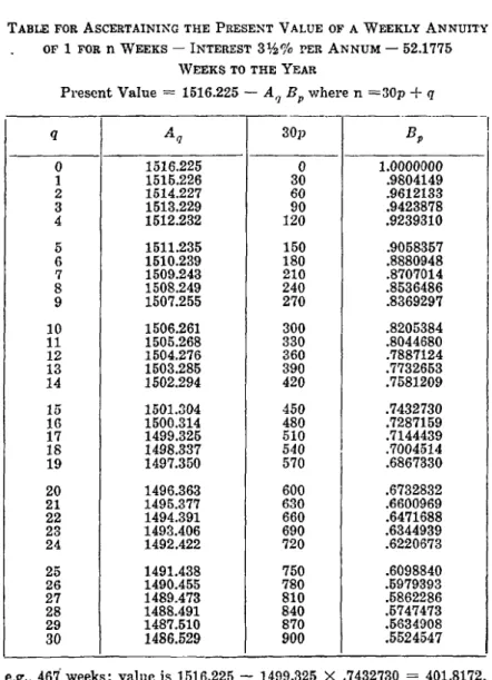
(8) T o construct a short table that will quickly give the present value of a weekly annuity for an), integral number of weeks not exceeding 900, assuming compound interest at the rate of 3~/2% per annum with 52.1775 weeks to the year. T h e value of a weekly annuity of 1 per week for n weeks is
D .(r) 1 -- v~- ruh-~ -- r
j ( r )
where r = 5 2 . 1 7 7 5 . Now if n = 3 0 p - ~ q we can write the value of the annuity as
I1 r r ?)r 30p X v7-
j~r~
A ,
2 . 30~r v T = A~ and v--~ - - Bp and construct tables of
I f we put j(r)
T A B L E S A D A P T E D F O R M A C H I N E C O M P U T A T I O N 143
required a n n u i t y value can be easily determined from the formula Ao - - Aq Bp. r 52.1775 First Ao --- .--- ~ - - 1516.2249405. .1¢o .034412769904 1 10 30 300 900
W e now calculate v r, v r , v ~, v r , v r from T a b l e s I, etc. T h e table of values of Aq we now get b y starting with Ao
1 1
and continually multiplying b y v ~, t h a t is A l - - v ~ A o ,
1 10 10
, 4 2 : v ~ A 1 , etc. We calculate A l o : A o v r, A e o - - A l o V *,
10 30
A3o ~ A2o v ~ - - ,4o v r , to be used as check values.
T h e tables of values of B r we get similarly b y continuous
30 30
multiplication b y v ~, thus Bo ~--- 1, B1 - - B o v r, etc. Check
300 300
values are obtained from Blo----v ~, B 2 o = B l o v r ,
300 900
B 3 o ~ B2ov r - - ' o r
T h e tables are calculated to 9 or 10 significant figures and later cut down to 7 figures. T h e completed tables follow:
1 4 4 TABLES ADAPTED FOR MACHINE COMPUTATION"
TABLE FOR ASCERTAINING THE PRESENT VALUE OF A WEEKLY ANNUITY oF 1 FOR n W E E K S -- INTEREST 3 ½ % FEE ANNUM - - 52.1775
WEEKS TO THE YEAR
P r e s e n t V a l u e ---- 1516.225 -- Aq Bp w h e r e n -~30p -P, q q Aq 30p Bp 10 11 12 13 14 15 16 17 18 19 20 21 22 23 24 25 26 27 28 29 30 1516.225 1515.226 1514.227 1513.229 1512.232 1 5 1 1 2 3 5 1510.239 1509.243 1508.249 1507.255 1506.261 1505.268 1504.276 1503.285 1502.294 1501.304 1500.314 1499.325 1498.337 1497.350 1496.363 1495.377 1494.391 1493.406 1492.422 1491.438 1490.455 1489.473 1488.491 1487.510 1486.529 0 30 60 90 120 150 180 210 240 270 300 330 360 390 420 450 480 510 540 570 600 630 660 690 720 750 780 810 840 870 900 1.0000000 ~ 8 0 4 1 4 9 .9612133 .9423878 .9239310 .9058357 .8880948 .8707014 .8536486 .8369297 .8205384 .8044680 .7887124 .7732653 .7581209 .7432730 .7287159 .7144439 .7004514 .6867330 .6732832 .6600969 .6471688 .6344939 .6220673 .6098840 .5979393 .5862286 .5747473 .5634908 .5524547 e.g., 4 6 7 " w e e k s : v a l u e is 1516.225 - - 1499.325 × .7432730 = 401.8172.
TABLES ADAPTED FOR M A C H I N E COMPUTATION 1 4 5
APPENDIX I
(1) It will sometimes happen that values of log (1-[-i) or jcr~ are required for a rate of interest not given in Tables I and II. In this case we can
either (a) calculate the value from Tables
III, IV,
v and VI. For log (1 + i) this calculation will be merely the determination of a logarithm e.g. for 3x'~e% we have to find log 1.033125 which can be readily done, but only to 10 place accuracy. For jcr~ we must calculate r { (1 + i)~--- 1) which involves finding the log (1 + i ) , and the antilogarithm of one r th of this. The final result will be accurate only to about 7 places, and the process is fairly long :or (b) we can interpolate in Table I or II as the case may be assuming (as will usually be the case) that the rate of interest for which the function is required is within the range of the Table. Now ordinary (first difference) interpolation is not sufficiently accurate neither is second difference interpolation. However, third difference interpolation is. The
8 h 4
maximum error is not greater than 1 ~ \ ~ ] where h is the interval between the values of ~ in the Table. For the first part of Table I (i.e. from 0% to 6%) k----.00125 and the maximum error is .00000 00000 0015 while from 6% to 10% h -- .0025 and the maximum error is .00000 00000 024 : as for Table I I k = .0025 and the maximum error is .00000 00000 017 for r~--2 rising to .00000 00000 055
f o r r - - oc.
The interpolation to third difference can be done by the usual central difference methods, but per- haps the easiest way is as follows : -
Use four tabulated values, two on each side of the value required. Then
(i) if, as will often be the case, the value is re- quired for i half way, quarter way or three quarters way between the tabulated rates,
~ 4 6 TABLES ADAPTED FOR MACHINE COMPUTATION
use the a p p r o p r i a t e one of the following formulas : - - --Uo + 9 Us + 9 u2 - - u3 ux~ - - 16 - - 7 Uo + 105 u~ + 35 u2 - - 5 u3 u l ~ " - 128 - - 5 Uo + 35 ul + 105 Uz - - 7 us or u ~ --- 128 (ii) T h u s if j~2) is required for 3 ~ % , Uo is jcz2~ for 2 ~ % , u~ t h a t for 3 % , u2 t h a t for 3~/~% and us t h a t for 31/~% : we require u l g which we get at once on the machine as 105 u~ plus 35 uz minus 5 u3 minus 7 Uo, the net divided b y 128. T h e answer is .030174165568. b u t if we require a value for a r a t e of interest, not half or q u a r t e r or three q u a r t e r s w a y between t a b u l a t e d rates, say log (1 + i) for 3.1%, proceed as follows :--choose Uo, u~, u2, us as before. L e t the required value be u l + , . I n t e r p o l a t e ( b y ordinary or first difference interpolation) between u~ and u2, t h a t is cal- culate x u2 + (1 - - x) u~ : call the result u'~+.~.
Do the same between Uo and u3 t h a t is cal- culate (1 + x) u3 + (2 - - x) Uo and call the
3 result u " l + ~.
T h e n the required Ul+~ is equal to u'l+~ + (1 - - x ) X ( u , + ~ _
2
U"l +~).
F o r instance in our example u o = l o g l . 0 2 8 7 5 , ul = log 1.03, u 2 = log 1.03125 and us = log 1.0325. W e require Ul.s. I n t e r p o l a t i n g for 3.1% between 3% and 3.125% we have
u'1.s = .8 u2 + .2 ul = .013258614187. Similarly interpolating between Uo and u~,
u " l . s = (1.8 u~ + 1.2 u o ) / 3 = .013257975485. N o w x (1 - - x ) / 2 = .08 and so
ul.s = u'l.s + .08 (u'l.s - - u"1.s) = .013258665283. • F r o m T a b l e s I I I , etc., we get the value of log 1.031
TABLES ADAPTED FOR MACHINE COMPUTATION 147 as .0132586652. T h e correct value is .013258665284. As another example let us calculate j~5-~) for 3.1%.
Uo - - j(5~) for 2 ~ % ul = j(~2) for 3% u2 - - j(m) for 31/~% us ---- jcw-) for 3~/~%. We require ul.4 u'1.4 - - .4 us -~ .6 ul - - .030537476446 . 1.4 ua ~ 1.6 uo __ .030531708137 u 1 . 4 - - 3 - - D i f f e r e n c e - - .000005768309 4 X .6 Multiply b y " 2 - - . 1 2 .000000692197 Add to
u'1.4
.030538168643 - - ul.4. T h e correct value is .030538168639 and the best we can get b y calculating from Tables I I I , IV, etc., is .030538144.Note:
When interpolating in Table I for i between 5 ~ % and 6~/~% we must remember that the inter- val for i changes at 6% and be careful to takeuo,
etc., at equal intervals, e.g. for 5.9% we must take Uo - - log (1 ~ i) for 51~%, ul for 53~%, u~ for 6% and ua for 6 ¼ % .
(2) If j(r) is required for a value of r not given in T a b l e II, e.g. ](G) we must either calculate from Tables I I I , etc., as indi- cated in (1) (a) above or else get the value b y summation of a series as for instance
jc~)--i
r - - 1 i2 + ( 2 r - - 1 ) ( r - - 1) is -2 r 6 r ~ . . . .
except that if )(,) is required for weekly annuities when the number of weeks to be assumed in a year is neither 52 or 52.1775 but some other near number, e.g. 52,~, we can inter- polate (or exterpolate if necessary) between j(52) and jcw..l~7.~). Thus f o r ] ' o , ~m put this equal to
(52.1775 - - 52~) )(~2) q- (52~ - - 52)
)f52.1775)
52.1775 - - 5297 j(~2) -{- 400
)(52,1775]
or jc52 1/n = 497148 T A B L E S ADAPTED FOR M A C H I N E C O M P U T A T I O N
Again if a year is assumed to equal 365¼ days we require j(~25/zs) : put this equal to (this is an exterpolation)
(52.1775 -- 5 2 ~ ) )(52) -1- (52-.~ - - 52) ](~2.1775> 52.1775 -- 52
--3 )(~2, q- 500 )(52.m5,
or j(55 5~2s~-- ' 4 9 7 "
For examplej(521/7) 3% will be found equal to .029567182004. API'ENDIX II
Examples (6) and (7) involve weekly annuities payable for so
many weeks and a ]faction o/a week. This brings up the question
of the interpretation of the results. What is meant for example by an annuity of 10 a week for 1061/~ weeks ?
The formula for a~ has been used above, and is usually used, as though it held for such non-integral periods. This evidently requires that if we have an annuity for an integral number of periods plus l t h of a period the value of the annuity payment
P
1
for the final I -lth of a period is 1 -- (1 q- " 3)-~, valued at the begin-
P Y
ning of such l t h period (that is just after the last full payment). P
In this formula ) is the effective rate of interest for a complete period. We now have two methods of making the final payment :-- (a) we can make it at the end of the l t h of the complete p e r i o d ,
P
when the amount of the payment should be 1
(1
+./),'
- - 1,
_ -1 which is slightly less than - .
P
(b) We can make it at the end of the next complete period, when
the amount of the payment should be
. 1 = - , ~ p l ) _ . . . )
(1 -1-- ]) - - (1 q- 3) -~- 1 / 1 +
J p
which is slightly more than 1 - - . P
T A B L E S A D A P T E D F O R M A C H I N E C O M P U T A T I O N 149 In practice, the amount of the final payment is invariably
1
taken a s - so that the total actual payments made correspond P
with the total period of the annuity. To conform to the above theory such a final payment of _1 should be made neither at the
P
end of the final complete period nor at the end of-lth of it but P
at a point approximately halfway between these two points. in practice the final payment, of ~, is usually made However,
A
at the end o f l t h of the period, except in the case of weekly P
annuities when it is often made at the end of the week. The theoretical error introduced by these sensible practical procedure is of course negligible.
APPENDIX III
So far in this paper and the examples it has been implicitly assumed that all the annuities dealt with are payable at the end of the period of payment; that is at the end of each year for yearly annuities, at the end of each week for weekly annuities and so on. The amounts and present values of annuities payable at the beginning of the period can be immediately derived from those of annuities payable at the end of the period as follows : -
Present value of an annuity of 1 per annum for n years payable (in installments of -1)- at the beginning of each -1th of a year equals
r r
a ~ _ ] % -1 r or alternatively a(r)/l~k _}_J'(r)~_~_]
Amount of an annuity of 1 per annum for n years payable (in installments of -1)- at the beginning of each l t h of a year equals
r r
~(r, 1 s~(l_t j(r,~
• - - or alternatively
1 5 0 TABLES ADAPTED FOR M~ACHINE CO~rPUTATION
AI'I'ENDIX IV
Up to this point it has been implicitly assumed that, in the case of an annuity payable r times a year, valued at rate of interest i, the rate of interest given is an
effective
annual rate and not anominal
annual rate convertible r times a year. If in any instances the given rate is a nominal one the valuation of the annuity is effected very readily by working in time units of lth of a year.r
For example the present value of an annuity of 1 a month for 60 months, at 3% per annum effective rate of interest is
1 ~ v 5
12 at 3%
j(12)
but at 3% per annum nominal rate convertible monthly it is 1 -- v e°
a t ¼ 9 .
Such calculations at nominal rates convertible with the same frequency as the annuity payments are relatively simpler than those at effective annual rates: the function j(r~ does not have to be used. The only difficulty that may arise is in the determination of log (1 + i) with sufficient accuracy. In the above example, 3 9 convertible monthly, the value of log (1 + i) for ¼ 9 is given in Table I, but if we required the value o f % 4 9 corresponding to 2 ½ 9 convertible monthly we must proceed as in Appendix I, that is either we would have to calculate log 1.002083333 from Table
III,
etc., or we must interpolate in Table I.In the case of weekly annuities, we are dealing with very low rates of interest (per week) : e.g. at 31/~9 convertible 52 times a
year the weekly rate of interest is ~ - - .000625 = ~ % and
unless we need extreme accuracy for a large number of weeks it will be sufficient to calculate log (1 + i) from Tables III, etc. If we do need greater accuracy than this gives, it is usually quicker to calculate log (1 + i) from the series
log (1 + i) ~ .4342944819 ( i - ~-2