The
NAS
Parallel
Benchmarks
2.1 Results
William Saphir *Alex Woo tand Maurice Yarrow [email protected]
Report NAS-96-010, August, 1996
Abstract
We present performance results for version 2.1 of the NAS Parallel Bench-marks (NPB) on the following architectures:
• IBM SP2/66 MHz
• SGI Power Challenge Array/90 MHz • Cray Research T3D
• Intel Paragon
"MILl, Inc. This work is supported through NASA Contract NAS 2-14303. tNASA Ames Research Center, Moffett Field, CA, 94035-1000.
tSterling Software, Palo Alto, CA. This work is supported through NASA Contract NAS 2-13210.
Contents
1 Introduction 4
2 Methodology 5
3 Applicability and usefulness of the results 3.1 Vector vs. Cache architectures ...
3.2 Mflop/s rates ...
3.3 Comparison with NPB 1 results ...
3.4 Comparing different configurations of the same type of com-puter ...
3.5 Relevance for other codes ...
6 6 7 7 Machines 9 4.1 NAS IBM SP2 ... 9
4.2 NAS SGI Power challenge array ... 10
4.3 Wright Laboratory Intel Paragon ... 11
4.4 JPL CRAY T3D ... 12
Code Descriptions 13 5.1 Application Benchmark: LU ... 13
5.2 Application Benchmark: SP and BT ... 14
5.3 Kernel Benchmark: MG ... 15 6 Results 6.1 6.2 6.3 6.4 6.5 6.6 6.7 15 Performance per processor ... 16
Total performance ... 18
Efficiency ... 19
Performance as a function of problem size ... 20
Differences in performance of different codes ... 21
Comparison of NPB 2 and NPB 1 performance ... 22
Discussion of clustered-SMP issues ... 24
7 Analysis/Conclusions 25
List
of Figures
1 Per-processor Performance ... 16MachineEfficiency ...
19
Performance
of threeclassesof LU on the T3D ...
20
Performance
of all ClassA codeson the SP2 ...
21
1
Introduction
The NAS Parallel Benchmarks (NPBs) [1, 2] are a widely-recognized suite of benchmarks originally designed to compare the performance of highly parallel computers with that of traditional supercomputers. The NPBs are specified algorithmically, and are implemented mainly by computer vendors, using techniques and optimizations appropriate to their specific computers. Performance results based on these optimized proprietary implementations are submitted to NAS by vendors and are reported in a periodic NAS Techni-cal Report [4]. The vendor-optimized NPB implementations will be referred to as NPB 1.
In late 1995, NAS announced NPB 2[3], a set of specific NPB implementa-tions, based on Fortran 77 and MPI[5]. NPB 2 implementations are intended to be run with little or no tuning, in contrast to NPB 1 implementations, which have been highly optimized by vendors for specific architectures. NPB 2 implementations are designed for computers with hierarchical cache-based memories.
Unlike that of proprietary NPB 1 implementations, the source of NPB 2 implementations is freely available. One advantage of this is that anyone can run them on any machine, allowing collection of data on a much wider variety of machines and configurations. Another is that the techniques used in NPB 2 implementations can be studied for possible use in other codes. Because they have not been optimized by vendors, NPB 2 implementations approximate the performance a typical user can expect for a portable paral-lel program on a distributed memory parallel computer. Together the results presented here provide a well-calibrated comparison of the real-world per-formance of several parallel computers. Furthermore, by comparing NPB 2 results to NPB 1 results, we can draw conclusions about how easy it is to obtain high performance on these systems. NPB 2 results complement, rather than replace, NPB 1 results.
NPB 2.1, upon which the results in this paper are based, was released in February, 1996. It contains implementations of 5 of 8 of the original NAS benchmarks - the three pseudo-applications LU, SP and BT, and the kernels MG and FT. NPB 2.2 will include the remaining benchmarks - CG, IS and EP - as well as a revised FT, which was found to have some scalability and
performanceproblems.This paperthereforeincludesresultsfor LU, SP,BT
andMG only. A future paperwill containresultsfor all 8 benchmarks.
This paper alsoincludesthe first resultsfor the NPB class"C" sizesthat
werefirst describedin the NPB 2.0report.
2
Methodology
NPB 2 presents a number of challenges and opportunities that were not present in NPB 1. NPB 1 implementations represent a best case scenario: they are implemented and carefully optimized by vendors (and the codes remain proprietary); they are run by vendors in ideal conditions in clean en-vironments with the latest software. NPB 1 results are meaningful and can be compared because every vendor has had equal opportunity to optimize, and because the pencil-and-paper nature of the benchmarks eliminates ar-chitectural bias. NPB 1 results, while far more meaningful than the "not to be exceeded" peak performance and LINPACK[6] rates, generally represent upper limits on what can be achieved for the type of calculations performed by the NPBs.
In contrast, NPB 2 implementations are run essentially "out of the box" with no tuning 1. Because the NPB 2 codes are not proprietary, and source is readily available and easy to build, anyone can generate NPB 2 results. The environment in which the benchmarks are run may not include the latest software and hardware, may not include all the special tuning tricks known to vendors, and may not be as clean as that used by vendors. As with any scientific measurement, benchmark results are useless unless reproducible. Therefore great care must be taken to document the specific conditions under which measurements were made - compiler options, MPI and compiler versions, system software version, etc.
In this report, section 6 describes the environment in which the measure-ments were taken. The conditions were the best available to NAS when the measurements were made. While the environment description may make the results more difficult to understand (especially when there are several sets of results for the same "machine" with slightly different configurations),
1NPB 2 permits two levels of tuning: 0% code modification and 5% code modification. This report contains results only for the 0% case
data qualifiedin this waycanprovidea well-calibratedmeasurement
of the
effectof smallhardwareand softwarechanges- showingthe improvement
or regressionof systemperformanceovertime.
All NPB 2 implementationsdiscussed
in this paperrun a
singlesolveriter-ation and resetthe initial conditionsbeforestarting the the timed portion
of the benchmark. This procedureeliminatesstartup time overheadthat
canseverelyskewresultsfor short-runningbenchmarks.It alsomeansthat
Mflop/s rates reportedby the codewill not be the sameas Mflop/s rates
reportedby a hardwareinstructioncounter.Caremustbe takento
recon-ciledirectly-measured
operationcountswith the ratesreportedby the codes
themselves.The measurements
canbereconciledby directly measuringthe
operationcountof zero-iterationrun andsubtractingthis from the
opera-tion count of a completerun. The time reportedby the benchmarksand
in this report is wallclocktime. CPU time haslittle meaningin a
tightly-coupledparallel programwheretime spentblockingfor messages
may not
be countedasCPU time.
3
Applicability
and
usefulness
of the
results
3.1 Vector vs. Cache architectures
In this paper we report results only for machines based on RISC proces-sors with cache-based memory hierarchies. While Fortran and MPI provide compile-and-run portability, it is much more difficult to obtain architectural portability, that is, to design a code that can run efficiently on both vector and RISC/cache architectures. In many cases, the requirements for a vector code (long vector length) directly conflict with those for a cache code (cache reuse). In some cases, it is possible to write a code that runs well on both, particularly when vendor-optimized libraries can be used. The NPBs do not use such libraries.
NPB 2 implementations are written specifically for cache-based architec-tures, and assume a fully distributed memory model, with communication only through MPI. While the codes can be run on a vector machine, such as a Cray J90, the results cannot be meaningfully compared with other re-suits, except to point out the fact that compile-and-run portability does not
In this report wecompareresultsfrom four machines.Threeof these
- the IBM SP2, Cray T3D, and Intel Paragon with GP nodes - have completely distributed memory. One - the SGI Power Challenge Array - is composed of SMP nodes.A few types of machines, including traditional networks of workstations, are not represented here but will be included in future reports.
3.2 Mflop/s rates
A new feature of NPB 2 is that we report results in Mflop/s (million floating point operations per second) as well as run time. The Mflop/s measure has little meaning for NPB 1, since different implementations may have substantially different operation counts. Since NPB 2 results are based on unmodified code (0% case), the operation count is approximately the same on any machine. Good optimizing compilers may be able to eliminate some operations, and others may add operations for certain reasons, so the reported Mfiop/s rate may not be exactly what would be reported by a hardware instruction counter, but in our experience it is usually quite close (within a few percent).
The nominal rate is based on a combination of hand counting, hardware instruction counting (originally on Cray machines, more recently verified on an SP2) and extrapolation. The nominal floating point count does not change with number of processors - only with problem size - so any extra operations performed because of parallelization are not counted.
3.3 Comparison with NPB 1 results
In all cases, we compare NPB 2 results with NPB 1 results for the "same" machine. While this comparison is interesting, we do not want to overstate its significance. Roughly, the comparison shows the difference between what an "ordinary programmer" can achieve on a portable program and what an expert or unusually careful non-expert can achieve on an architecture-optimized program. If NPB 1 and NPB 2 timings are quite close, one might conclude that it is relatively easy to get "peak" (where peak means NPB-1 level) performance out of a particular machine. Different machines have substantially different results for this metric.
3.4 Comparing different configurations of the same type of computer
While the NPB suite was originally designed to compare different types of computers, it can also be used to probe certain minor differences within a single type of computer. For instance, the effect of using different compiler flags, different versions of the MPI library, and even different compilers (e.g.,
Fortran 90 vs. Fortran 77) can be measured. In this report, we use the NPB suite to explore different configurations of an SGI Power Challenge cluster, where a given number of processes may be distributed across nodes in many different ways.
3.5 Relevance for other codes
The NPB suite is based on computational fluid dynamics (CFD) codes typi-cal of those run on the supercomputers at the NAS facility. We believe that
the NPB 2 results are relevant to "the average user, with an average code," with a few caveats.
First, the NPB 2 implementations do not use numerical libraries. Codes that use vendor-optimized numerical libraries may obtain substantially bet-ter performance. Some library routines that could be useful for NPB imple-mentations are FFT routines for the FT benchmark, a pentadiagonal solver for the SP benchmark and a block-tridiagonal solver for the BT benchmark.
NPB 2 implementations do not use these because there do not exist stan-dardized, vendor-optimized and widely available versions of the necessary routines (unlike the BLAS routines, which are less useful for the NPB prob-lems).
Second, most NPB codes use fully implicit algorithms on a single grid that is distributed over several processors. Such algorithms require more com-munication than explicit methods or hybrid methods that solve implicitly on a single processor with explicit updates between processors. Compared to codes using these other algorithms, the NPB suite provides a more strin-gent test of interprocessor communication, and may show poorer scalability. Counteracting this is the fact that the NPB 2 codes use good parallel algo-rithms that minimize communication.
are moreregularthan typical real-worldproblems(makingload balancing
easier)andboundaryconditionsandphysicshavebeensomewhatsimplified.
The effectson performanceare complicated.For instance,load-imbalance
from boundarycalculationsis probablysmallerthan in engineering
applica-tions, but havingfeweroperationsper grid point per time step (becauseof
simplerphysics)givesa highercommunicationto computationratio.
For thesereasonsandothers,performanceof real-worldcodesmay or may
not be similar to NPB performance.The main useof NPB is, instead,to
comparetheperformance
of differentcomputersonthe generalclassof codes
representedby the NPBs.
4
Machines
The results presented in this report were collected on an IBM SP2, an Intel Paragon, an SGI Power Challenge Array, and a Cray T3D.
4.1 NAS IBM SP2
IBM SP2 results were collected on the machine located at the Numerical Aerodynamic Simulation (NAS) facility at NASA Ames Research Center. This SP2 contains 160 "wide" nodes, each with a single POWER-2 processor running at at 66.5 MHz, and with a theoretical peak performance of 266 Mflop/s. The nodes are connected by a high performance switch. All nodes have at least 128 MB of main memory.
The key feature of wide nodes, for the purposes of this report, is that they have (when configured with the right number of memory cards) a very wide (256 bit) path between the processor and main memory that provides ex-traordinary memory bandwidth (about 2 GByte/s per processor). They also have a 256 KB primary cache with 256-byte cache lines. These figures are twice and four times what is available on the so-called "thin-node 2" and
"thin-node", respectively.
IBM has implemented an optimized version of MPI for the SP2. The point-to-point bandwidth of this MPI is about 35 MB/s. The latency is about 55
#S.
• AIX version 4.1.3
• POE version 2.1 (includes MPI) • XL Fortran version 3.2
The following compiler flags were used in compiling all NPB 2 codes (all but the last are defaults on the NAS system, but not on all SP2 systems):
• -qcache = typ e= d:level= 1:size= 256,-qarch= pw r2 - O 3
The nodes of the NAS SP2 are always dedicated to a single user process. Many of the results were collected when other jobs were running on the system. The only effect these jobs would have would be on placement of processes and switch contention. Neither of these has had a noticeable effect on system performance for the number of nodes on which we collected results. All codes were run three times. The best times were chosen for this report. IBM provides a "high priority" mode to run applications. This is not turned on by default on the NAS machines, and we did not use it. It allows the effect of competing system processes to be minimized.
4.2 NAS SGI Power challenge array
The SGI Power Challenge Array located at NAS is a cluster containing 4 Power Challenge SMP nodes, each with 8 R8000 processors running at 90 MHz. (The NAS system includes a few other nodes, but they were not used for this report). Each processor has a peak floating point performance of 360 Mflop/s. For a few of the measurements, we moved 18 processors into a single node and ran code on that single node. See section 6 for more details. Each of the 4 nodes has two HIPPI connections. All HIPPI connections are switched on a single switch.
SGI has implemented an optimized MPI for the Power Challenge Array. Within a single node, MPI transfers are done through a single-copy mech-anism, achieving 64 MB/s bandwidth and 18 #s latency. Between nodes, transfers are done with a special HIPPI driver that bypasses (but coexists with) IP traffic. MPI transfers over HIPPI achieve about 110 tts latency and 92 MB/s bandwidth. Very large data transfers are striped across multiple HIPPI connections, giving about 160 MB/s over 2 HIPPI connections. None of the NPB 2 implementations discussed in this paper sends messages large
enoughto makeuseof this feature,however.The FT benchmark,whichis
currentlyundergoingrevision,will makeuseof it.
The _llowing so,warewasused_rthe resultspresentedin this paper:
IRIX version 6.12
MPI version 2.0
MIPSpro Fortran version 6.2
The compiler flag"-03" was used _r allcompilations.
The nodes of the NAS cluster are always devoted to a single user job, so there is no contention for memory bandwidth with other jobs. In an SMP-based cluster, there is considerable freedom in how to arrange processors among nodes. Some of the competing considerations (for a fixed number of processors to be distributed over some number of SMP nodes) are:
.
.
,
Increasing the number of processors in a node to make use of low-latency communication within a node
Decreasing the number of processors in a node to reduce the effect of memory contention.
Using at least 1 fewer processes than processors on a node to avoid competition with system processes.
We have done some experimentation with different configurations. Unless otherwise noted, most reported results are the best obtained with several configurations. In section 6 we discuss the effects above in some detail. 4.3 Wright Laboratory Intel Paragon
Intel Paragon results were collected on the Intel Paragon located at the ASC Major Shared Resource Center (MSRC) X/PS-25 at USAF Wright Laboratories. It contains 368 compute nodes, 9 service nodes, and 24 multi-purpose I/O nodes. 352 of the compute nodes have 32 MB of memory, while 16 have 64 MB of memory. The machine has a 24-disk RAID system attached as a Parallel File System work area, with a total available space of 22 GBytes. All results were obtained from the General Purpose (GP) nodes. Each GP node has two i860/XP RISC processors: one processor is used for computation, the other for communication under OSF UNIX. Theoretical
peak performance of the i860/XP GP node is 75 Mflop/s (double precision).
(The Multi-Purpose (MP) nodes have three i860's and two can be used for
computation under OSF UNIX.)
The nodes are connected by a network with the topology of a two-dimensional
mesh. Messages are packetized and routed using dimension-order routing.
Messages are automatically routed through intervening nodes without
inter-rupting the processor. The network has a latency of 66 #s and a bandwidth
of 70 MB/s for MPI messages.
The following software was used for the results presented in this paper:
0SF/I Release 1.0.4 Server 1.4 RI_4 with Patch RI.4.1
MPI Vl.0.12 external version - compiled with ch_nx lib
PG FORTRAN I%5.0 Patch R5.0.3
The following compiler flags were used in compiling allof the NPB 2 codes:
-04 -Knoieee
All runs were made under the Network Queuing System (NQS) where each
node was dedicated to a single job with the -plk page lock fag. The only
effectother batch jobs would have would be on the physical placement of
processors and network contention.
4.4 JPL CRAY T3D
The CRAY T3D results were collected on the CRAY T3D SC256/264 at
the JPL/ESS Parallel Computing Testbed. This T3D contains 256 DEC
21064 (Alpha EV4) processors. Each processor has a peak performance of
150 Mflop/s. The combined theoretical peak speed is 38.4 Gflop/s. Each
processor has 64 MB of memory. Each processing element (PE) in the
CRAY T3D system comprises the DEC Alpha microprocessor, local memory,
and support logic. The PE is the basic computational unit in the CRAY
T3D system's multiple instruction multiple data (MIMD) architecture. A
CRAY T3D system node consists of two PEs sharing the switch and network
support logic.
The PEs are connected by a bidirectional 3-D toroidal network. The
hard-ware peak interprocessor communication rates are 300 MB/s in every
di-rection through the torus, resulting in a bisection bandwidth of up to 76.8
GB/s.
The version of MPI supplied by CRAY originated from the Edinburgh Par-allel Computing Centre version 1.5a with extensions. Its latency is about 37 #s, and its bandwidth is about 28 MB/s.
The following software was used for the results presented in this paper:
UNICOS 8.0 Cray CF77_M Version 6.0.4.3 Cray GPP_M Version 6.0.4.2 Cray CFT77_M Version 6.2.1.4 (6.62) (6.17) (281382)
The following compiler flags were used for all NPB 2.1 codes:
-dp -Wf-oaggress -Wf-onoieeedivide -C cray-t3d
and the following load options:
-Wl-Drdahead=on -C cray-t3d
All results were obtained either interactively or with NQS batch jobs. The nodes were dedicated to the benchmark run but there was a possibility of network contention with processes on other nodes.
5
Code
Descriptions
5.1 Application Benchmark: LU
The LU benchmark solves a finite difference discretization of the 3-D com-pressible Navier-Stokes equations through a block-lower-triangular block-upper-triangular approximate factorization of the original difference scheme. The LU factored form is cast as a relaxation, and is solved by SSOR. The LU benchmark is based on the NAS NX reference implementation from 1991, but communication in the SSOR procedure has been considerably simplified. The NPB 2 LU code requires a power-of-two number of processors. A 2-D partitioning of the grid onto processors is obtained by halving the grid repeatedly in the first two dimensions, alternating between x and y, until all processors are assigned, resulting in vertical pencil-like grid partitions. Each pencil can be thought of as a stack of horizontal tiles. The SSOR procedure is implemented as a generalized pipeline. Starting with the bottommost tile of a corner pencil, pointwise SSOR operations proceed along lines of the tile
in the unit-stride direction, until all points on the tile havebeenrelaxed.
Neighboringtiles are sent updatedvaluesalongadjacentedges,and these
pencilscannow processtheir respectivetiles, whilethe first processorcan
now processpointson the next tile above. Processingthus proceedson a
"hyperplane"of activetiles. The pipelinespendsrelativelylittle time filling
andemptyingandis perfectlyload-balanced.
Communicationrequirements
aresmallcomparedto computationexpense,
makingthis parallelLU scheme
relativelyefficient.
Cache line reuse in the relaxation sections is high.5.2 Application Benchmark: SP and BT
Like LU, SP and BT use an implicit algorithm to compute a finite-difference
solution to the 3-D compressible Navier-Stokes equations.
The solution is based on a Beam-Warming approximate factorization. The approximate factorization decouples the x, y and z dimensions, resulting in three sets of narrow-banded, regularly structured systems of linear equations
that can be solved directly.
In SP, the flux Jacobians are fully diagonalized, and the resulting systems are scalar pentadiagonal (reflecting the presence of fourth order artificial dissipation) In BT, the resulting equations are block-tridiagonal (the fourth order dissipation appears only on the right hand side, so the left hand side difference stencil has a width of only 3), with (5 × 5) blocks. In both cases, the systems are solved using the Thomas algorithm - Gaussian elimination (GE), without pivoting, of a banded system. Parallelism in the solution phase appears both in the data (solutions along parallel grid lines can be computed independently, since they have been decoupled by approximate factorization) and through GE pipelining.
To solve these equations, both SP and BT use the multipartition [7] method. Each processor is assigned several non-overlapping sub-blocks (partitions) of points. This domain decomposition provides near-perfect load balance, re-quires only few data movements of moderate size along partition boundaries,
and has no pipeline fill delay. Tradeoffs between this and other methods are described in [8].
Both SP and BT have two phases in each iteration. The first phase is the computation of the right hand side, which is identical in the two codes. It
involvescompactlocal differencestencilsonly. The matrix solutionphases
proceedasdescribedabove.Thecoreofthe SPsolutionphaseis thesolution
of pentadiagonal
systemsusingGE.Thereis verylittle datareuse.The core
of the BT solutionphaseinvolvessolutionof (5x 5)-systems
ofequationsand
multiplicationof (5 × 5) matrices,both of whichaxepart of the application
of GE to the block-tridiagonalsystems.Thereis significantlymore data
reusein theseoperations.
Both the SPandBT codesrequirea squarenumber
of processors because of the decomposition requirements of the 3-D multipaxtition method. These codes have been written so that if a given parallel platform only permitsa power-of-two number of processors to be assigned to a job, then un-needed processors are made inactive, but are counted when determining Mflop/s/process rates.
5.3 Kernel Benchmark: MG
The MG benchmark implements a V-cycle multigrid algorithm to solve the scalar discrete Poisson equation. This benchmark code is based on the 1991 reference implementation written by NAS. Four critical subroutines - the smoother, the residual calculation, the residual projection, and the trilineax interpolation of the correction - were optimized for both vector and RISC processors. These routines represent the vast majority of the total work. There are two different explicit smoothers used derived from trilinear finite elements. Most of these routines work well because they use continguous stride one memory access or, in the case of the smallest grids, the entire array fits in cache. This code requires a power-of-two number of processors. The partitioning of the grid onto processors occurs such that the grid is successively halved, starting with the z dimension, then the y dimension
and then the x dimension, and repeating until all processors are assigned. The MG benchmark pushes residuals and pulls solutions from dense to coarser grids and thus has short messages of different lengths based on the grid sizes.
6
Results
NPB 2 data can be used to examine a number of performance issues. In this report, we highlight a few of the more interesting results, using a single
resentative sample from a large number that could have been used. Detailed
, graphs of all NPB 2 results are available at http://www.nas.nasa.gov/NAS/NPB/NPB2Results/.
6.1 Performance per processor
03 O_ 0 R r_ o 7O 60 50 4O 3O 2O 10 o
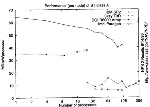
Performance (per node) of BT class A
... IBM SP2
'---_---Cray T3D ----_....
SGt R8000 Array .... _,.... _,-._._._._. Intel Paragon ...e...
... t[ ... t1""'" D ¸ • - • 6 ¸¸ ..-_1 ... D.-D I I I I I I I 2 4 8 16 32 64 128 256 Number of processors 0_
z
¢oo0 o_<_z
,,--> _o _¢:?. q) o_ n-oi cu_ Z :=::t-Figure h Per-processor Performance
Figure 1 shows the per-processor performance of BT class A on all
ma-chines. It shows a large disparity in per-processor performance between
the four machines. The SP2 is the clear leader, obtaining as many as 65
Mflop/s/processor (but as few as 40 Mflop/s/processor on 100 nodes)• The
Power Challenge Array is a distant second with about 35 Mflop/s/processor.
The T3D is substantially below that at about 10 Mflop/s/processor, and
the Paragon registers barely more than 5 Mflop/s/processor. This ranking
is consistent across all benchmarks•
The maximum Mflop/s/processor values obtained on each machine are:
SP2 :
PC Array :
85 Mflop/s/process on NG class B i processor
46 Mflop/s/process on NG class B I processor
Paragon:
T3D:
8 Mflop/s/process
on MG class B 64 processors24 Mflop/s/process on LU class C 128 processors
We do not have at this point an explanation for why all machines except
the T3D prefer MG.
The actual performance is not proportional to peak performance, which is:
SP2: PC Array: Paragon: T3D: 266 Mflop/s/processor (66.5 MHz) 360 Mflop/s/processor (90 MHz) 75 Mflop/s/processor (50 NHz) 150 Mflop/s/processor (150 NHz)
We attribute the dominance of the SP2 to its high memory bandwidth. The
other machines have far poorer memory bandwidth relative to peak
perfor-mance. The SGI partially makes up for its poor memory bandwidth with
its very large (4MB) secondary cache. We note that as of this writing, none
of the above processors is state-of-the-art. The i860 is no longer produced,
the Alpha 21064 in the T3D has been replaced by a a faster chip, the R8000
in the SGI Array will soon be superceded by the R10000, and the Power 2
multi-chip processor is now available with a higher clock rate.
We also note that performance of the SP2 falls off rapidly with number
of processors. This is because its inter-node communication performance
is relatively poor compared to its floating point performance. Fairly level
lines for the Paragon and T3D out to 128 and 256 processors indicate good
relative network performance. For the SGI Array, the maximum number of
processors used was 32 spread over 4 nodes, so it was not possible to test
scaling properties as much as on the other machines.
The sawtooth appearance of the T3D line results from the fact that a T3D
may allocate only a power-of-two number of nodes. Thus, is is necessary to
use 256 nodes when a problem requires only 144. The NPB 2 codes calculate
per-processor performance on the basis of total allocated, not total used.
6.2 Total performance O m 10000 1000 I O0 I0
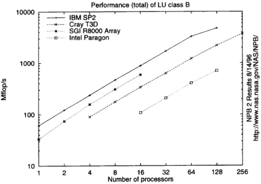
Performance (total) of LU class B
' IBM S1_2 ... ----_ .... Cray T3D .... _,.... SGI R8000 Array ..._ ... Intel Paragon _ ..--"" ,._C.////'''x/" f" I I I I I ,I I 2 4 8 16 32 64 128 256 Number of processors O. z _C n-o_ z =:;
¢-Figure 2: Total Machine Performance
Figure 2 shows total machine performance for LU class B. The information content is similar to that in Figure 1, except that it is easier to judge total machine performance. Among the machines we tested, the NAS SP2 still has the highest performance, even though it does not have as many nodes as the T3D or Paragon that were tested.
6.3
Efficiency
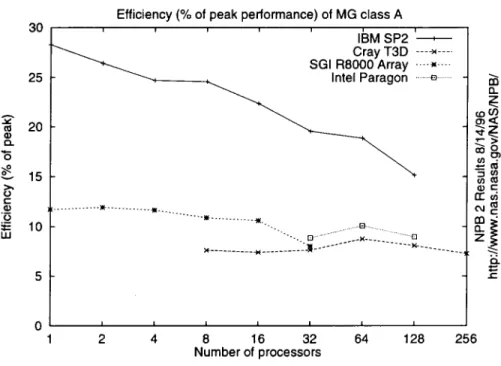
3O 25 o_ 20 (D ¢:1,. "6 e.-_ 10 u.iEfficiency (% of peak performance) of MG class A
' ' ' IBM SP2 '-_ Cray T3D ----x .... SGI R8000 Array .... _,.... Intel Paragon ..._ ... "-. ...E) ... ""-.. [3 ... ..-X ... ...E] I I I I I I I 2 4 8 16 32 64 128 256 Number of processors 12. rc_ oJ_ z H
¢.-Figure 3: Machine Efficiency
Figure 3 shows the machine efficiency on MG class A. Efficiency is total Mflop/s divided by the peak Mflop/s, expressed as a percentage. The most interesting point of this graph is that it shows that the SP2 obtains its high performance not through high peak performance, but by attaining a rela-tively large fraction of peak performance - as much as 24of peak performance. This result emphasizes the inappropriateness of relying on peak performance to judge the capabilities of RISC-based machines. Though they are not rep-resented here, vector machines typically attain a much higher percentage of peak performance on appropriate, well-written codes.
6.4
Performance
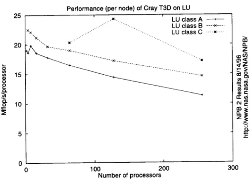
as a function of problem size 25 20 (D 15 0 2 o 10Performance (per node) of Cray T3D on LU
i i .-_=._. LU c ass A ... LU class B ----_ .... Ix× ... LU class C .... _ .... ... x-. '.. "--_-->( .... "N( I I 0 1O0 200 300 Number of processors (3. z
t-Figure 4: Performance of three classes of LU on the T3D
Figure 4 shows the performance of LU class A, B and C on the T3D. The largest size, class C, clearly performs the best on any given number of proces-sors. We attribute this largely to the fact that the computation to commu-nication ratio is highest, due to the best surface-to-volume ratio. A detailed analysis shows that this is not the only factor at work, as it does not exactly predict performance.
6.5
Differences
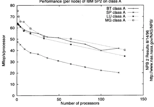
in performance of different codes 8O 7O 6O 5O (l) fJ Q. 40 0 _- 30 2O 10 0Performance (per node) of IBM SP2 on class A
i i BT class A --SP class A ... LU class A .... },.... _}o MG classA • e .... '.. ". ''B. - '''"_---. ... E3 ... ,( "'".--.... ... "X ... -}i.... ... ""O I I CO O. Z rr_ z e-" 0 50 100 150 Number of processors
Figure 5: Performance of all Class A codes on the SP2
Not all NPB codes perform equally well. For instance, Figure 5 shows the performance of all class A codes on the SP2. MG, LU and BT have approx-imately the same performance, in Mflop/s, but SP exhibits substantially lower performance in Mflop/s/processor.
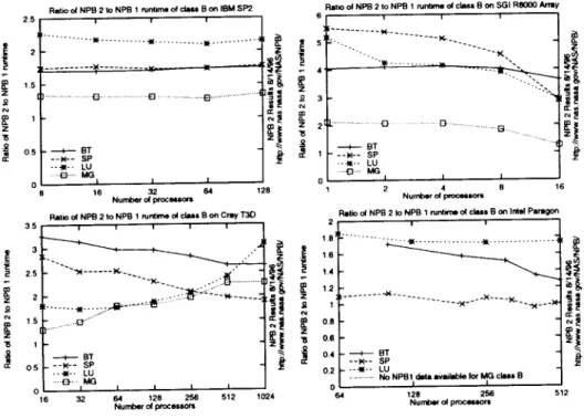
6.6 Comparison of NPB 2 and NPB 1 performance
It can be insightful to compare NPB 2 and NPB 1 results. While NPB 2 results can be reported in Mflop/s/processor, NPB 1 implementations may have different operation counts. Instead of Mflop/s/processor, we plot a the ratio of NPB 2 run time to the NPB 1 run time.
Because NPB 1 and NPB 2 data are not always available on the same num-bers of processors, we calculate a ratio based on a fit of Amdahl's law to the NPB 2 results. 2.5 2 : Z_ 1,5 2 I ]5 05
:ratio of NPB 2 to NPB 1 runtirng of = B on IBM SP2
6 ; i i _ - [¢ ...El...E] ...E}..._] 3 _ BT
| ,
-- -_-- LU p_m Bm_ MGI I I 0 B 16 32 64 128 183 z]5 o.,
N _ 0.4 :_ 0.2 o Number o_ processorsRatio o_NPB 2 to NPB 1 runtlme o4cl_s B on Cray "1"30
3sI ... 2: ..._...:.._B... e:::::__::'_:':-'*-1 5 . .._"'" .... I , BT 05 ---)<-- SP --_-- LU ....•El--,MG I I I i I 016 32 64 128 256 512 1024 Numberof processors
Rat0o od NPB 2 to NPB 1 rur,_no o_clau B oft SGI RSOOO Am
J i i E.. ... )¢._. ... {:3 ... O...{3 BT - -)<-- SP --_-- LU ....O'- MG I I I 2 4 B 16 Numberof ptocee.lonl
Rlltio of NPB 2 Io NPB 1 run_e of class B on Illel Psrlgon
2 ! i
... -4(-___ ... ____X. -->( --)(- _.._.__)q
BT
- -)<-- SP
_ --_-- LU
I ... No NPBI data ivlilad>le f_ MG clsuB
[ I I
128 256
Nurni0_ o_ pmc_m_m
512
z!
Figure 6: Ratio of NPB 2 to NPB 1 run time
Figure 6 shows the NPB 2 to NPB 1 run time ratio for all benchmarks on
each machine. Higher numbers mean that NPB 1 performs better relative to NPB 2. Positive slopes show NPB 1 scaling better, and negative slopes show NPB 2 scaling better. Taking NPB 1 performance as the "peak achievable" performance, and NPB 2 performance as "normal" performance without a lot or architecture-specific tuning, we can make a statement about how much architecture-specific tuning is necessary to obtain high performance on each
machine.
The Paragonhasthe smallestratios betweenNPB 2 and NPB 1
perfor-mance. For the SP2 the ratio is usuallybetween1 and 2. For the T3D,
NPB 2 performsrelativelyworse,between1.5and3 timesslower.The SGI
Array resultsshowthe worstrelativeperformanceon NPB 2.
Takingthis informationtogetherwith theper-processor
performance
results,
weconcludethe following.The SP2designmakesit relativelyeasyto obtain
a high percentageof peakperformance.On the T3D and SGI it is much
harderto achievegoodperformance,
but carefularchitecture-specific
tuning
can improvethe situation considerably.Architecture-specific
tuning may
buy youmoreonthe SGIthan onthe T3D. Finally,the Paragoni860nodes
arerelativelyinsensitiveto tuning.
6.7
Discussion of clustered-SMP issuesThe architecture of the SGI Power Challenge Array is quite different from the other machines that were tested, in that it is based on SMP nodes, rather than single processor nodes. In this respect, it is similar to many currently planned products from other companies.
In the earlier days of parallel computing, network topology could be quite important. For instance, communication patterns on a hypercube-based computer such as the Intel iPSC/860 had to take into account the topology of the network. On later machines, such as the SP2, the T3D and the Paragon, network topology effects still exist, but are usually much less important. They can often be considered "topology free", especially when there is an intelligent scheduler.
The Power Challenge Array may represent the first in a new generation of parallel computers and a return to the days when it mattered where pro-cesses were placed. There is non-uniformity both in the "network" (shared-memory communication has lower latency, lower point-to-point bandwidth, and higher aggregate bandwidth than inter-node communication) and the processors (two processes on the same SMP node may share a memory bus, competing for memory bandwidth, or may be on different nodes, with no competition for bandwidth). These two factors affect the configuration (op-timal number of processors per node) and placement of processes on a set of nodes.
We note that a solely message-passing based code may not be the most efficient type of code on an SMP-based cluster. Indeed, it may be beneficial to use compiler-exploited parallelism within a node and MPI between nodes. While this may turn out to be an efficient model, it is not yet clear that it will be generally useful. For instance, compiler directives are not portable, and requiring the programmer to find two different types of parallelism may be unrealistic. There may be other reasons why such a program designed
for such a system may not run well on a fully distributed system.
We obtained Array results for as many different configurations as were fea-sible. For instance, 16-process results were obtained for 16 processes on a single node, 8 processes on each of 2 nodes, and 4 processes on each of 4 nodes. The resulting data reflect a competition between reduced memory
contentionwhenspreadingprocesses
amongnodesandreducedcommuni-cationperformancebetweennodes.
Someof the resultsof this experimentare summarizedin table one. It
is immediatelyevidentthat memorycontentionbecomesan issueevenat
very small numbersof processors.For instance,onecan usually obtain
substantiallybetterperformance
for an 16-process
job by placing8 processes
on eachof 2 nodesthan by placingall 16processes
on a single16-processor
node.2
Table1: Table1. Mflop/s/processfor differentconfigurations
bt.A
bt.B
lu.A lu.B
mg.A mg.B sp.A sp.B
16procsx 1 node 18.5 13.8 39.7 29.0
17.8
19.2 27.7 14.2
8 procsx 2 nodes 32.1 26.9 33.9 34.1
29.6
31.9 35.6 26.5
4 procsx 4 nodes 36.2 31.2 37.8 36.7
38.2
39.9 37.4 N/A
7
Analysis/Conclusions
In this paper we have presented what we consider baseline NPB 2 results. All machines for which we have reported results have been or will soon be displaced by faster successors. We intend to track the performance of newer machines and report their performance in the same manner. It will also be interesting to see how much performance increase can be obtained at the 5% modification level allowed by the NPB 2 rules. It remains to be seen whether small changes to these portable codes can significantly increase performance. Vendors and others are encouraged to submit results.
The results shown here confirm several facts that are well known in the high-performance computing community: that actual performance on RISC processors is often around 10% of peak performance; that SP2 processors perform best and Paragon i860 processors (which are much older) perform worst; that careful architecture-specific tuning can improve performance sig-nificantly; that the SP2 has a relatively underpowered network.
2Note: 16 process cases run on 18-processor node 2x8 process cases run on 2 8-processor nodes 4x4 process cases run on 4 4-processor nodes
Wehavealsoshownthat the NPB 2 suitecanbe usedto
makecarefulmea-surementsof a singlemachine.In additionto the SMPclusterconfiguration
analysisdiscussedin section6, NAS hasbeenusing the NPB 2 suite for
regressiontestsand the analysisof the effectof newsystemsoftwareon
applicationperformance.
By the end of 1996,we expectto releasea completeset of NPB codes
(including IS, CG, EP and a rewritten FT) as well as resultsfor those
codes.
Acknowledgment
The NAS parallel systems group was extremely helpful in many stages of collecting the NPB 2 results. Lou, Archie, James and Mary often went out of their way and beyond the call of duty to help out when there were problems or special requests. Memories of specific instances have faded, but to take a recent example, the other week Lou swapped a bunch of boards in davinci so that we could obtain the 16-processor 1-node results.
We would also like to thank Barbara Horner-Miller for providing access to the JPL CRI T3D machine and allowing us to greatly exceed our CPU quota.
We would also like to thank Kueichien Hill and Robert Pollick for allow-ing us the use of the Wright Laboratory Paragon.
References
[1] Bailey, D. H.; Barszcz, E.; Barton, J. T.; Browning, D. S.; Carter, R. L.; Dagum, L.; Fatoohi, R. A.; Frederickson, P. O.; Lasinski, T. A.; Schreiber, R. S.; Simon, H. D.; Venkatakrishnam, V.; and Weeratunga, S. K.: The NAS Parallel Benchmarks, International Journal of
Super-computer Applications, Vol. 5, No. 3, (Fall 1991), pp. 63-73.
[2] Bailey, D. H.; Barton, J.T.; Lasinski, T. A.; and Simon, H. D., eds: "The NAS Parallel Benchmarks," NASA Technical Memorandum
103863, NASA Ames Research Center, Moffett Field, CA, 94035-1000,
July 1993 http://www.nas.nasa.gov/NAS/NPB/.
[3] Bailey, D. H.; Harris, T.; Saphir, W.; van der Wijngaaxt, R.; Woo, A.; and Yarrow, M., "The NAS Parallel Benchmarks 2.0,"NASA Technical
Report NAS-95-020, NASA Ames Research Center, Moffett Field, CA,
94035-1000, December 1995 http://www.nas.nasa.gov/NAS/NPB/.
[4] Bailey, D. H.; and Saini, S., "The NAS Parallel Benchmarks Results 12-95,"NASA Technical Report NAS-95-021, NASA Ames Research Center, Moffett Field, CA, 94035-1000, December 1995 http: / /www.nas.nasa.gov /NAS /NPB /.
[5] Message Passing Interface Forum: MPI: A Message---Passing Interface
Standard, Version 1.1, July, 1995, http://www.mcs.anl.gov/mpi/mpi-report- 1.1/mpi-report.html.
[6] Dongarra, J. J.: The LINPACK Benchmark: An Explanation. Super-Computing, Spring 1988, pp. 10-14.
[7] Bruno, J; Cappello, P.R.: Implementing the Beam and Warming Method on the Hypercube. Proceedings of the 3ed conference on Hy-percube Concurrent Computers and Applications, Pasadena, CA, Jan
19-20, 1988
[8] R.F. Van der Wijngaart, Efficient implementation of a 3-dimensional
ADI method on the iPSC/860, Supercomputing '93, Portland, OR,
November 15-19, 1993