Faculty of Electrical Engineering
Graduation theses
Heuristic Algorithms for Project Scheduling
I would like to thank everybody who helped me either directly or indirectly during the working on this thesis. Especially I want to thank to Ing. Premysl Sucha, Ph.D, the thesis supervisor, who always gratefully supported me and led me through the thesis up to its end.
Many thanks belong to my parents and my close friends, who have been supporting me and making a great working atmosphere during my studies. Special thanks goes to my mother Eva, who supports me all the time and who is a respectable person for me.
The thesis is concerned about implementation of An Effective Algorithm For Project Scheduling With Arbitrary Temporal Constraints which is a scheduling algorithm solving mostly project management problems, where total project length needs to be minimized. The algorithm has been implemented and modified in Mathworks Matlab environment. The modifications have been done in order to increase the algorithm speed at the price of its less efficiency. The modified algorithm has been implemented into a Java open-source project manager software, GanttProject. The first half of the thesis covers the theory about the scheduling essentials and about the implemented algorithm. The second one closely describes the algorithm implementation process into the both environments and represents the algorithms experimental results.
Abstrakt
Diplomov´a pr´aca sa zaober´a implement´aciou Efekt´ıvneho Algoritmu pre Rozvrho-vanie Projektov s L’ubovol’n´ymi Doˇcasn´ymi Obmedzeniami, ˇco je rozvrhovac´ı algoritmus rieˇsiaci hlavne projektovo-manaˇz´erske probl´emy, kde celkov´a d´lˇzka projektu mus´ı byt’ ˇ
co najkratˇsia. Algoritmus bol implementovan´y a modifikovan´y v prostred´ı Mathworks Matlab. Modifik´acie algoritmu boli vykonan´e s ciel’om ur´ychlit’ v´ypoˇcetn´u dobu algo-ritmu aj za cenu str´aty jeho efektivity. Modifikovan´y algoritmus bol implementovan´y do Java open-source aplik´acie GanttProject, urˇcenej pre riadenie projektov. Prv´a polovica pr´ace pokr´yva te´oriu z´akladn´ych pojmov rozvrhovania a te´oriu popisuj´ucu implemento-van´y algoritmus. Druh´a ˇcast’ detailne popisuje postup implement´acie algoritmu do oboch prostred´ı a prezentuje v´ysledky experimentov, na ktor´ych bol algoritmus testovan´y.
Table of Figures viii Table of Tables x 1 Introduction 3 1.1 Motivation . . . 3 1.2 Problem statement . . . 4 1.3 Related work . . . 7 1.3.1 Scheduling algorithms . . . 7 1.3.1.1 Branch-and-Bound algorithms . . . 8 1.3.1.2 Linear programming . . . 8 1.3.1.3 Heuristics . . . 9 1.3.2 Scheduling tools . . . 10 1.4 Contribution . . . 12 2 RCPSP/max Problem 15 2.1 Introduction to scheduling . . . 15 2.2 RCPSP/max problem . . . 17
3 Squeaky Wheel Optimization 19 3.1 Squeaky Wheel Optimization . . . 19
4 An Algorithm For Project Scheduling 23 4.1 Algorithm Implementation . . . 24
4.2 Own Algorithm Modifications . . . 35
4.2.1 Prioritization phase modifications . . . 36
4.2.2 Reducing the code . . . 37 vii
5.2 Project Management Software . . . 40
5.3 GanttProject . . . 45
5.3.1 GanttProject structure . . . 46
5.3.2 Scheduling algorithm implementation . . . 49
5.3.2.1 Create a menu item to invoke the Resource Leveling function 49 5.3.2.2 Create a Java class to handle the event when the Resource Leveling function is invoked . . . 49
5.3.2.3 Create a Java class implementing the scheduling algo-rithm function . . . 52
5.3.2.4 Involve the newly created classes to the overall GanttPro-ject structure . . . 52
5.3.3 Compiling and running GanttProject . . . 53
5.3.4 GanttProject vs. Microsoft Project 2007 . . . 56
6 Experimental Results 59 6.0.1 Generating the instances . . . 59
6.0.2 Testing the instances . . . 61
6.0.2.1 Running the benchmarks . . . 61
6.0.2.2 The benchmark results . . . 62
7 Conclusions 67
Bibliography 70
1.1 Task-on-Node graph . . . 4
1.2 Example: Building a house, task-on-node graph . . . 6
1.3 Example: Building a house, resulting schedule . . . 6
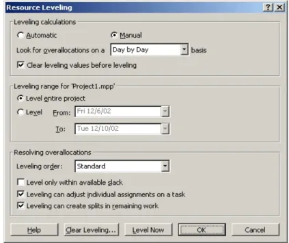
1.4 Microsoft Project 2007 . . . 10
1.5 Microsoft Project, two-task problem example . . . 11
1.6 Sciforma Corporation PS8 . . . 11
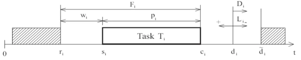
2.1 Graphic representation of task parameters . . . 15
2.2 Two tasks with generalized precedence constraints . . . 17
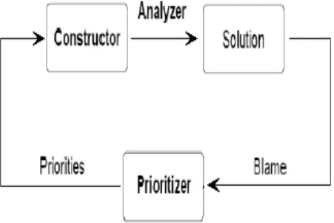
3.1 Construct/Analyze/Prioritize cycle . . . 19
3.2 Example task-on-node graph . . . 20
3.3 The first SWO iteration schedule . . . 21
3.4 The second SWO iteration schedule . . . 22
3.5 The third SWO iteration schedule . . . 22
4.1 Initial priorities calculation . . . 26
4.2 Two tasks with generalized precedence constraints . . . 27
4.3 ESTi calculation, predecessors order . . . 29
4.4 LSTi calculation, successors order . . . 29
4.5 Bulldozing method example, task-on-node graph . . . 31
4.6 Bulldozing method example . . . 31
4.7 Bulldozing method example . . . 32
4.8 LeftBulldozing method example . . . 34
5.1 The Project Management Triangle . . . 40
5.2 Example 5.1: resource Group A overallocation . . . 42
5.3 Example 5.1: resource Group B overallocation . . . 43
5.4 Example 5.1: Group A, Resource Leveling function result . . . 43 ix
5.7 The GanttProject structure . . . 47
5.8 The relationship between the ResourceLevelingAction class and the Re-sourceLevelingAlgorithm class . . . 51
5.9 The call sequence between the ResourceLevelingAction class and the Re-sourceLevelingAlgorithm class . . . 52
5.10 Involving the new classes into GanttProject structure . . . 53
5.11 Create a new project from CVS . . . 54
5.12 Checkout the project from CVS repository . . . 55
5.13 Running GanttProject . . . 56
5.14 Microsoft Project, two-task problem example . . . 57
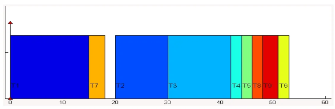
5.15 MS Project 2007, Resource Leveling function example . . . 57
5.16 GanttProject, Resource Leveling function example . . . 58
6.1 Progen/Max . . . 60
6.2 Scheduling Algorithm Tester . . . 62
6.3 The Cmax comparison . . . 63
6.4 The Cmax comparison with higher percentage of maximal time lags . . . 63
6.5 The Cmax comparison of ALG and modified ALG for high scale problem instances . . . 64
6.6 The CP U timecomparison . . . 65
6.7 The CP U timecomparison with higher percentage of maximal time lags 65 6.8 The CP U time comparison of ALG and modified ALG for high scale problem instances . . . 66
Abbreviation
Term
BaB Branch-and-Bound
CPU Central Processing Unit
CVS Concurrent Versions System
GUI Graphical User Interface
GPL General Public License
ILP Integer Linear Programming
JDK Java Development Kit
JRE Java Runtime Environment
MS Microsoft
RCPSP Resource-Constrained Project Scheduling Problem
RLP Resource Leveling Problem
SWO Squeaky Wheel Optimization
Notation
Term
Cmax Makespan - total project length
EST Earliest Task Start Time
LST Latest Task Start Time
m Number of resources
n Number of tasks
p Task processing times
S Task start times
T Task
W Precedence matrix with general precedence constraints xii
Introduction
1.1
Motivation
Nowadays, scheduling becomes more and more important part of our life. Many people face scheduling problems every day, e.g. at the airport (someone is responsible for assign-ing the planes to gates), in the hospital (creatassign-ing nurse worksheets), at the constructions (creating workers worksheet, construction process plan) and so on. In general, scheduling
is the process of assigning a set of tasks (or commonly called jobs) to a set of resources (humans, machines, processors, etc). The result is a timetable, schedule or plan. Before defining scheduling more precisely, let us give an intuition about typical applications.
One of the typical applications is Project management. Project management is a process of organizing and managing resources to achieve a specific goal (e.g. minimizing total project length, minimizing total cost, etc). A project might be a building construc-tion, a chemical process or a computer system implementation.
Scheduling also plays an important role in computer science. The fast expansion of use of computers in public and private sector not only provided a tool to practically solve scheduling problems, but also created a new source of these problems itself: problems that arise in computer control (e.g. software scheduling problems, parallel processing, computer networks etc).
As we mentioned before, there are typical scheduling applications, each of this applica-tions contains scheduling problems that need to be solved. To find a solution, scheduling algorithms are used. The result is the schedule that achieves required goal. This the-sis is concerned about implementation of An Effective Algorithm For Project Scheduling With Arbitrary Temporal Constraints (Smith a Pyle, 2004), which is a scheduling
rithm solving mostly project management problems, where total project length needs to be minimized. The algorithm has been implemented and modified in Mathworks Mat-lab environment. The modifications have been done in order to increase the algorithm speed at the price of its less efficiency. The modified algorithm has been implemented into GanttProject (http://ganttproject.biz/), which is a Java based open-source project manager software.
1.2
Problem statement
The scheduling problem is given by a list of tasks, a list of precedence constraints and a list of available resources. Problem should be represented by task-on-node graph1 (see Figure 1.1).
Figure 1.1: Task-on-Node graph There can be two types of precedence constraints:
• The (classic) precedence constraints (shown in Figure 1.1), constraints where each arc between two nodes is weighted by 1. They represent only an existence of rela-tionship between two tasks (exists or not) without information about relarela-tionship characteristics.
• The generalized precedence constraints represent as well relationship existence as relationship characteristics.
1Graph where tasks are represented by nodes and dependencies between tasks are represented by
Assuming a generalized precedence constraints, there can be two edge types:
1. The forward edge, the edge from node Ti to node Tj with positive time lag wij. It
indicates that Tj must start at least wij time units afterSi (start time of taskTi).
2. Backward edge, the edge from node Tj to node Ti with negative time lag wji. It
indicates that Sj must be no more thanwji time units afterSi.
The objective is to find a schedule with minimal makespan (Cmax)2 satisfying task
durations and relations, and resource constraints.
Example 1.1: Building a house
The table below shows a simple project plan for building a house (note that task durations are not real).
Task number Task Duration General precedence constraint 1 Foundations 15 days
2 Walls 10 days Starts at least 5 days after finishing the foundations (task 1).
3 Roof 12 days Starts after finishing the walls (task 2).
4 Doors and windows 2 days Starts after finishing the roof (task 3).
5 Cross buntons 2 days Starts after finishing the doors and windows (task 4).
6 Kitchen 2 days Starts at least 3 days after starting the cross buntons (task 5).
7 Bedroom 3 days Starts no more than 4 days after start building the kitchen (task 6). 8 Bathroom 2 days Starts at least 2 days after starting
the cross buntons (task 5).
9 Living room 3 days Starts at least 3 days after starting the cross buntons (task 5).
The problem representation could be rewritten to task-on-node graph with generalized 2C
precedence constraints.
Figure 1.2: Example: Building a house, task-on-node graph
The objective is to find a schedule minimizing total project length with respect to gener-alized precedence constraints. The solution of our problem could be represented by the schedule shown in Figure 1.3.
Figure 1.3: Example: Building a house, resulting schedule
The problem is referred to NP-hard class problems which means that no polynomial time algorithm3 exists for its solution. There are three approaches to solve NP-hard
problems:
1. Algorithms like Branch-and-Cut or Branch-and-Bound, which find an optimal so-lution at the expense of worst-case computation time4.
3Polynomial time algorithm is an algorithm, where its computational time is in worst case upper
bounded by polynomial function of the input problem size.
2. Heuristic algorithms are used to find a solution among whole solution space, but they do not guarantee that the found solution is the best one. They work with respect to the computation time.
3. Approximation algorithms work in polynomial time, but there is no guarantee that the found solution is optimal. The only guarantee is that relative error between approximation algorithm solution and optimal solution is lower than a certain co-efficient.
The primary goal of this work is to find and implement the most suitable algorithm to minimize the total project length, with respect to generalize precedence constrains between tasks. This problem is known as the Resource-Constrained Project Scheduling Problem with Arbitrary Temporal Constraints (RCPSP/max). There have been many scheduling algorithms solving RCPSP/max. We decided for An Effective Algorithm for Project Scheduling With Arbitrary Temporal Constraints which is a heuristic algorithm invented by Tristan B. Smith and John M. Pyle (2004). At the core of selected heuristic is a Squeaky Wheel Optimization (Joslin a Clements, 1998) method with an effective resolution mechanism called Bulldozing. Selected method is competitive to Branch-and-Bound (BaB) and Integer Linear Programming (ILP) algorithms. It consistently solves all feasible problems with respect to algorithm computation time, which is mostly lower than above mentioned methods.
1.3
Related work
Related work can be characterized along two dimensions: scheduling algorithms and scheduling tools.
1.3.1
Scheduling algorithms
As we mentioned before, the problem consists of a set of activities and a set of renewable resources. All algorithms assume that resource capacities, activity processing times and activity dependencies are fixed throughout project, and the objective is to minimize the total project duration (makespan). Preemption is not allowed. Previous research on algorithms solving RCPSP/max problem uses mathematical programming techniques
and implicit enumeration, e.g., linear programming and branch-and-bound. Nowadays, when project scale is growing, heuristic algorithms are more interesting.
1.3.1.1 Branch-and-Bound algorithms
There have been developed various branch-and-bound algorithms to find an optimal solu-tion. There are different branching and pruning methods used to solve the RCPSP/max problem. The static RCPSP has been extensively studied by Brucker (1998). A major difficulty in this problem is to maintain the resource limitation over the horizon time.
A Branch-and-Bound Algorithm for a Single-machine Scheduling Problem With Pos-itive and Negative Time-lags (Brucker et al., 1999) shows that complex scheduling prob-lems can be reduced to the problem of scheduling tasks with arbitrary time-lags given by relations on a single-machine. The second part introduces the branch-and-bound al-gorithm for solving single-machine problem.
A Branch-and-Bound Procedure for the Generalized Resource-Constrained Project Schedul-ing Problem (Demeulemeester a Herroelen, 1997) is based on a depth-first solution strat-egy that solves resource capacity violations by delaying a minimal subset of activities. Nodes in the solution tree represent resource and precedence feasible partial schedules. Branches coming from a parent node correspond to minimal combinations of activities, the delay of which resolves resource conflicts at each parent node. Precedence based lower bound and two dominance rules (left-shift rule, cutset rule) are introduced in order to restrict the growth of the solutions tree.
1.3.1.2 Linear programming
Scheduling with Start Time Related Deadlines (Sucha a Hanzalek, 2004) is based on integer linear programming method. The algorithm complexity is not polynomial but method is able to find an optimal solution.
Linear programming based algorithms for preemptive and non-preemptive RCPSP
(Damay et al., 2007). The algorithm uses variables associated to subsets of independent activities that can be processed simultaneously. These activities are called antichains. Precedence and non-preemption constraints are represented by antichains and eliminated by the linear formulation.
1.3.1.3 Heuristics
Local Search Algorithms for a Single-Machine Scheduling Problem with Positive and Negative Time-Lags (Hurink a Keuchel, 2001) is a local search algorithm where basic method is a tabu search approach which starts with an ’infeasible’ sequence of the jobs and tries to guide the search to a feasible sequence. This method can be considered as general metaheuristic and mostly succeeds in feasible solution. One of the biggest disad-vantages of this algorithm is that the computational times are very often high.
In an article,Self-Adapting Genetic Algorithms with an Application to Project Schedul-ing (Hartmann, 1999), genetic algorithm is presented using mechanisms or processes such as selection, crossover and mutations, similar to Darwinian natural selection biological model. The goal is to produce a better solution by selecting only the best existing solu-tions and their recombination.
Squeaky wheel optimization (Joslin a Clements, 1998) is an iterative search technique for solving optimization problems. A solution is constructed by a greedy algorithm based on the priorities assigned to all elements of the problem (elements with higher priority are handled earlier). Constructed solution is then analyzed and elements priorities are changed. The result of this analysis is a new priority order used by the greedy algorithm to construct the next solution. This Construct/Analyze/Prioritize cycle continues until some accepted or required solution is found.
A Constraint-Based Method for Project Scheduling with Time Windows (Cesta et al., 2000). At the core of the algorithm is a Constraint satisfaction problem solving (CSP) search procedure, which generates a set of task start times and removes resource conflicts from otherwise temporary feasible solution. This is done by a conflict sampling method that selects conflict sets involving tasks with higher capacity requests.
The article, A Competitive Heuristic Solution Technique for Resource-Constrained Project Scheduling (Tormos a Lova, 2001), presents heuristic approach, based on multi-pass method, combining random sampling procedures with backward-forward method. The algorithm component parameters are specified through a step-wise computational analysis.
1.3.2
Scheduling tools
In this work, when we talk about scheduling tools, we mostly mean project management software that uses scheduling algorithms to perform a Resource Leveling5 function.
Microsoft Project 2007 (http://office.microsoft.com/project) is a proprietary, widely used project management software. Optimization of the project schedule is done by man-ually assigning a priority number to a task. MS Project allows user to set resource leveling properties (see Figure 1.4). The most important property is ’Leveling order’ that deter-mines how will scheduling algorithm treat with tasks and in which order.
Figure 1.4: Microsoft Project 2007 There are 3 possibilities:
• ID Only - algorithm delays tasks with higher Task ID first before looking at lower IDs.
• Standard - algorithm examines following criteria in this order: predecessor relation-ship, slack, dates, priorities, constraints.
• Standard and Priority - same as Standard, but uses priorities as primary factor.
Even though, Microsoft Project is very popular and prestige software, it is unable to bind two tasks with forward and backward edge all at once (see Figure 1.5).
Figure 1.5: Microsoft Project, two-task problem example
Sciforma Corporation PS8 (http://www.sciforma.com/) is proprietary project management software. It allows to set resource leveling properties, and to specify both project and task priorities for use in resource leveling. It also allows to define margins for each resource that determine what conditions constitute an overload.
Figure 1.6: Sciforma Corporation PS8
Open Workbench(http://www.openworkbench.org/) is an open-source project man-agement software. The main difference between Microsoft Project and Open Workbench is that Microsoft Project leveling resource algorithm is only shifting overloaded tasks on the schedule to find the next contiguous window in which the resource can complete the entire task. In Open Workbench, the resource leveling algorithm calculates the whole schedule from the beginning. Although, it is an open-source software, scheduling algo-rithms are currently not open sourced.
1.4
Contribution
BaB or ILP algorithms find always an optimal solution of RCPSP/max. However, they are not able to find an optimal solution for a large scale scheduling problems. Therefore heuristic algorithms are used. Their computational times are very often less than BaB or ILP algorithms but on the other side, they often leads to loss of finding the best solution. Heuristic mostly find a near optimal solution in polynomial time.
The thesis primary object is to implement An Effective Algorithm for Project Schedul-ing with Arbitrary Temporal Constraints which is heuristic based on Squeaky Wheel Optimization and resolution method called Bulldozing. Selected heuristic will be imple-mented into Mathworks Matlab environment and into an open-source project, GanttPro-ject. GanttProject is the project manager software working under GPL6. It will be
extended for a new function called Resource Leveling which will improve application us-ability closer to commercial software like MS Project. All source-codes will be uploaded to GanttProject CVS7 server, hosted at SourceForge(http://sourceforge.net/), and will
be a part of the future version.
Outline of this thesis. The thesis is divided into six chapters. To give a concise overview, let us summarize the contents of the individual chapters:
CHAPTER 1: Provides a brief introduction to project scheduling, problem statement and related works.
CHAPTER 2: This chapter gives a detailed introduction to RCPSP/max. It contains problem description and also introduces basic scheduling theory notions like task, process-ing time, release date,Cmax, etc.
CHAPTER 3: Describes closely Squeaky Wheel Optimization approach.
CHAPTER 4: Here, individual parts of selected algorithm are analyzed. It is divided into two sections. The first one introduces main algorithm parts: Squeaky Wheel opti-mization as a part of an implemented algorithm, Bulldozing and Refilling methods. The second one concerns about own algorithm modifications that lead to enhancement its
6General Public License 7Concurrent Versions System
performance.
CHAPTER 5: This chapter gives an information about GanttProject structure and about own implementation of the scheduling algorithm as a Resource Leveling method.
CHAPTER 6: Chapter six presents an experimental results of the implemented algo-rithm and its modification.
Resource-Constrained Project
Scheduling Problem with Arbitrary
Temporal Constraints
(RCPSP/max)
2.1
Introduction to scheduling
Before defining RCPSP/max more closely, let’s introduce some basic scheduling theory terms that are used throughout the thesis.
One of the most important term is Task (or sometimes called Activity). Graphic representation of task and its paremeters is shown in Figure 2.1.
Figure 2.1: Graphic representation of task parameters Tasks are characterized by following notions:
• Task processing times p = (p1, p2, . . . , pi, . . . , pn). Concern about how long are
individual tasks processed without interruption. 15
• Ready times r = (r1,r2, . . . , ri, . . . , rn). Express time where each task is ready to
be processed.
• Due dates d = (d1, d2, . . . , di, . . . , dn). Due dates specify times when each task
should be finished. If task is finished later than its due date, some penalization is imposed (e.g. increase production costs).
• Deadlines ˜d= (d˜1,d˜2, . . . ,d˜i, . . . ,d˜n). In comparison to due dates, deadlines specify
times when each tasks must be finished otherwise the scheduling is assumed to be failed.
• Priorities w= (w1,w2, . . . ,wi, . . . ,wn). Concern about task priority with respect
to other tasks (e.g. one task must be scheduled before another).
For each task, there are additional parameters, used like a criterion for resulting schedule classification:
• Completion time Ci. Time when task is truly finished.
• Flow time Fi = Ci - ri. Represents total task processing time, including task’s
waiting.
• Tardiness Di = max(Li,0). Non-zero value indicates overrun required due date.
• Earliness Ei = max(-Li,0). Non-zero value indicates that task has been finished
earlier than required due date.
We have introduced terms like task and its parameters. Now let’s introduce some crite-rions along which resulting schedules are optimized:
• Makespan (total schedule length):
Cmax = max{ci}
• Maximum lateness:
• Mean flow time: ¯ F = 1 n n X i=1 Fi
• Mean weighted flow time:
¯ F = n P i=1 Fi n P i=1 wi • Mean earliness: ¯ E = 1 n n X i=1 Ei
2.2
RCPSP/max problem
RCPSP/max problem contains a set {T1, ...,Tn} of tasks and a set {R1, ...,Rm} of
re-sources. Each task Ti has its start time Si and a processing time pi. Each resource has
its maximum capacityckand execution of each task Ti requires an amountrik of resource
k for each time unit of execution. There are two types of constraints:
Precedence constrains mean that the start time of each task is related to the start time of another task. There are two types of generalized precedence constraints:
1. Positive time lags wij, from task Ti to taks Tj, indicates that Si must be at least
wij time units after Sj.
2. Negative time lags wji, from task Tj to taks Ti, indicates that Sj must be no more
Figure 2.2: Two tasks with generalized precedence constraints Precedence constrains can be summarized as follows:
min w≤ i,j Sj −Si ≤ max w i,j
Resource constraintsrepresent maximum capacity of each resource. Resource constraints can be summarized as follows:
X
{i|Si≤t≤Si+pi}rik ≤ck,∀t,∀k
A schedule can be considered as an assignment of start time Si to each task Ti. It is
time-feasible if it satisfies all precedence constraints and isresource-feasible if it satisfies all resource constraints. A schedule satisfying both time-feasible and resource-feasible constraints isfeasible. The goal of an RCPSP/max problem is to find a feasible schedule minimizingCmax = max(Si+pi). Minimizing theCmax is not the only one criterion while
solving the RCPSP/max problem. Cmaxis always bound with tasks and their start times.
Sometimes there is a need for criteria, where the objective function does not depend on how the individual activities are scheduled, but on how they are combined in order to use the resources. For this purpose, the Resource Leveling Problem (RLP) criterion is used. RLP minimizes:
• The total squared utilization cost of all resources.
• The total overload cost (loading the resourceRk over its capacityck incurs the total
overload cost).
RCPSP/max is referred to the NP-hard class problems. It means that no polynomial time algorithm exists for this problem.
Squeaky Wheel Optimization
3.1
Squeaky Wheel Optimization
Squeaky Wheel Optimization (SWO) is an iterative search technique for solving opti-mization problems. A solution is constructed by a greedy algorithm with priority scheme. When constructing a solution, greedy algorithm is making its decision based on priori-ties assigned to all elements of the problem1 (elements with higher priority are handled earlier). Constructed solution is then analyzed and elements priorities are changed. The result of this analysis is a new priority order, used by the greedy algorithm to construct the next solution. This Construct/Analyze/Prioritize cycle (see Figure 3.1) continues until some accepted or required solution is found.
Figure 3.1: Construct/Analyze/Prioritize cycle
1In scheduling domain, those elements are referred to tasks. 19
Squeaky wheel optimization can be split into three parts: Constructor
The constructor adds elements, one at a time, into schedule based on priority order. Priorities are arranged in increasing order which means that elements with higher priority are handled by constructor earlier.
Analyzer
The analyzer analyzes the solution created by the constructor and tries to find trouble elements (elements that are hard to schedule or don’t respect task constrains). After find-ing trouble elements, the “blames” are assigned. The analyzer calculates a lower bound on the minimum possible cost (minimum worthiness that task extends actual makespan) that each task could contribute to schedule. The blame assigned to each task is the difference between its actual cost and a minimum possible cost. In other words, priorities of trou-ble elements are increased much more than non-troutrou-ble elements. In the next algorithm iteration, trouble elements (or hardly scheduled tasks) are handled by constructor earlier.
Prioritizer
Once the blame has been assigned, the prioritizer modifies the previous sequence of elements by moving tasks with higher blame into the front of sequence. The higher the blame, the further the element is moved.
Example 3.1: Squeaky wheel optimization
Let’s have a look at simple example for better understanding Construct/Analyze/Prioritize cycle. The problem is represented by task-on-node graph shown in Figure 3.2.
Figure 3.2: Example task-on-node graph task processing times: p1 = p2 =p3 = 1
precedence constraints:
T1 must start at least 2 time units beforeT2
T2 must start at least 2 time units before T3
The first SWO iteration:
Construction
Construction task order (based on task priorities) is (T3, T2, T1).
Figure 3.3: The first SWO iteration schedule
Analyze:
Schedule is not feasible.
Based on precedence constraints, T1 must be placed at least 2 time units before T2 (S1’
= -1) and T2 must be placed at least 2 time units before T3 (S2’ = -2)
Blames(T1) = S1 - S1’ = 2 - (-1) = 3
Blames(T2) = S2 - S2’ = 1 - (-2) = 3 Blames(T3) = S3 - S3’ = 0
newPriorities(T1) = Priorities(T1)+ Blames(T1) = 1 + 3 = 4
newPriorities(T2) = Priorities(T2)+ Blames(T2) = 3 + 2 = 5
newPriorities(T3) = Priorities(T3)+ Blames(T3) = 3 + 0 = 3
Prioritize
New construction order = (T2, T1, T3).
The second SWO iteration:
Construction:
Figure 3.4: The second SWO iteration schedule
Analyze:
Schedule is not feasible.
Based on precedence constraints, T1 must be placed at least 2 time units before T2 (S1’
= -2).
Blames(T1) = S1 - S1’ = 1 - (-2) = 3
newPriorities(T1) = Priorities(T1)+ Blames(T1) = 4 + 3 = 7
newPriorities(T2) = Priorities(T2) = 5
newPriorities(T3) = Priorities(T3) = 3
Prioritize:
New construction order = (T1, T2,T3)
The third SWO iteration:
Construction:
Task order is (T1,T2,T3)
Figure 3.5: The third SWO iteration schedule
Analyze:
An Effective Algorithm For Project
Scheduling With Arbitrary
Temporal Constraints
In the Chapter 2, RCPSP/max problem has been introduced. Now, let’s have a look how to solve it. There are many approaches to solve RCPSP/max. We have decided for An Effective Algorithm For Project Scheduling With Arbitrary Temporal Constraints (Smith a Pyle, 2004). This algorithm has been chosen because of its low computation time and good solution quality. The chapter is divided into two sections. The first one deals with the algorithm fundamentals. The second one describes the algorithm implementation into Mathworks Matlab environment. The next chapter gives an introduction to project management and concerns about the implementation of the algorithm into an open-source project management software, GanttProject.
The algorithm represents a heuristic approach using an iterative method called Squeaky wheel optimization (SWO) to aim RCPSP/max problem. At the core of SWO is a greedy schedule constructor. The constructor is priority-based, which means that the tasks are placed one at time into the schedule according to their priorities (higher the priority, earlier the task is handled by constructor). Each solution is then analyzed and the pri-orities are changed in order to find a feasible solution. This cycle continues until some acceptable solution is found.
Since RCPSP/max belongs to NP-hard problems, it can happen that SWO will be ineffective and not able to find a feasible solution. Therefore, the algorithm is extended for a new conflict resolution mechanism calledBulldozing. This method is trying to
tain a partial-constructed schedule feasibility by moving the set of tasks to the later start times. After finding a feasible solution, similar methods are used to move certain sets of tasks back to earlier start times, in order to preserve schedule feasibility.
Before describing algorithm implementation, let’s briefly remind some RCPSP/max problem fundamentals introduced in Chapter 2:
The problem contains a set {T1, ...,Tn} of tasks and a set {R1, ...,Rm} of resources.
Each activity Ti has its start time Si and a processing time pi. Each resource has a
maximum capacityck and execution of each taskTi requires an amount rik of resource k
for each time unit of execution. Precedence constrains:
Si+wij ≤Sj
Resource constraints:
X
{i|Si≤t≤Si+pi}rik≤ck,∀t,∀k
The main goal is to minimizeCmax = max(Si+pi) representing the total schedule length.
The resulting schedule has to be feasible which means that it has to satisfy all precedence and resource constraints.
4.1
Algorithm Implementation
At first, let’s give an general overview and then explain certain algorithm features more closely.
As it was mentioned before, SWO is an iterative search technique for solving optimiza-tion problems. It means that soluoptimiza-tion is found after minimal Construct/Analyze/Prioritize cycles (iterations). In each iteration, the constructor (represented by the ScheduleWith-Dozing(Ti,X1) method) selects a start time for each unscheduled task from a time
win-dow [ESTi, LSTi] (ESTi - Eearliest Task Start Time, LSTi - Latest Task Start Time).
Each window represents all time points between the earliest and latest start time we 1whereX is a set of tasks that need to be moved by the Bulldozing method
wish to consider, and is initialized to [0, horizon-pi], where initial horizon is the goal
makespan. When [ESTi, LSTi] interval is selected then PlaceTask(Ti,t) places task Ti
into theScheduleat a time pointt. Iftis later thanLSTi,Bulldozing method is invoked.
If there has been still no feasible start time selected, then Ti is placed at ESTi and is
marked as unfeasible. After exploring all tasks, resulting schedule is analyzed, blames are assigned and priorities are updated. When a feasible solution is found, LeftShifting method is trying to move all tasks to earlier start times in order to preserve feasibility. After finding a feasible solution, makespan is counted and compared to the previous so-lution. If the new solution is better then the previous one, the new solution is saved and kept by the algorithm.
An algorithm general overview can be summarized in the following pseudo code: 1: M Kbest = infinity
2: horizon = goal makespan
3: initialize all P riorities
4: for 1 to M axIter
5: for 1 to n
6: Ti - get unscheduled task with the highest priority
7: X = { } 8: if ScheduleWithDozing(Ti,X)fails 9: f easible = FALSE 10: end 11: if feasible 12: LeftShifting(Schedule)
13: if (M Kcurrent less than M Kbest)
14: M Kbest = M Kcurrent
15: decrease horizon
16: if 10 iteration without feasible solution 17: increase horizon
18: update P riorities
19: end
al-gorithm is able to find a feasible solution without priorities initialization, the proper initialization can help to find a feasible solution faster. Each P riority(Ti) is initialized
to 10 x LSTi value, calculated by the temporal constraint propagation (Caseau, 1997).
Before LSTi calculation, the problem is transformed into the task-on-node graph with
general precedence constraints. This graph is then used as an input argument for the
Floyd-Warshall algorithm (Demel, 2002) which returns the longest path between each two nodes (tasks) in a weighted, directed graph (task-on-node graph).
Figure 4.1: Initial priorities calculation
Now, let’s describe individual methods more closely: The ScheduleWithDozing method
Before describing the ScheduleWithDozing method, some basic scheduling terms will be remembered, and a Precedence matrix (with general precedence constraints) will be introduced:
• Task processing times p = (p1, p2, . . . , pi, . . . , pn). Concern about how long are
individual tasks processed without interruption.
• Task start times S = (S1, S2, . . . , Si, . . . , Sn). Specify the task processing start
• Precedence matrix with general precedence constraints W W= w11 w12 w12 w22 . . . . . . w1j w2j . . . w1n . . . w2n .. . ... ... ... wi1 wi2 . . . wij . . . win .. . ... ... ... wn1 wn2 . . . wnj . . . wnn
The matrix represents how the each task start time pi is related to the start time
of another tasks pj (see Figure 4.2).
Figure 4.2: Two tasks with generalized precedence constraints
At the beginning, the function calculates a time window domain [ESTi,LSTi] for the
specified task Ti. This bounds (ESTi,LSTi) are calculated using the task start times
vector p and the precedence matrixW. When the time window domain [ESTi,LSTi] is
determined, the algorithm is exploring all time slots in the schedule in an effort to find a free resource-feasible time slot for starting the task Ti. If none is found, Bulldozing
method is invoked. Bulldozing allows the greedy constructor to move the sets of tasks
X later in a partial schedule to maintain feasibility. After a successful bulldoze, the
LeftBulldozing method is trying to move the same sets of tasks back to the earlier start times. If bulldozing fails and none resource feasible time slot has been found, resource constraints are neglected, and the task Ti is placed at the earliest start time ESTi. The
The ScheduleWit hDoz ing(Ti,X)method pseudo code is shown below:
1: t = earliest resource-feasible time for Ti in [ESTi,LSTi(orig)]
2: if (t ≤ LSTi)
3: PlaceTask(Ti,t)
4: else if (t more than LSTi) % Bulldozing method is invoked
5: PlaceTask(Ti,t)
6: Tj = tasks that need to be moved to preserve schedule feasibility
7: X = X ∪ {Tj}
8: Y = X
9: while (Y is NOT empty)do
10: Tk = randomly selected task from the set X
11: UnplaceTask(Tk) 12: X =X - {Tk} 13: ScheduleWithDozing(Tk,X) 14: end 15: LeftBulldozing(Y) 16: else 17: PlaceTask(Ti,ESTi)
18: Undo All Bulldozing 19: feasible = FALSE
20: end
ESTi calculation
For task Ti, all predecessors Tj are checked whether they are scheduled or not.
If yes, then:
ESTi = max (ESTi, S(Tj) + w(Tj,Ti)).
Figure 4.3: ESTi calculation, predecessors order
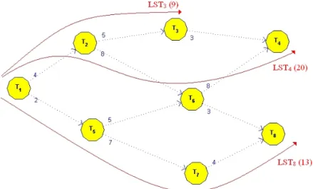
LSTi calculation
For task Ti, all successorsTj are checked whether they are scheduled or not.
If yes, then:
LSTi = min (LSTi, S(Tj) - w(Ti,Tj)).
The predecessors (in the matrix W) are examined in the order shown in Figure 4.4.
Figure 4.4: LSTi calculation, successors order
The Bulldozing method
For highly constrained problems the SWO greedy algorithm is unable to find a feasible schedule. This problem is mostly occurred because of existence of the maximum time lags (the negative time lags between two nodes). Without maximum time lags, a greedy algorithm can find always a feasible schedule, because each task Ti can be postponed as
long as it is necessary to conserve resource availability. Using the maximum time lags, the taskTi can not be postponed long enough, if the tasks that constraints Ti have been
scheduled too early. The main idea of bulldozing is to delay the set of tasksX constrain-ing Ti, so that Ti can be scheduled in the postponed time.
TheBulldozing method is invoked when the taskTican not be scheduled in the current
[ESTi,LSTi] time window domain. Bulldozing considers a larger time window domain to
find a free time slot in the schedule for placing the task Ti. It extends the [ESTi,LSTi]
time window domain to [ESTi,LSTi(orig)], where LSTi(orig) is the latest start time of the
taskTi when no other activities are scheduled. If bulldozing finds a free time slot (at the
timet) for taskTi outside the [ESTi,LSTi] window but within the [ESTi,LSTi(orig)], the
taskTi is placed at the timet. After placing the taskTi, algorithm finds all tasksTj that
constrain task Ti and places them into the set X (which is the set of all tasks that need
to be moved). Each taskTk that is randomly selected from the set X, is taken out from
this set, unplaced and the algorithm is trying to find a new feasible start time for the taskTk using the recursive call ofScheduleWithDozing(Tk,X). If all tasks from setX are
scheduled feasible then bulldozing success. Otherwise, all delayed tasks Tk from the set
X revert to their previous position (position before invoking bulldozing).
One of the main advantages of the Bulldozing method is its recursive nature, which means that more tasks can be moved than the original set X forced by task Ti. Each
task Tk from the set X can also force another set of tasks X0. From a broader point of
view, we can say that each bulldozed taskTi forces sub-sets of highly constrained tasks.
These sub-sets will be moved to later start times until all sub-sets precedence constraints are satisfied. This approach is very interesting because it is able to divide problem into the sub-problems. Each sub-problem is then solved separately and these partial solutions are then combined into the overall solution.
Example 4.1: The Bulldozing method
The purpose of this example is to better explain the Bulldozing method. Let the example consist of four tasks with the following precedence constraints:
• Task T4 can start at least 5 time units after starting the task T1.
• Task T4 must start no more then 3 time units after starting task T2.
• Between all other tasks there are no precedence constraints.
The problem could be also presented by task-on-node graph shown in Figure 4.5:
Figure 4.5: Bulldozing method example, task-on-node graph
Consider that tasks T1,T2 and T3 have been scheduled within the following time domain windows:
EST1(orig)=EST1=0, LST1=10 EST2(orig)=EST2=1, LST2=10 EST3(orig)=EST3=2, LST3=10
Now, we are trying to schedule T4 inside a time window domain EST4=5, LST4=4. The constructor is unable to find a resource feasible time slot in the schedule. Therefore the LST4 is updated to LST4(orig)=10 and the constructor is trying to examine the
fea-sible schedule once again. Now, the constructor has found a free time slot at time t=5. The task is scheduled at t=5 apart from maximum time lags between tasks T2 and T3
(see Figure 4.6).
Figure 4.6: Bulldozing method example
Bulldozing method finds all tasksTj causing unsatisfied (maximum time lags) constraints
Constraining tasks are: T2,T3
Update the set X: X ={T2,T3}
After unscheduling the tasks (one at time) {T2,T3}, the time domains for each task T2
and T3 is updated: EST2=3, LST2=10 EST3=4, LST3=10
After the successful bulldoze (moving all tasks form the set X to the later start times), the resulting schedule in Figure 4.7 is feasible and all general precedence constraints are satisfied.
Figure 4.7: Bulldozing method example
The LeftBulldozing method
However, bulldozing finds almost always a feasible solution (if exists), this solution is often not optimal. The LeftBulldozing method is trying to reduce the scheduleCmax and
helps to find an optimal solution. After a successful bulldoze, the same set of tasks X, that have been moved by bulldozing, is tried to be moved by leftBulldozing back to the earlier start times. This approach is also Bulldozing, because we are trying to move the sub-sets of tasks that are highly constrained among themselves.
The leftBulldozing is the same as scheduleWithDozing except for these three differences: • On line 1, the range tried is [ESTi(orig),LSTi] (ie we try placing the task earlier
than it can currently go, not later). We assume that ESTi(orig) is a counted ESTi
before running bulldozing.
• On line 2, we instead uset ≥ESTi.
The LeftBulldoz ing(X) method pseudo code is shown below: 1: Ti = the first task from the setX
2: X = X -{Ti}
3: t = earliest resource-feasible time for Ti in [ESTi(orig),LSTi]
4: if (t ≤ ESTi)
5: PlaceTask(Ti,t)
6: Tj = tasks that need to be moved to earlier start time
7: Y =Y ∪ {Tj}
8: while (X is NOT empty)do
9: Tk = randomly selected task from the set Y
10: UnplaceTask(Tk)
11: Y = Y - {Tk}
12: LeftBulldozing(Tk,Y)
13: end
14: if (t > LSTi)
15: Undo All LeftBulldozing 16: feasible = FALSE
17: end
Example 4.2: The LeftBulldozing method
Let’s have a look at the previous example and try to perform the LeftBulldozing method to the resulting schedule. Even though, the purpose of the LeftBulldozing method is to reduce the schedule makespan, this approach rarely works. Because of this, the ex-ample mainly shows how to count the ESTi(orig) for tasks that are left bulldozed.
After a successful bulldoze of the tasks T2 and T3, leftBulldozing is trying to move the
same set of tasks back to the earlier start times. At first, the ESTi time domains are
updated to:
EST2=EST2(orig)=1, LST2=10 EST3=EST3(orig)=2, LST3=10
Applying the LeftBulldozing method, the resulting schedule (in Figure 4.8) hasn’t change compared to the resulting schedule produced by the Bulldozing method.
Figure 4.8: LeftBulldozing method example
The LeftShifting method
After finding a feasible solution (schedule), this method is trying to reduce the schedule makespan. The main idea of this method is to left-shift tasks that can take an advan-tage of resources vacated by bulldozed activities. Simply said, this approach is trying to move each task Ai, for which holds start timeSi> ESTi, to the left as much as possible.
The algorithm explores start times Si of all tasks (in order they were scheduled) and
counts appropriate ESTi. If Si > ESTi then the task is moved to the earlier start time
as much as possible.
The Left Shift ing(S ched ule) method is represented by the following pseudo code: 1: for 1 to n
1: t = earliest resource-feasible time for Ti in [ESTi,LSTi]
2: if (t < Si)
3: PlaceTask(Ti,t)
The Priorities update
The priorities are updated at the end of each algorithm iteration. This is a very important phase, because it strongly affects the construction task order in the next al-gorithm iteration. The main idea of priorities updating is to increase priorities to all not-scheduled tasks by a constant amount. All other tasks priorities are increased by a smaller amount with a small probability. Doing these two steps, we ensure that in each iteration, at least one task will have its priority changed.
In our implementation, following priorities-increase constants are chosen:
• An amount, how much more the task priority is increased, when the task has been scheduled = 2
• An amount, how much more the task priority is increased, when the task could not been scheduled = 4
• A probability, with which the task priority is increased, when the task has been scheduled = 0.01
4.2
Own Algorithm Modifications
Even thought, the implemented algorithm shows a very good benchmark results (shown in the Chapter 6), there are some modifications that can be done to increase its perfor-mance. The main impact of these changes is to decrease algorithm computational time on the assumption, that the resulting makespans of the original and modified algorithm are nearby equal. This can be done in two ways:
• By modifying the prioritization phase or more precisely, to change the idea of up-dating the priorities.
• By exchanging the certain algorithms for the simpler ones with nearby the same result.
4.2.1
Prioritization phase modifications
The main purpose of the algorithms solving the RCPSP/max is to find an appropriate construction order in which the tasks are scheduled feasibly. The schedule, constructed in this order, should also minimize theCmax criterion. Therefore, the prioritization phase
is very important because it strongly influences the next iteration constructor task or-der. Compared to the original implementation, the main change is that priorities are not updated in the end of each iteration, but they are update continuously in the bull-dozing part of the ScheduleWithDozing method. The main idea is that task Ti, that
needs to be bulldozed, forces another tasks Tk (all tasks in the set X) to be moved to
the later start times. All tasks Tk from X are then feasibly rescheduled; videlicet these
tasks, for conserving the schedule feasibility, must be in the construction order later than
Ti. Therefore, the best what way to update the priorities is to make sure, that in the
construction order, all tasks Tk ∈ X are later than Ti. Notice, that we do not do the
difference between the tasks in the set X. We can afford it, because the tasks Tk that
are moved by bulldozing are selected randomly (from the priorities point of view, these tasks are equal). This is done by assigning the priority values to all tasksTk less than the
priority of taskTi. We decided to decrease this value by a constant amount weighted by 2:
Priorities(Tk) = Priorities(Ti)−2
An important observation is that the correct construction order (obtained from the ap-propriate priority values), which achieves a feasible schedule, is found only in the one algorithm iteration.
This is not an only one difference. Another modification, but not as important as previ-ous one, is that at the beginning of each iteration, a random constant amount is added to each priority. This is done because it can happen, that two tasks will have the same priority and it needs to be decided which one to schedule first.
4.2.2
Reducing the code
The main idea is to exchange certain algorithms, that take a long time to be processed or their effect to the resulting schedule is not equal to their processing time. These algorithms are substituted for the simpler ones that provide nearby the same result, but using the smaller amount of CPU time. We decided for letting out the LeftBulldozing method. There are two reasons to do it:
1. It is a recursive method that is invoked every time when bulldozing success. 2. If the correct construction task order is known, we are able to schedule all tasks
once again from the beginning. Using this construction order, we will always find a feasible solution where majority part of tasks is placed to their earliest start times, which achieve the minimal makespan. This can be done without using the Left-Bulldozing method.
The leftBulldozing is then replaced by a new algorithm that originates by modifying the
LeftShifting method. The new method, in comparison to the original one, finds not only tasks that can be moved to the earlier start times, but constructs the whole schedule from the beginning using the feasible construction order. This all is done not after a successful bulldoze but at the end of each algorithm iteration.
The comparisons of the original and modified algorithm are presented in the Chapter 6.
Project Management Software,
GanttProject
5.1
Project Management
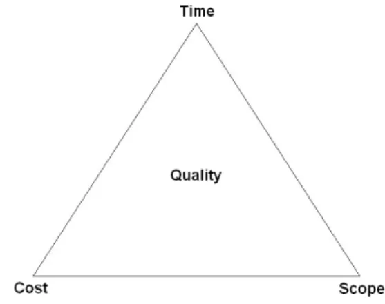
The project management is the discipline of organizing and managing the resources, with a view to achieving a specific goal (e.g. minimizing the total project cost or total project length). A project might be a building construction, implementation of new technologies into a factory or a political campaign. The project management in the modern sense began in the early 1960s, but it was also known by ancient Egyptians engineers while they were building great pyramids, that are seen still today. They had to plan how many people would be involved in specified works, how much material they would need, how much it would cost, how long it would take, etc. Nowadays, it is very similar, but the use of the project management is wider. People involved in business realized, that the properly planed projects lead to saving costs, and to the better prevention before prob-lems that could happened during the project realization. The project requirements are often summarized in a triangle (see Figure 5.1), where each vertex represents one of the following constraints: time, cost and scope.
Figure 5.1: The Project Management Triangle Each of these constraints has its own meaning:
• Time, represents the total project length. • Cost, is equal to the total project cost.
• Scope, refers to what must be done to produce the project’s end result.
The main idea is that the one side of the triangle cannot be changed without impacting the others. E.g. increasing the scope typically leads to increase of time and increase of the cost. The deal of the project management is to organize the project team in the way that will meet these constraints.
We have introduced the basics of the project management. Now becomes a question, how to plan the project in the easiest and most efficient way? The answer is, use the project management software.
5.2
Project Management Software
The project management software is an important tool for each project manager. It allows user to easily create, modify, share projects between managers, show Gantt charts1, etc. Each project consists of the set of resources, of the set of tasks and of the set precedence 1Gantt chart is a type of bar chart illustrating a project schedule (start and finish dates of the tasks,
constraints between tasks (notice, that this is the same as RCPSP/max problem). During the project planning, these tasks are created and assigned to the appropriate resources. One of the purposes of the project management software is to continuously inform the manager about the project state (e.g. gives information about total project length, task start times, task end times, critical path2 length, resource allocation, etc.). These indices
are mostly shown through Gantt charts. However, there are more important project state indices; we will take interest about resources allocation and its prevention.
Resource allocation is the process of assigning the tasks to the appropriate resources. During the project planning, it can happen that more tasks are assigned to resource then the resource is able to handle. This is calledresource overloading and it could lead to the problems during the project realization. Most of the project management software can detect and alert this problem, but in many cases it is the role of the user to maintain it. Now, you can say: “It is not so bad, just move problem tasks to the later start times..”. You are right, but what if there are more overloaded resources and more then one hun-dred tasks and precedence constraints among themselves? It is still so easy to reschedule them, considering the precedence constraints and conserving the minimal project length? The answer is “No” and therefore the good-class project management software allow user to maintain this problem using scheduling algorithms instead of manual correction.
Example 5.1: Building the house
Assume the Building the house example presented in the Chapter 1. Let’s modify it slightly:
• Suppose that there are two workers groups. The group A works on the project all the time (is able to work on all tasks). The group B is smaller then the group A and specializes only for building the rooms (e.g. living room).
• Consider, that after finishing the cross buntons, we are able to build the kitchen, bedroom, bathroom and living room simultaneously.
The table below shows a simple project plan for building a house (note that task dura-tions are not real).
2Critical path is the series of events (tasks) depending on each other and whose durations directly
Task number Task Duration General precedence constraint (assigned group)
1 (group A) Foundations 15 days
2 (group A) Walls 10 days Starts at least 5 days after finishing the foundations (task 1).
3 (group A) Roof 12 days Starts after finishing the walls (task 2).
4 (group A) Doors and windows 2 days Starts after finishing the roof (task 3).
5 (group A) Cross buntons 2 days Starts after finishing the doors and windows (task 4).
6 (group B) Kitchen 2 days Is able to start immediatelly after finishing the cross buntons (task 5). 7 (group A) Bedroom 3 day Is able to start immediatelly after
finishing the cross buntons (task 5). 8 (group B) Bathroom 2 days Is able to start immediatelly after
finishing the cross buntons (task 5). 9 (group A) Living room 3 day Is able to start immediatelly after
finishing the cross buntons (task 5). The project has been designed in Microsoft Project 2007. Figure 5.2 shows resource Group A allocation graph. Take notice of resource overallocation on 10th February.
Figure 5.2: Example 5.1: resource Group A overallocation
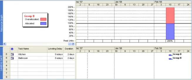
The same situation, but for resource Group B, is shown in Figure 5.3. Remark that the resource is either overallocated.
Figure 5.3: Example 5.1: resource Group B overallocation
Now, we will solve the overallocation problem using the function from the menu Tools→ Resouce Leveling. In the next two figures, we can see that the algorithm implemented in the Resource Leveling function has moved the problem tasks to the later start times in order to preserve the resources capacities.
Figure 5.5: Example 5.1: Group B, Resource Leveling function result
Understanding the Example 5.1, we should have a clear idea about resource leveling as a solution of the overallocating problem. In the next section, we will concern about an open-source management software called GanttProject and we will extend it for the scheduling algorithm (introduced in the Chapter 4) as a Resource Leveling function.
5.3
GanttProject
As we have mentioned before, GanttProject is an open-source project management soft-ware developed under the GPL license. It allows to simple create the tasks, assign them to the human resources and easily establish the dependencies between the tasks. For project control, GanttProject renders the project using two charts: a Gantt chart, displaying all tasks, dates and dependencies between the tasks; and a Load chart for resource, where all resources and their loads are shown. Here we are able to see whether some resources are overallocated or not. GanttProject is also able to print charts, generate PDF and HTML reports, exchange data with Microsoft(R) Project(TM) and spreadsheet applications3.
Although, there are many various project management applications, GanttProject offers an open-source software that is easy to learn, and is still extending its set of the basic features. Another advantage resides in its cross platform. GanttProject is a Java based application that runs on Windows, Linux, MacOSX and other operating systems supporting Java.
Figure 5.6 shows the interactions between the user and the basic GanttProject func-tions.
Figure 5.6: The basic GanttProject functions
5.3.1
GanttProject structure
GanttProject contains of 21 packages and 24 subpackages. The main project structure (without subpackages) is shown in Figure 5.7.
Figure 5.7: The GanttProject structure
In this section, we will explain only those packages and subpackages, that are in touch with our implementation (extension for the scheduling algorithm as a Resource Leveling function):
package net.sourceforge.ganttproject
Contains all general classes (e.g. classes for project variables initialization, graphical user interface (GUI), etc.).
package net.sourceforge.ganttproject.action
Includes all action listeners4 : in our case, for the GUI items (e.g. buttons).
package net.sourceforge.ganttproject.task
4Listener is the class that handles an event (e.g. after clicking the button, it calls the appropriate
This package holds the classes for the manipulation with the tasks (e.g. create or delete task, assigning the resources, task duration, task start and task end date, etc.). package net.sourceforge.ganttproject.task.dependency
Contains the classes that concern about dependencies between the tasks (e.g. type of the relationship, the weight of the edge between themselves, the set of the successors, the set of the predecessors, etc.).
package net.sourceforge.ganttproject.task.algorithm;
Covers the classes for handling the tasks events (e.g. moving tasks to another start times, critical path computation, etc.).
package net.sourceforge.ganttproject.resource
This package holds the classes for the manipulation with the resources (e.g. create or delete resource, resource load etc.).
5.3.2
Scheduling algorithm implementation
We decided to implement the scheduling algorithm, described in the Chapter 4, as the Resource Leveling function. Therefore, there is no need to explain the algorithm idea (and how it works) again. We will rather concern about mounting the algorithm in to Ganttproject as a Java environment. There are three main issues to do so:
1. Create a menu item to invoke the Resource Leveling function.
2. Create a Java class to handle the event when the Resource Leveling function is called.
3. Obtain the input data for the scheduling algorithm from the Ganttproject structure. 4. Create a Java class implementing the scheduling algorithm function.
5. Involve the newly created classes to the overall GanttProject structure. 5.3.2.1 Create a menu item to invoke the Resource Leveling function
Creating the menu item for invoking the Resource Leveling action is not a big deal. It is just adding some lines of code into the main GanttProject package, into the GanttPro-ject.java file. We have created a new item and assigned it to the appropriate menu. The next step was to “tell” the button what to do, when the user clicks on it. For this pur-pose, we used “event action handler” which is the class containing the instructions that are invoked after clicking the menu item. The last think to do was to add the “Resource Leveling” item into thei18n.properties file, which is the language database file containing all english translations for each menu item.
5.3.2.2 Create a Java class to handle the event when the Resource Leveling function is invoked
Creating the event action handler class for the Resource Leveling menu item, ResourceLevelin-gAction.java, involves addressing following three subissues:
• Obtain the input data for the scheduling algorithm from the Ganttproject structure. • Call the scheduling algorithm class with the specified input parameters.
• Use the results, returned by the algorithm, to move the tasks to start times where the resources are not overallocated.
For acquiring the data from the project, we had to decide what kind of data we would need. If we look back to the Chapter 4, we can see that the input parameters for the algorithm are: taskprocessing timesp, the precedence constraints that are represented by the matrix W and the assigned resources R. For this purpose, following methods were implemented (note, that the objective of this section is not to describe these method in detail, rather the design of the classes that need to be implemented to perform the Resource Leveling function).
• short[ ] getTaskProcessingTimes() - returns the one-dimensional array of the task processing timesp
• float[ ][ ] getW() - returns the two-dimensional array of the task processing times W
• float[ ][ ] getTaskResources() - returns the two-dimensional array of the assigned resources R
The next issue was to design how to call the scheduling algorithm. We decided to create the new class, ResourceLevelingAlgorithm.java, that implements the algorithm function. The ResourceLevelingAction class then creates a new instance of the ResourceLevelin-gAlgorithm class with the p,W and R as the input parameters. The output parameter of the algorithm specifies the task start time for each task, and the resource where each task should be processed.
Figure 5.8 shows the relationship between the ResourceLevelingAction class and the Re-sourceLevelingAlgorithm class.
Figure 5.8: The relationship between the ResourceLevelingAction class
and theResourceLevelingAlgorithm class
We have introduced both classes. Now, becomes a question. How does it work together? Figure 5.9 shows the whole call sequence.
Figure 5.9: The call sequence between the ResourceLevelingAction class
and theResourceLevelingAlgorithm class
After clicking the Resource Leveling menu item, an instance of theResouceLevelingAction class is created and the actionPerformed method invoked. ThegetTaskProcessingTimes,
getW and getTaskResources methods are called to acquire the appropriate data form the project. After this, the new instance of the ResourceLevelingAlgorithm class is created and the ResourceLevelingAlgorithmRun method, with p, W and R as the input argu-ments, is called. The result of theResourceLevelingAlgorithmRun method is then handed by the actionPerformed method of the ResouceLevelingAction class. The method moves the tasks according to the output argument (Result) of the ResourceLevelingAlgorithm-Run method, in order to prevent the resources oveallocation.
5.3.2.3 Create a Java class implementing the scheduling algorithm function
As it was mentioned before, the implemented algorithm is the same as it was closely described in the Chapter 4. While the algorithm performs the same function and uses exactly the same idea, we decided that it is not necessary to describe it once again. For those ones, who have not heard about the implemented algorithm, see the Chapter 4.
5.3.2.4 Involve the newly created classes to the overall GanttProject structure
As it was mentioned before, GanttProject contains more than twenty Java packages and subpackages. These packages are logically named and ordered by the purpose of the classes involved in each package. We decided to place the ResouceLevelingAction class
into the package net.sourceforge.ganttproject.action.resource. The ResouceLevelingAlgo-rithm class is placed in the package net.sourceforge.ganttproject.resource.algorithm.
Figure 5.10 shows the updated part of the GanttProject structure.
Figure 5.10: Involving the new classes into GanttProject structure
5.3.3
Compiling and running GanttProject
This subsection gives a step-by-step tutorial how set the project to be compilable in the easiest way. During my first project compilation, I met some troubles that I want to prevent other users (developers).
Before introducing the individual steps how to compile it, we will briefly summarize some requirements that need to be met:
• The official Java Development Kit (JDK) is Sun’s JDK 1.4.2. GanttProject is compilable only with this version and probably is not compilable by uncertified Java compilers.
• The official development tool is Eclipse 3.1. It is also compilable with the newer versions or with Sun’s Netbeans, but Eclipse 3.1 is the easiest way how to set the project in order to compile it. If you would like to use another develop-ment tool (e.g. the one, that you are familiar to), then you have to use ANT5
(http://ant.apache.org/) for building the project. Nevertheless, if you decided to use another development tool then setup the ANT in the following way:
In the source code distribution, there is a folder called ganttproject-builder con-taining build artifacts. There is a build.xml with default targetdist-bin.