Sparse Nonnegative Matrix Factorization for Clustering
Jingu Kim and Haesun Park
∗College of Computing
Georgia Institute of Technology
266 Ferst Drive, Atlanta, GA 30332, USA
{
jingu, hpark
}
@cc.gatech.edu
Abstract
Properties of Nonnegative Matrix Factorization (NMF) as a clustering method are studied by relating its formulation to other methods such as K-means clustering. We show how interpreting the objective function of K-means as that of a lower rank approximation with special constraints allows comparisons between the constraints of NMF and K-means and provides the insight that some constraints can be relaxed from K-means to achieve NMF formulation. By introducing sparsity constraints on the coefficient matrix factor in NMF objective function, we in term can view NMF as a clustering method. We tested sparse NMF as a clustering method, and our experimental results with synthetic and text data shows that sparse NMF does not simply provide an alternative to K-means, but rather gives much better and consistent solutions to the clustering problem. In addition, the consistency of solutions further explains how NMF can be used to determine the unknown number of clusters from data. We also tested with a recently proposed clustering algorithm, Affinity Propagation, and achieved comparable results. A fast alternating nonnegative least squares algorithm was used to obtain NMF and sparse NMF.
1
Introduction
Data clustering is an unsupervised learning problem which finds unknown groups of similar data. In the areas of information retrieval, digital image processing, and bioinformatics, it has been a very important problem where many algorithms have been developed using various objective functions. K-means clustering is a well known method that tries to minimize the sum of squared distances between each data point and its own cluster center. K-means has been widely applied thanks to its relative simplicity. However, it is well known that K-means is prone to find only a local minimum and, therefore, strongly depends upon initial conditions. A common approach in this situation is to run K-means with many different initial conditions and choose the best solution. Modifications to algorithms were also devised by refining initial guesses [2] or giving variations [5] at the expense of more processing time. Zha et al. [20] reformulated the minimization problem as a trace maximization problem and suggested an algorithm using a matrix factorization. Regarding the same objective function, the sum of squared errors, Frey and Dueck [8] recently proposed a method called Affinity Propagation that performs clustering by passing messages between data points.
Nonnegative Matrix Factorization (NMF) was introduced as a dimension reduction method for pattern analysis [14][16]. When a set of observations is given in a matrix with nonnegative elements only, NMF seeks to find a lower rank approximation of the data matrix where the factors that give the lower rank approxi-mation are also nonnegative. NMF has received much attention due to its straightforward interpretability for applications, i.e., we can explain each observation by additive linear combination of nonnegative basis
∗The work of these authors was supported in part by the National Science Foundation grants 0621889 and
CCF-0732318. Any opinions, findings and conclusions or recommendations expressed in this material are those of the authors and do not necessarily reflect the views of the National Science Foundation.
vectors. In the Principal Component Analysis (PCA), to the contrary, interpretation after lower rank ap-proximation may become difficult when the data matrix is nonnegative since it allows negative elements in the factors. In many real world pattern analysis problems, the nonnegativity constraints are prevalent, e.g., image pixel values, chemical compound concentration, and signal intensities are always nonnegative.
Recent attention has been given to NMF for its application to data clustering. Xu et al. [19] and Shahnaz et al. [17] used NMF for text clustering and reported superior performance, and Brunet et al. [4] and Kim and Park [13] successfully applied NMF to biological data. Whereas good results of NMF for clustering have been demonstrated by these works, there is a need to analyze NMF as a clustering method to explain their success. In this paper, we study NMF and its sparsity constrained variants to formulate it as a clustering method. From a theoretical point of view, Ding et al. [6] claimed equivalence between symmetric NMF and kernel K-means. We will show a more direct relationship between NMF and K-means from another angle.
Given an input matrix A∈ Rm×n where each row represents a feature and each column represents an
observation and an integerksuch thatk <min{m, n}, NMF aims to find two nonnegative factorsW ∈Rm×k
andH∈Rn×k such that
A≈W HT (1)
Then the solutionsW andH are found by solving the optimization problem: min W,Hfk(W, H)≡ 1 2kA−W H T k2F s.t. W, H ≥0 (2)
whereW, H≥0 means that each element ofW andH is nonnegative, and the subscriptkinfk denotes that
the target reduced dimension isk. Often W is called a basis matrix, andH is called a coefficient matrix. NMF does not have a unique solution: if we have a solution (W,H) of Eq. (2), then (W D,D−1H) is another
solution with any diagonal matrixD with positive diagonal elements.
Hoyer [11] and Li et al. [15] showed examples that NMF generated holistic representations rather than part-based representations contrary to some earlier observations, and additional constraints such as sparsity onW orH [11] were recommended in order to obtain a sparser basis or representation. Donoho and Stodden [7] have performed a theoretical study about the part-based representations by NMF. In a clustering setting, Kim and Park [13] introduced a sparsity constrained NMF and analyzed gene expression data.
In the rest of this paper, we investigate the properties of NMF and its sparse variations and present further evidence supporting sparse NMF as a viable alternative as a clustering method. In Section 2, a relation between K-means and NMF is described, and a simple understanding of theoretical lower bound of sum of squared errors in K-means is obtained. In Section 3, the alternating least squares algorithms for obtaining NMF and sparse NMF are reviewed. With the evaluation metrics presented in Section 4.1, experimental results on synthetic and text data set are given in Section 4. In Section 5, the model selection method using consensus matrices is explained, and the process is demonstrated. In Section 6, a short introduction to Affinity Propagation and experimental results are shown with comparison to results from NMF and sparse NMF. The conclusion and discussions are given in Section 7.
2
K-means and NMF
In this section, we analyze a relationship between NMF and K-means. Ding et al. [6] claimed that symmetric NMF (A≈HHT) is equivalent to kernel K-means. Here we show how NMF and K-means are related and discuss their differences as well. By viewing K-means as a lower rank matrix factorization with special constraints rather than a clustering method, we come up with constraints to impose on NMF formulation so that it behaves as a variation of K-means.
In K-means clustering, the objective function to be minimized is the sum of squared distances from each data point to its centroid. With A= [a1,· · ·, an] ∈Rm×n, the objective function Jk with given integerk
can be written as Jk = k X j=1 X ai∈Cj kai−cjk2 (3)
= A−CBT 2 F (4)
where C = [c1,· · ·, ck]∈ Rm×k is the centroid matrix where cj is the cluster centroid of the j-th cluster,
andB∈Rn×k denote clustering assignment, i.e.,Bij= 1 if i-th observation is assigned to thej-th cluster,
andBij = 0 otherwise. Defining
D−1=diag( 1 |C1| , 1 |C2| ,· · ·, 1 |Ck|)∈ Rk×k, (5)
where|Cj|represents the number of data points in clusterj, Cis represented asC=ABD−1. Then,
Jk = A−ABD−1BT 2 F (6)
and the task of the K-means algorithm is to find B that minimize the objective function Jk where B has
exactly one 1 in each row, with all remaining elements zero. Consider any two diagonal matricesD1andD2
s.t. D−1=D1D2. Letting F=BD1andH =BD2, the above objective function can be rephrased as
min F,HJk= A−AF HT 2 F (7)
where F and H have exactly one positive element in each row, with all remaining elements zero. This objective function is similar to NMF formulation shown in Eq. (2) when we set W =AF. We would like to point out that in K-means, the factorW =AF is the centroid matrix with its columns rescaled and the factorH has exactly one nonzero element for each row, i.e., its row represents a hard clustering result of the corresponding data point. Now, NMF formulation does not have these constraints, and this means that basis vectors (the columns inW) of NMF are not necessarily the centroids of the clusters, and NMF does not force hard clustering of each data point. This observation motivates the sparsity constraint onH in NMF formulation when it is expected to behave as a clustering method. Sparsity on each column ofHT, i.e., each row ofH, requires that each data point is represented by as small a number of basis vectors as possible. That is, the column vectors ofW need not only span the space of data points, but also be close to respective cluster centers. When a basis vector is close to a cluster center, data points in that cluster are easily approximated by the basis vector only (or with a small deviation of another basis vector). As a result, we can safely determine clustering assignment by the largest element of each row inH.
Viewing K-means as a lower rank approximation as shown in Eq. (4) provides another added benefit which is that we can obtain the theoretical lower bound presented by Zha et al. [20] immediately. Let the Singular Value Decomposition (SVD) of input matrixA∈Rm×n(m≥n) be
A=UΣVT (8) where U ∈ Rm×m, UTU =I V ∈ Rn×n, VTV =I Σ = diag(σ1,· · ·, σn), σ1≥ · · · ≥σn≥0
Then, the best rankk(≤rank(A)) approximation ofAwith respect to the Frobenious norm is given by [9] Ak =UkΣkVkT
(9)
where Uk ∈ Rm×k and Vk ∈ Rm×k consist of the first k columns of U and V, respectively, and Σk =
diag(σ1, σ2,· · ·, σk). Therefore, we have
min
rank( ˆA)=kk
A−AˆkF =kA−AkkF
(10)
and from Eq. (4),
A−CBT 2 F ≥ A−UkΣkVkT 2 F (11) = σ2k+1+· · ·+σ2n which is the lower bound presented in [20] for K-means.
3
NMF and Sparse NMF by Alternating Nonnegative Least Squares
In sections to follow, NMF and sparse NMF by alternating nonnegative least squares method are used. In this section, their formulations and algorithms as introduced in [12] are reviewed.
3.1
Alternating Nonnegative Least Squares
A framework of alternating nonnegative least squares (ANLS) for obtaining NMF was first introduced by Paatero and Tapper [16], which was later improved [12]. The structure of this algorithm is summarized as followings. AssumeA∈Rm×n is nonnegative.
1. Initialize W ∈ Rm×k(or H ∈ Rn×k) with nonnegative values, and scale the columns of W to unit L2-norm.
2. Iterate the following steps until convergence. (a) Solve minH≥0W HT −A
2 F forH (b) Solve minW≥0HWT −AT 2 F forW
3. The columns ofW are normalized toL2-norm and the rows ofH are scaled accordingly.
Likewise, the iterations can be performed with an initialization ofH and alternating between step (b) and step (a). At each step of iterations, it is important to find an optimal solution of the nonnegative least squares subproblem because otherwise, the convergence of overall algorithm may not be guaranteed [12]. Regarding the nonnegative least squares subproblem, fast algorithms have recently been developed by Bro and De Jong [3] and Van Benthem and Keenan [1]. A fast NMF algorithm by the ANLS method was developed by Kim and Park [12] using the nonnegative least squares algorithms. Convergence properties, algorithm details, and performance evaluations are described in [12].
3.2
Sparse NMF (SNMF)
The idea of using L1-norm regularization for the purpose of achieving sparsity of the solution has been
successfully utilized in a variety of problems [18]. We impose the sparsity on theH factor so that it could indicate the clustering membership. The modified formulation is given as:
min W,H 1 2 A−W HT 2 F+ηkWk 2 F+β n X j=1 kH(j,:)k21 s.t. W, H≥0 (12)
whereH(j,:) is thei-th row vector ofH. The parameterη >0 controls the size of the elements ofW, and β >0 balances the trade-off between the accuracy of approximation and the sparseness ofH. A larger value ofβ implies stronger sparsity while smaller values ofβ can be used for better accuracy of approximation. In the same framework of the NMF based on the alternating nonnegative least squares, sparse NMF is solved by iterating the following nonnegativity constrained least square problems until convergence:
min H W √ βe1×k HT − A 01×n 2 F , s.t. H ≥0 (13)
wheree1×k ∈R1×k is a row vector having every element as one, and 01×n is a zero vector, and
min W H √ηI k WT − AT 0k×m 2 F , s.t. W ≥0 (14)
where Ik is an identity matrix of size k×k and 0k×m is a zero matrix of size k×m. More details of the
4
Implementation Results on Clustering
We conducted experiments on two data sets for the comparison of K-means, NMF, and sparse NMF (SNMF). MATLAB functionkmeans was used as a K-means implementation. All experiments were executed on a
cluster of Linux machines on 3.2 GHz dual Pentium4 EMT64.
4.1
Evaluation Metrics for Clustering
For the evaluation of clustering results among several methods, we used two metrics: purity and entropy. The purity is computed in the following way:
P = 1 n k X j=1 max 1≤i≤cn(i, j) (15)
wherenis the data size,cis the number of original categories,kis the target number of clusters, andn(i, j) is the number of data points that belongs to the original categoryi and cluster j at the same time. The larger the purity value is, the better the clustering quality is.
The entropy measure is defined by E= 1 nlog2c k X j=1 c X i=1 n(i, j) log2 n(i, j) n(j) (16)
wheren(j) is the number of data points clustered into the clusterj. A larger value of entropy implies a state of greater disorder, and accordingly a smaller entropy value means a better clustering result.
4.2
Results on Synthetic Data Sets: Mixture of Gaussians
We created a synthetic data set by mixture of Gaussians to compare NMF, SNMF, and K-means. For each target number of clustersk, we constructed a data set of 1000 elements in 500 dimension as followings.
1. We first construct mean vectorsm1, m2,· · ·, mk∈R500×1. For each row indexi= 1,2,· · ·,500,
(a) randomly pick an indexq from{1,2,· · ·, k} anddfrom{1,2,3}
(b) setmq(i) =d, and setmj(i) = 0 for allj=6 qwheremj(i) isi-th element ofmj.
2. Then, for eachj= 1,2,· · ·, k, we set covariance matrixCovj∈R500×500asCovj(i, i) = 0.3 ifmj(i)6= 0
andCovj(·,·) = 0 for all others.
3. Generate mixture of Gaussians fromm1, m2,· · ·, mk andCov1, Cov2,· · ·, Covk with balanced weights.
4. If any element of created data turns out to be negative, then it is set back to 0.
In this way, we generated a clearly separable high dimensional data set. Data sets were generated for each k= 3,4,5,· · ·,30, and we tried 100 runs for each algorithm and each k. In SNMF, η was estimated by the largest element of the input matrixA, and β= 0.5 was used. The selection ofβ is discussed in Section 4.4. Because the data set was created in a way that the clusters are clearly separated, the optimal clustering assignments were known as a ground truth. What we observed from experiments is whether each method obtained the optimal assignment after many trials. In Table 1 is summarized the number of times when the optimal assignment was obtained out of 100 trials. For eachk’s in 3≤k ≤30, the data set created with target cluster numberkwas used, and the correctkwas provided to each algorithm. As shown in the table, K-means had difficulty finding the optimal assignment when k is larger than 5. Especially when k ≥ 12, K-means failed to find the optimal assignment in all 100 trials. The number of times when the optimal assignment was found by K-means droped sharply fromk = 3. On the contrary, SNMF always computed the optimal assignments fork≤12, and it remained very consistent in finding the optimal assignment for
Table 1: The number of times when the optimal assignment was achieved out of 100 trials for various numbers of clusterskon the synthetic data set of 500×1000
k 3 4 5 6 7 8 9 10 11 12 13 14 15 16 K-MEANS 53 37 13 3 4 1 2 0 1 0 0 0 0 0 SNMF 100 100 100 100 100 100 100 100 100 100 99 95 97 94 NMF 69 62 66 65 72 66 74 63 67 68 64 43 44 32 k 17 18 19 20 21 22 23 24 25 26 27 28 29 30 K-MEANS 0 0 0 0 0 0 0 0 0 0 0 0 0 0 SNMF 88 77 71 72 52 51 31 41 27 24 17 14 7 10 NMF 38 32 24 39 26 21 17 23 13 14 11 16 10 8
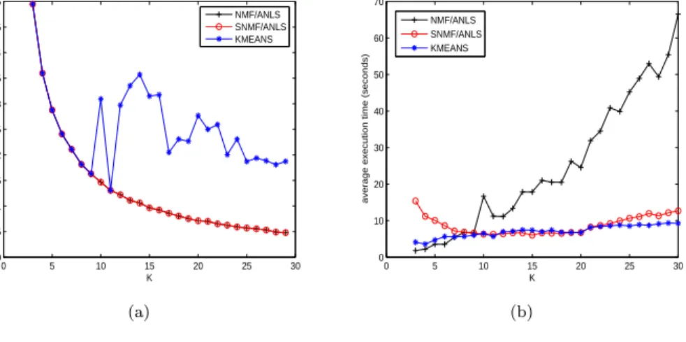
Figure 1: (a) Minimum value of the sum of squared errors and (b) average execution time of 100 trials for various numbers of clusterskon the synthetic data set of 500×1000
0 5 10 15 20 25 30 0 0.5 1 1.5 2 2.5 3 3.5 4 4.5 5x 10 4 K
minimum value of sum of squared error (out of 100 trials)
NMF/ANLS SNMF/ANLS KMEANS (a) 0 5 10 15 20 25 30 0 10 20 30 40 50 60 70 K
average execution time (seconds)
NMF/ANLS SNMF/ANLS KMEANS
(b)
k≤20. Up tok= 30, SNMF continued to give the optimal assignment for some part of our 100 trials. In the case of NMF, we see that a good amount of optimal assignments were found for allk’s up tok= 30.
We also observed how good each method achieved in terms of the sum of squared errors (SSE) objective function. The SSE is defined as Eq. (3), i.e.,Pk
j=1
P
ai∈Cjkai−cjk
2
where cj is the centroid of cluster
Cj. The minimum values of the SSE from 100 trials are presented in Fig. 1-(a). The graphs of NMF and
SNMF represent in fact the value of the optimal assignment since both NMF algorithms achieved at least one optimal assignment across allk’s. The graph of K-means shows that the assignment obtained by K-means was far from the optimal assignment.
In order to compare the time complexity, the average execution time is summarized in Fig. 1-(b). In general, the execution time required for SNMF and K-means were comparable across variouskvalues. When k≤7, SNMF took more time than K-means, but this is not much of a problem in practice considering that SNMF produced the optimal assignments in all 100 trials. The increasing trend of execution time of NMF was because that NMF required more iterations of ANLS than SNMF. In SNMF, askincreases, theH factor became more sparse and the algorithm finished with less iterations of ANLS.
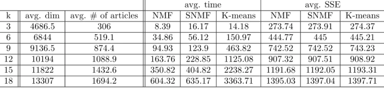
Table 2: Data set information and execution results about the experiment using TDT2 text corpus. For various numbers of clusterk, 10 sets ofktopics were randomly chosen where each topic has between 30 and 300 articles. Average dimension and number of articles across the 10 sets are shown in the left half. Average execution time and the sum of squared errors are shown in the right half.
avg. time avg. SSE
k avg. dim avg. # of articles NMF SNMF K-means NMF SNMF K-means 3 4686.5 306 8.39 16.17 14.18 273.74 273.91 274.37 6 6844 519.1 34.86 56.12 150.97 444.77 445 445.21 9 9136.5 874.4 94.93 123.9 463.82 742.52 742.52 743.23 12 10194 1088.9 163.76 228.85 1125.08 907.32 907.51 908.92 15 11822 1432.6 350.82 404.82 2238.27 1191.68 1192.05 1193.31 18 13307 1694.2 604.32 635.17 3363.71 1395.03 1397.04 1397.71
4.3
Results on Text Data Sets
In this section, we present test results performed on Topic Detection and Tracking 2 (TDT2) text corpus1.
The data set TDT2 contains news articles from various sources such as NYT, CNN, VOA, etc. in 1998. The corpus was manually labeled across 100 different topics, and it has been widely used for the evaluation of text classification or clustering.
We constructed our test data from the TDT2 corpus in the following way. In TDT2 corpus, The topic assignment of each article is labeled either ‘YES’ or ‘BRIEF’ indicating whether the article is definitely or loosely related to the topic. We used only the articles with label ‘YES’ for clear separation of topics. The number of articles in each category is very unbalanced ranging from 1 to 1440. Since too unbalanced categories might mislead the performance test, only categories with the number of data items between 30 and 300 were used. As a result, we had 36 categories with the number of articles from 30 to 278. From this, we randomly chose 10 sets ofk categories for each k= 3,6,9,12,15,18. Average dimension and size for constructed data set is shown in Table. 2. The term-document matrix was created by TF.IDF indexing and unit-norm normalization [10].
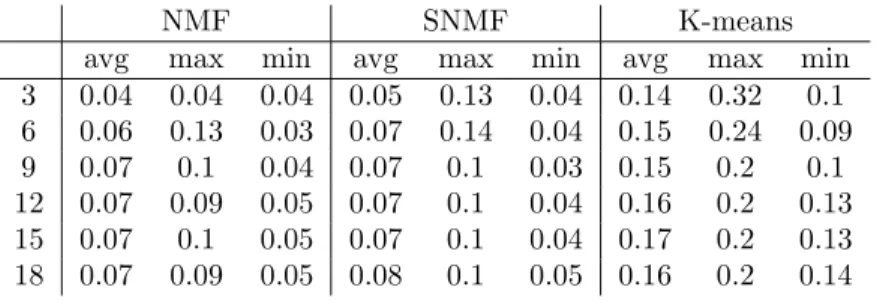
Tables 3 and 4 present the results from this data set. We conducted 10 random trials with each method in order to compare the best performance and consistency. From the 10 random trials, we obtained minimum, maximum, and average value of purity and entropy. Then the values are again averaged over the 10 different data sets of size k. As shown in Table 3 and 4, NMF and SNMF outperformed K-means in both purity and entropy measures. The best performances of algorithms are found from maximum values of purity and minimum values of entropy, where NMF and SNMF consistently outperformed K-means. In general, we observe that the difference between K-means and NMFs becomes larger whenk increases.
We say that a clustering algorithm is consistent if it produces good clustering results under various random initializations. In our experiment, the consistency of each algorithm is evident from the worst results of each algorithm; that is, the minimum value of purity and the maximum value of entropy. The results in Table 3 and 4 imply that NMF and SNMF are consistent even with largek’s. In particular, when kis larger than 12, the minimum purity value of NMF and SNMF is greater than the maximum value of K-means.
Time complexity and the sum of squared errors (SSE) value are shown in Table. 2. Askbecomes larger, the data dimension and size grows correspondingly, and K-means takes a longer time than NMF and SNMF. Average values of sum of squared errors are comparable among all three methods in this case.
4.4
Selection of Parameters in Sparse NMF Algorithm
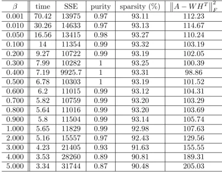
In sparse NMF, the parameterβ was used to control the degree of sparsity. The general behavior of SNMF was not very sensitive toβ, but choosing an appropriate value is still important. The detailed experimental
Table 3: Purity values evaluated from the results on the text data set from TDT2 corpus. Average, minimum, and maximum values out of 10 trials are shown.
NMF SNMF K-means
avg max min avg max min avg max min 3 0.99 0.99 0.99 0.98 0.99 0.93 0.95 0.98 0.83 6 0.96 0.99 0.9 0.95 0.98 0.9 0.89 0.96 0.82 9 0.95 0.97 0.92 0.95 0.98 0.92 0.88 0.93 0.81 12 0.94 0.97 0.92 0.94 0.98 0.91 0.86 0.9 0.8 15 0.94 0.96 0.91 0.93 0.96 0.9 0.83 0.88 0.79 18 0.94 0.96 0.91 0.93 0.96 0.9 0.83 0.86 0.78
Table 4: Entropy values evaluated from the results on the text data set from TDT2 corpus. Average, minimum, and maximum values out of 10 trials are shown.
NMF SNMF K-means
avg max min avg max min avg max min 3 0.04 0.04 0.04 0.05 0.13 0.04 0.14 0.32 0.1 6 0.06 0.13 0.03 0.07 0.14 0.04 0.15 0.24 0.09 9 0.07 0.1 0.04 0.07 0.1 0.03 0.15 0.2 0.1 12 0.07 0.09 0.05 0.07 0.1 0.04 0.16 0.2 0.13 15 0.07 0.1 0.05 0.07 0.1 0.04 0.17 0.2 0.13 18 0.07 0.09 0.05 0.08 0.1 0.05 0.16 0.2 0.14
results are provided in Tables 8 and 9. Table 8 shows performance evaluations on a synthetic data set with variousβ values, and Table 9 shows the results from a text data set with variousβ values. For the synthetic data set (Table 8),β values from 0.3 to 0.5 showed good performance, and for the text data set (Table 9),β values from 0.05 to 0.1 showed good performance. Too bigβ values are not desirable since that might lead to worse approximation. β values around 0.1 are recommended for high dimensional (several thousands or more) and sparse data sets such as the text data used in our experiments. For the experiments in this paper, we usedβ= 0.5 for synthetic data set andβ = 0.1 for text data set.
5
Determination of the Correct Number of Clusters
In most clustering algorithms, the number of clusters to find has to be given as an input. A mechanism by which the correct number of clusters can be determined within the capability of a clustering algorithm can be very useful. In this section, we revisit the model selection method designed to determine the number of clusters in the data set due to Brunet et al. [4] and examine its applicability to the algorithms such as K-means, NMF, and SNMF. We emphasize that the consistency of the clustering algorithm with respect to random initializations is critical in succssful application of this model selection method which SNMF seems to demonstrate.
In order to measure the consistency, a connectivity matrix is defined as follows. The connectivity matrix Ck ∈Rn×n forndata points is constructed from each execution of a clustering algorithm. For each pair of
data pointsiand j, we assignCk(i, j) = 1 if theiand j are assigned to the same cluster, andCk(i, j) = 0
otherwise wherek is the cluster number given as an input to the clustering algorithm. Then the average connectivity matrix ˆCk is computed by averaging the connectivity matrices over trials. The value ˆCk(i, j)
indicates the possibility of two data pointsiandj being assigned to the same cluster, and each element of ˆ
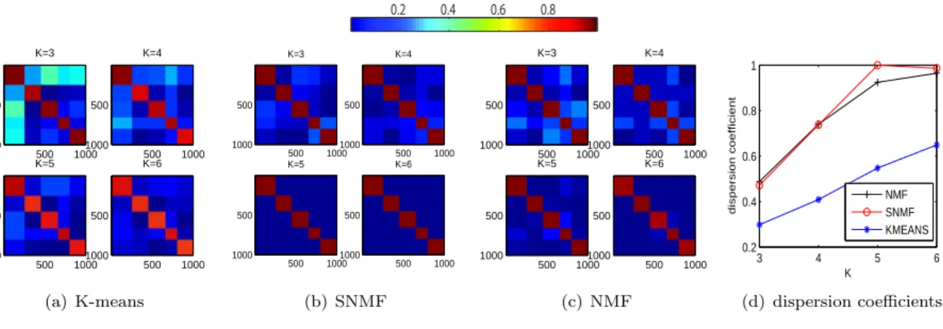
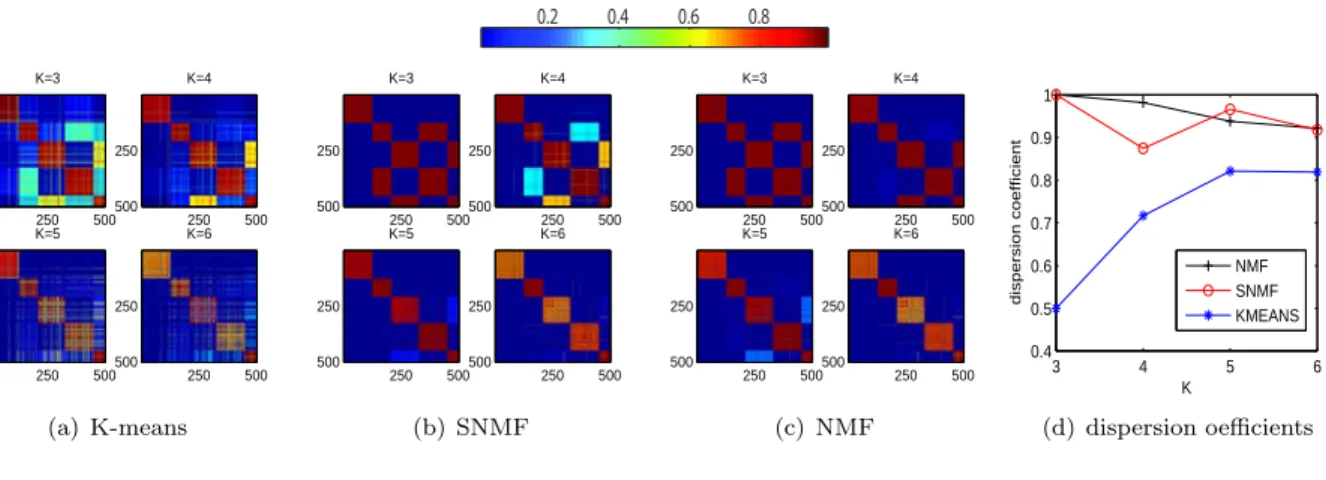
Figure 2: Model selection process for synthetic data set with k = 5. Consensus matrices for several trial values ofk= 3,4,5,6 are shown for each method in (a), (b), and (c). The dispersion coefficients in (d) shows that we could tell the correct number of cluster is 5 from the point where the line of SNMF drops, but the graph from NMF or K-means provide no information to decide the number of cluster.
0.2 0.4 0.6 0.8 K=3 500 1000 500 1000 K=4 500 1000 500 1000 K=5 500 1000 500 1000 K=6 500 1000 500 1000 (a) K-means K=3 500 1000 500 1000 K=4 500 1000 500 1000 K=5 500 1000 500 1000 K=6 500 1000 500 1000 (b) SNMF K=3 500 1000 500 1000 K=4 500 1000 500 1000 K=5 500 1000 500 1000 K=6 500 1000 500 1000 (c) NMF 3 4 5 6 0.2 0.4 0.6 0.8 1 K dispersion coefficient NMF SNMF KMEANS (d) dispersion coefficients ˆ
Ck should be close to either 0 or 1. The general quality of the consistency is summarized by the dispersion
coefficient defined as ρk = 1 n2 n X i=1 n X j=1 4( ˆCk(i, j)− 1 2) 2 (17)
where 0≤ρk ≤1, andρk = 1 represents the perfectly consistent assignment. After obtaining the values of
ρk for variousk’s, the number of clusters could be determined by the pointkwhereρkdrops. The reasoning
behind this rule is as follows. When the number of clustersk used in a clustering algorithm is smaller than true number of clusters, then the clustering assignment may or may not be consistent depending on whether the data set can be partitioned into a smaller number of hyper groups. When the guessed number of clusters k is correct, the clustering assignment should be consistent througout trials assuming that the algorithm is finding the optimal clustering assignment each time. When the guessed number of clustersk is larger than the correct number, it is expected that the clustering assignment is inconsistent. Brunet et al. [4] and Kim and Park [13] successfully used this method to determine the unknown number of groups from gene expression data.
Our study and experimental results explain why this method works for SNMF but does not work for K-means. From Table 1 and Fig. 1, we showed that SNMF finds the optimal assignment of our synthetic data set very consistently. In particular, when k ≤ 12, the solutions of SNMF were always the optimal assignment. This consistency implies that the clustering assignments from SNMF remain the same over repeated trials. In contrast, the assignments of K-means show much less possibility of obtaining the optimal assignment and less consistency. Even for smallkvalues such as 3,4, or 5, K-means only achieved the optimal assignment in less than 50 percent of the trials. When we do not have prior knowledge about the number of clusters, it is difficult to ascertain the correct number of clusters from the K-means results. Thus, the consistency of SNMF is the key factor that enables the model selection method described above.
We demonstrate the process of this model selection method for our synthetic data set with k = 5 in Fig. 2. The consensus matrix is sorted with the true label for a better visual representation. As shown in Fig. 2-(a), (b), and (c), the SNMF showed very clear assignment for the correct number ofkwhile K-means and NMF did not give clear results. The dispersion coefficient is plotted in Fig. 2-(d). From the line of SNMF, one could determine the correct number of clusters from the point whereρk drops, which is 5. The
dispersion coefficient values for NMF and K-means keep increasing withk and the number of clusters can not be determined.
Table 5: Topic description of a text data set for which model selection process is demonstrated in Fig. 3 topic id description number of articles
12 Pope visits Cuba 151 26 Oprah Lawsuit 70 32 Sgt. Gene McKinney 126 48 Jonesboro shooting 125
87 NBA finals 79
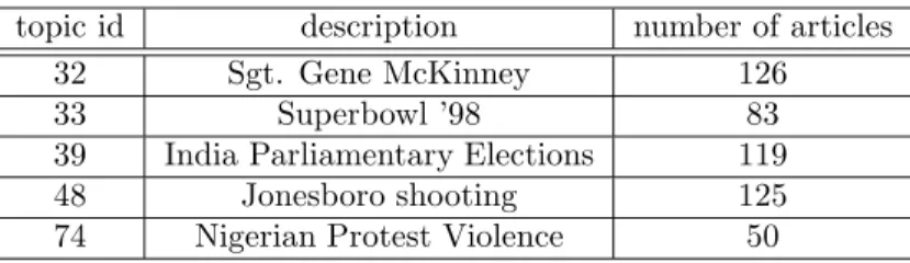
Table 6: Topic description of a text data set for which model selection process is demonstrated in Fig. 4 topic id description number of articles
32 Sgt. Gene McKinney 126
33 Superbowl ’98 83
39 India Parliamentary Elections 119 48 Jonesboro shooting 125 74 Nigerian Protest Violence 50
sets with k = 5. The data sets were constructed by the same method of Sec. 4.3, and their topics are summarized in Tables 5 and 6. For the data set in Table 5, the model selection process is shown in Fig. 3. Similar to the results from the synthetic data set, the consensus matrix of K-means shows that the clustering assignment is inconsistent. The trend of dispersion coefficients of NMF or SNMF (Fig. 3-(d)) shows that the most likely number of clusters is 5. For the second data set in Table 6, Fig. 6 shows the model selection process. From the dispersion coefficients obtained in SNMF, it is suggested that the possible numbers of clusters are 3 or 5 where the largest one is 5. Again, we could correctly determine the correct number of clusters using SNMF.
6
Comparison with Affinity Propagation
Affinity Propagation (AP) was recently proposed by Frey and Dueck [8]. The objective function in AP is the same as K-means clustering shown in Eq. (3). Since this new method is claimed to efficiently minimize the objective function, we tested AP on our data set and compared the results with those from NMFs. A short description of the AP algorithm and experimental results follow.
One of the key differences between AP and other clustering methods is that it does not take the target number of clusters as an input parameter. Instead, it determines the number of clusters from the data and other input parameters. There are two groups of input parameters of AP: similarities and self preferences. The similarities are defined for two distinct data pointsiandj, and the values(i, k) represents how much the pointkcould explain the pointi. The similarity values do not need to be symmetric; that is,s(i, k)6=s(k, i) in general. When AP is formed to minimize the sum of squared errors objective function, the similarity values are set to be the negative squared distances; s(i, k) = s(k, i) = − kxi−xkk2 where xi and xk are
vectors that represent data pointsiandk.
The second group of parameters is called self preferences, which is defined for each data point. The preference of data pointi, which is written ass(i, i), shows the degree of confidence that the pointishould be a cluster exemplar. Preference values could be set differently for each data pointi, especially if relevant prior information is available. A common assumption is that every data point has equal possibility of being a cluster exemplar, and therefore preference values are set to a constant across all data points. The number of clusters returned by the AP algorithm depends upon this parameter. When preference value becomes
Figure 3: Model selection process for the text data set in Table 5. Consensus matrices for several trial values ofk= 3,4,5,6 are shown for each method in (a), (b), and (c). The dispersion coefficients in (d) shows that we could tell the correct number of cluster is 5 from the point where the graph of SNMF drops. The graph of NMF provides the same information, but we can not say the number of clusters from the graph of K-means.
0.2 0.4 0.6 0.8 K=3 250 500 250 500 K=4 250 500 250 500 K=5 250 500 250 500 K=6 250 500 250 500 (a) K-means K=3 250 500 250 500 K=4 250 500 250 500 K=5 250 500 250 500 K=6 250 500 250 500 (b) SNMF K=3 250 500 250 500 K=4 250 500 250 500 K=5 250 500 250 500 K=6 250 500 250 500 (c) NMF 3 4 5 6 0.4 0.5 0.6 0.7 0.8 0.9 1 K dispersion coefficient NMF SNMF KMEANS (d) dispersion coefficients
larger, the number of clusters returned by AP is also larger; when preference value becomes smaller, we have smaller number of clusters from the AP algorithm. Recommended value of the preference is the median of similarity values.
Given these input values, AP alternates two kinds of message passing between data points until conver-gence. The responsibility messager(i, k), which is sent from data pointitok, shows the dynamic degree of possibility that the data pointkcould be an exemplar ofi. The availability messagea(i, k), which is sent from data point k to i, contains the dynamic degree of confidence for how good if the data point i could choose pointkas its exemplar. The two messages are updated until convergence by the following rules.
1. updater(i, k) by
s(i, k)−maxk′s.t. k′6=k{a(i, k′) +s(i, k′)}
2. updatea(i, k) by minn0, r(k, k) +P
i′s.t. i′∈{/ i,k}max{0, r(i′, k)}
o
ifi6=k 3. updatea(k, k) by
P
i′s.t. i′6=kmax{0, r(i′, k)}
In order to avoid oscillations, an additional parameterλ, which is called damping factor, is introduced so that each message is updated by a linear combination of the value at the previous step and the value newly computed. Overall, the results of AP only depends on input parameters and data; hence, one does not need to run AP several times. Instead, there are input paramters, especially the preference values, where appropriate values need to be decided.
We used the AP implementation provided by the authors [8] with default configurations. For our syn-thetic data set, AP showed good performance. Across all valuesk= 3,4,· · ·,30, AP obtained the optimal assignments using the default strategy for preference values, i.e., the median of similarities. With respect to the time complexity, AP used 23.45 seconds for each run while SNMF took 8.69 seconds on average for each run. Although SNMF required less time for each run, one might want to run SNMF several times to obtain the best solution; thus, one cannot directly compare the execution time of the two algorithms.
For the text data set, the median of similarities as the preference value did not work well. For example, for a text data set with 6 clusters, AP with median of similarities as preference returned 72 as an estimated number of clusters. For another text data set with 15 clusters, AP with median strategy estimated 167
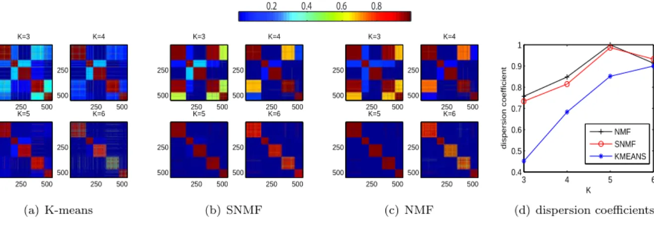
Figure 4: Model selection process for the text data set in Table 6. Consensus matrices for several trial values ofk= 3,4,5,6 are shown for each method in (a), (b), and (c). The dispersion coefficients of SNMF in (d) indicates that clustering assignments are consistent fork = 3,5 but not consistent for k = 4,6 suggesting that the possible numbers of clusters are 3 or 5 where the largest number is 5. The graph from NMF or K-means provide no information to decide the number of clusters.
0.2 0.4 0.6 0.8 K=3 250 500 250 500 K=4 250 500 250 500 K=5 250 500 250 500 K=6 250 500 250 500 (a) K-means K=3 250 500 250 500 K=4 250 500 250 500 K=5 250 500 250 500 K=6 250 500 250 500 (b) SNMF K=3 250 500 250 500 K=4 250 500 250 500 K=5 250 500 250 500 K=6 250 500 250 500 (c) NMF 3 4 5 6 0.4 0.5 0.6 0.7 0.8 0.9 1 K dispersion coefficient NMF SNMF KMEANS (d) dispersion oefficients
clusters. In order to mitigate this situation, we used the following naive search strategy. When we want to observe the result of AP on a data set where number of clusters is known, we first try the median of similarities as a tentative value of preference and decide a step size by which the preference value will be updated. If the estimated number of clusters is smaller (greater) than the correct number, then increase (decrease) the preference value by an amount of the step size until the returned value becomes equal to or greater (smaller) than the correct number. If the correct number is not achieved, we start a binary search until the correct number is obtained. After some trials and errors, we initialized the step size by taking the difference of maximum and minimum similarity values and multiplying by 3.
Execution results on text data set are shown in Table 7. In general, the measures were good and comparable to the result of SNMF in Tables 2, 3, and 4. Average purity and entropy values were about the same, but the best values of purity and entropy of SNMF were better than that of AP. Average execution time of AP was shorter than that of SNMF.
In summary, AP and SNMF showed comparable average performance. While AP had advantage in execution time, SNMF had advantage in the quality of best solutions. In addition, SNMF has another benefit. AP is claimed to automatically catch the number of clusters from data, but the number of clusters depends upon the preference parameter. Our experiments assumed the number of clusters is known; however, when the number of clusters is unknown, AP does not provide a measure to determine correct number of clusters. In the sections above, we demonstrated that SNMF gives consistent solutions, thus the model selection by consensus matrix could be applied.
7
Conclusion
In this paper, we studied the properties of NMF as a clustering method by relating its formulation to K-means clustering. We presented the objective function of K-means as a lower rank approximation and observed that some constraints can be relaxed from K-means to achieve NMF formulation. Sparsity constraints were imposed on the coefficient matrix factor in order to mitigate this relaxation. Experimental results show that sparse NMF gives very good and consistent solutions to the clustering problem. The consistency enables a model selection method based on the consensus matrix. Compared to the recently proposed Affinity Propagation algorithm, sparse NMF showed comparable results.
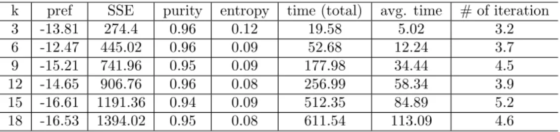
Table 7: Execution results of Affinity Propagation for TDT2 text data set of Table 2. The ‘pref’ column shows the preference value where the desired number of cluster is achieved. The ‘iteration’ column shows how many times we need to run AP to find the desired number of clusters based on our simple strategy. The ‘time (total)’ column shows the total time used to find the result with desired number of clusters, and the ‘avg. time’ column shows the average execution time of each AP run.
k pref SSE purity entropy time (total) avg. time # of iteration 3 -13.81 274.4 0.96 0.12 19.58 5.02 3.2 6 -12.47 445.02 0.96 0.09 52.68 12.24 3.7 9 -15.21 741.96 0.95 0.09 177.98 34.44 4.5 12 -14.65 906.76 0.96 0.08 256.99 58.34 3.9 15 -16.61 1191.36 0.94 0.09 512.35 84.89 5.2 18 -16.53 1394.02 0.95 0.08 611.54 113.09 4.6
as a clustering method. LettingG=BD−1
2, we have h(G) = min G≥0 A−AGGT 2 F (18)
where G ∈Rn×k has exactly one positive element for each row. The condition on G can be replaced by {G≥ 0 and GTG=I}, and we could determine the cluster membership of each data point based on the largest elements in each row of G. Currently, we are exploring the behavior of the following NMF as an alternative clustering method and developing a new algorithm based on this formulation:
G= arg min G≥0,GTG=I A−AGGT . (19)
References
[1] M. H. V. Benthem and M. R. Keenan. Fast algorithm for the solution of large-scale non-negativity-constrained least squares problems. Journal of Chemometrics, 18:441–450, 2004.
[2] P. S. Bradley and U. M. Fayyad. Refining initial points for k-means clustering. In Proceedings of the Fifteenth International Conference on Machine Learning, pages 91–99. Morgan Kaufmann Publishers Inc. San Francisco, CA, USA, 1998.
[3] R. Bro and S. D. Jong. A fast non-negativity-constrained least squares algorithm. Journal of Chemo-metrics, 11:393–401, 1997.
[4] J. Brunet, P. Tamayo, T. Golub, and J. Mesirov. Metagenes and molecular pattern discovery using matrix factorization. Proceedings of the National Academy of Sciences, 101(12):4164–4169, 2004. [5] I. S. Dhillon, Y. Guan, and J. Kogan. Refining clusters in high-dimensional text data. In
Proceed-ings of the Workshop on Clustering High Dimensional Data and its Applications at the Second SIAM International Conference on Data Mining, pages 71–82, 2002.
[6] C. Ding, X. He, and H. D. Simon. On the equivalence of nonnegative matrix factorization and spectral clustering. InProceedings of SIAM Internationall Conference on Data Mining, 2005.
[7] D. Donoho and V. Stodden. When does non-negative matrix factorization give a correct decomposition into parts? In S. Thrun, L. Saul, and B. Sch¨olkopf, editors,Advances in Neural Information Processing Systems 16. MIT Press, Cambridge, MA, 2004.
Table 8: Performance evaluation for various β values with the synthetic data set, k = 15. The degree of sparsity is shown as the average percentage of number of zero elements in the factorH.
β time SSE purity sparsity (%)
A−W HT 2 F 0.001 70.42 13975 0.97 93.11 112.23 0.010 30.26 14633 0.97 93.13 114.67 0.050 16.56 13415 0.98 93.27 110.24 0.100 14 11354 0.99 93.32 103.19 0.200 9.27 10722 0.99 93.19 102.05 0.300 7.99 10282 1 93.25 100.39 0.400 7.19 9925.7 1 93.31 98.86 0.500 6.78 10303 1 93.19 101.52 0.600 6.2 11015 0.99 93.12 104.31 0.700 5.82 10759 0.99 93.20 103.29 0.800 5.64 11016 0.99 93.20 103.69 0.900 5.8 11504 0.99 93.14 105.74 1.000 5.65 11829 0.99 92.98 107.63 2.000 5.16 15557 0.97 92.43 129.56 3.000 4.23 21405 0.93 91.63 155.55 4.000 3.53 28260 0.89 90.81 189.31 5.000 3.34 31744 0.87 90.48 205.03
Table 9: Performance evaluation for variousβ values with TDT2 text data set,k= 9. The degree of sparsity is shown as the average percentage of number of zero elements in the factorH.
β time SSE purity sparsity (%)
A−W HT 2 F 0.001 363.9 742.26 0.95 53.25 26.84 0.010 203.27 742.47 0.95 63.79 26.85 0.050 142.72 742.21 0.95 74.25 26.86 0.100 132.77 742.42 0.95 78.32 26.87 0.200 133.89 742.93 0.95 81.66 26.9 0.300 126.02 743.15 0.94 83.14 26.92 0.400 130.58 743.52 0.94 84.20 26.95 0.500 141.78 744.13 0.94 84.82 26.97 0.600 142.75 743.52 0.94 85.45 26.98 0.700 130.15 745.64 0.93 85.75 27.03 0.800 129.23 746.2 0.93 86.08 27.06 0.900 116.12 747.15 0.93 86.18 27.09 1.000 138.5 746.21 0.93 86.42 27.09 2.000 52.89 769.73 0.78 86.13 27.83 3.000 30.11 784.87 0.68 86.54 28.45 4.000 26.35 791.13 0.63 87.28 28.8 5.000 25.61 795.87 0.61 87.83 29.01
[8] B. J. Frey and D. Dueck. Clustering by passing messages between data points. Science, 315:972–976, 2007.
[9] G. Golub and C. Van Loan. Matrix computations. Johns Hopkins University Press Baltimore, MD, USA, 1996.
[10] D. A. Grossman and O. Frieder. Information Retrieval: Algorithms And Heuristics. Springer, 2004. [11] P. O. Hoyer. Non-negative matrix factorization with sparseness constraints. The Journal of Machine
Learning Research, 5:1457–1469, 2004.
[12] H. Kim and H. Park. Non-negative matrix factorization based on alternating non-negativity constrained least squares and active set method. Technical report, Technical Report GT-CSE-07-01, College of Computing, Georgia Institute of Technology, 2007.
[13] H. Kim and H. Park. Sparse non-negative matrix factorizations via alternating non-negativity-constrained least squares for microarray data analysis. Bioinformatics, 23(12):1495–1502, 2007. [14] D. Lee and H. Seung. Learning the parts of objects by non-negative matrix factorization. Nature,
401(6755):788–791, 1999.
[15] S. Z. Li, X. Hou, H. Zhang, and Q. Cheng. Learning spatially localized, parts-based representation. In CVPR ’01: Proceedings of the 2001 IEEE Computer Society Conference on Computer Vision and Pattern Recognition, volume 1, 2001.
[16] P. Paatero and U. Tapper. Positive matrix factorization: A non-negative factor model with optimal utilization of error estimates of data values. Environmetrics, 5(1):111–126, 1994.
[17] F. Shahnaz, M. Berry, V. Pauca, and R. Plemmons. Document clustering using nonnegative matrix factorization. Information Processing and Management, 42(2):373–386, 2006.
[18] R. Tibshirani. Regression shrinkage and selection via the lasso.Journal of the Royal Statistical Society. Series B (Methodological), 58(1):267–288, 1996.
[19] W. Xu, X. Liu, and Y. Gong. Document clustering based on non-negative matrix factorization. InSIGIR ’03: Proceedings of the 26th annual international ACM SIGIR conference on Research and development in informaion retrieval, pages 267–273, New York, NY, USA, 2003. ACM Press.
[20] H. Zha, C. Ding, M. Gu, X. He, and H. Simon. Spectral relaxation for k-means clustering. InAdvances in Neural Information Processing Systems, volume 14, pages 1057–1064. MIT Press, 2002.