for fraud detection in mobile
communications networks
Jaakko Hollm´en
Helsinki University of Technology
Department of Computer Science and Engineering Laboratory of Computer and Information Science
Dissertation for the degree of Doctor of Science in Technology to be pre-sented with due permission of the Department of Computer Science and En-gineering, for public examination and debate in Auditorium T2 at Helsinki University of Technology (Espoo, Finland) on the 19th of December, 2000, at 12 noon.
Hollm´en, J.,User profiling and classification for fraud detection in mobile communications networks. ISBN 951-22-5239-2. (also pub-lished in print ISBN 951-666-555-1, ISSN 1456-9418). viii + 47 pp. UDC 004.032.26:519.21:621.391.
Keywords: fraud detection, telecommunication, neural networks, probabilis-tic models, data analysis, data mining.
ABSTRACT
The topic of this thesis is fraud detection in mobile communications net-works by means of user profiling and classification techniques. The goal is to first identify relevant user groups based on call data and then to assign a user to a relevant group. Fraud may be defined as a dishonest or illegal use of services, with the intention to avoid service charges. Fraud detection is an important application, since networkoperators lose a relevant portion of their revenue to fraud. Whereas the intentions of the mobile phone users cannot be observed, it is assumed that the intentions are reflected in the call data. The call data is subsequently used in describing behavioral patterns of users. Neural networks and probabilistic models are employed in learn-ing these usage patterns from call data. These models are used either to detect abrupt changes in established usage patterns or to recognize typical usage patterns of fraud. The methods are shown to be effective in detecting fraudulent behavior by empirically testing the methods with data from real mobile communications networks.
© All rights reserved. No part of this publication may be reproduced, stored in a retrieval system, or transmitted, in any form or by any means, electronic, mechanical, photocopying, recording, or otherwise, without the prior permission of the author.
The workpresented in this thesis was carried out at the Laboratory of Com-puter and Information Science in the Department of ComCom-puter Science and Engineering of the Helsinki University of Technology and Siemens Corporate Technology, Information and Communications, Department of Neural Com-putation in Munich, Germany. Funding was received from both institutions. Additional financial support was received from the Finnish Foundation for the Promotion of Technology, the Emil Aaltonen Foundation, and the NEu-roNet — the European Networkof Excellence in neural networks, set up under European Commission’s ESPRIT III Program. A travel grant was received from the NIPS Foundation.
I wish to thankProfessor Olli Simula for supervising my graduate studies and for guidance and encouragement during the thesis work. The Depart-ment of Neural Computation at Siemens Corporate Technology, headed by Professor Bernd Sch¨urmann, provided an interesting subject for research. I would like to thank Michiaki Taniguchi and Volker Tresp, who lead the research groups I worked with at Siemens. I am especially indebted to Volker Tresp for guiding my research and for introducing me to probabilis-tic modeling. I also wish to thankmy co-authors and colleagues for their collaboration. Academy Professor Erkki Oja and Academician Teuvo Ko-honen have influenced this workthrough their pioneering work, also the Laboratory of Computer and Information Science and the Neural Networks Research Centre provided excellent facilities for research under their man-agement. I wish to thankProfessors Henry Tirri and Jyrki Joutsensalo for reviewing the manuscript of the thesis. I thankDocent Aapo Hyv¨arinen and Professor MarkGirolami for comments on the work. Finally, without the support and encouragement of my family, Suvi and Risto, this thesis work would not have been possible.
Abstract . . . ii
Preface . . . iii
List of publications . . . vi
Abbreviations and notations. . . viii
1 Introduction . . . 1
2 Fraud detection . . . 3
2.1 Introduction . . . 3
2.1.1 Definition of fraud . . . 3
2.1.2 Motivation for fraud detection . . . 3
2.1.3 Development of fraud . . . 4
2.2 Previous work . . . 5
2.2.1 Comparisons of the published work. . . 8
2.3 Related areas . . . 8
2.3.1 Intrusion detection on computer systems . . . 8
2.3.2 Credit card fraud detection . . . 9
2.3.3 Other work on fraud detection . . . 10
2.4 Discussion . . . 10
3 Call data . . . 12
3.1 Data Collection . . . 12
3.1.1 Block crediting . . . 13
3.1.2 Velocity trap . . . 13
3.2 Representation of call data . . . 14
3.2.1 Features through aggregation in time . . . 14
3.2.2 Dynamic description of call data . . . 15
3.2.3 Switching representation . . . 15
4 User profiling and classification . . . 16
4.1 Probabilistic networks . . . 16
4.1.1 Conditional independence . . . 17
4.1.2 Distributional assumptions . . . 18
4.1.3 Learning by EM algorithm . . . 18 iv
4.1.4 Finite mixture models . . . 20
4.1.5 Hidden Mark ov models (HMM) . . . 20
4.1.6 Hierarchical regime-switching model . . . 22
4.2 Self-Organizing Map (SOM) . . . 23
4.2.1 SOM algorithm . . . 23
4.2.2 SOM in process monitoring . . . 24
4.2.3 SOM for clustering probabilistic models . . . 25
4.3 Learning Vector Quantization (LVQ) . . . 26
4.3.1 LVQ algorithm . . . 26
4.3.2 LVQ for probabilistic models . . . 26
4.4 Cost-sensitive classification . . . 27
4.4.1 Input-dependent misclassification cost . . . 27
4.5 Assessment of models . . . 28
4.5.1 Assessment of diagnostic accuracy . . . 28
4.5.2 Cost assessment . . . 30
4.5.3 Relationship between ROC analysis and cost . . . 30
4.6 Discussion . . . 31
5 Conclusions . . . 32
5.1 Summary . . . 32
5.2 Further work . . . 33
6 Publications . . . 35
6.1 Contents of the publications . . . 35
6.2 Contributions of the author . . . 37
6.3 Errata . . . 37
References . . . 38
This thesis consists of an introduction and the following publications:
Publication 1: Alhoniemi, E., J. Hollm´en, O. Simula, and J. Vesanto (1999). Process monitoring and modeling using the self-organi-zing map. Integrated Computer Aided Engineering 6(1), 3–14.
Publication 2: Taniguchi, M., M. Haft, J. Hollm´en, and V. Tresp (1998). Fraud detection in communication networks using neu-ral and probabilistic methods. InProceedings of the 1998 IEEE International Conference in Acoustics, Speech and Signal Pro-cessing (ICASSP’98), Volume II, pp. 1241–1244.
Publication 3: Hollm´en, J. and V. Tresp (1999). Call-based fraud de-tection in mobile communication networks using a hierarchical regime-switching model. In M. Kearns, S. Solla, and D. Cohn (Eds.), Advances in Neural Information Processing Systems 11: Proceedings of the 1998 Conference (NIPS’11), pp. 889–895. MIT Press.
Publication 4: Hollm´en, J., V. Tresp, and O. Simula (1999). A self-organizing map for clustering probabilistic models. In Proceed-ings of the Ninth International Conference on Artificial Neural Networks (ICANN’99), Volume 2, pp. 946–951. IEE.
Publication 5: Hollm´en, J., M. Skubacz, and M. Taniguchi (2000). Input dependent misclassification costs for cost-sensitive classifi-cation. In N. Ebecken and C. Brebbia (Eds.),DATA MINING II — Proceedings of the Second International Conference on Data Mining 2000, pp. 495–503. WIT Press.
Publication 6: Hollm´en, J. and V. Tresp (2000). A hidden markov model for metric and event-based data. In Proceedings of EU-SIPCO 2000 — X European Signal Processing Conference, Vol-ume II, pp. 737–740.
Publication 7: Hollm´en, J., V. Tresp, and O. Simula (2000). A learn-ing vector quantization algorithm for probabilistic models. In
Proceedings of EUSIPCO 2000 — X European Signal Processing Conference, Volume II, pp. 721–724.
BMU Best-Matching Unit (also winner unit) DAG Directed Acyclic Graph
EM Expectation Maximization algorithm GSM Global System for Mobile communications
HMM Hidden Markov Model
KL Kullback-Leibler distance LVQ Learning Vector Quantization
ROC Receiver Operating Characteristic curve SOM Self-Organizing Map
α(t) adaptation gain value, also learning rate c index of the winner unit
δ(x−xi) unit impulse function atxi ∂/∂x partial derivative with regard tox
i, k unit index
hc(t, k) neighborhood kernel function λij cost of classifyingj asi
λij(x) cost of classifyingj asi parameterized by data mi(t), mi weight vector of the uniti
P(S) probability of hidden state vectors1, . . . , sT
P(st) probability of a hidden variablesat timet P(st|st−1) conditional probability ofst givenst−1
p(x) probability density ofx
q(x; θ) probability density ofx(parameterized byθ) rk, rc location vector inside the array of neurons R(αi|x) conditional riskof classifyingxto the classi σ(t) neighborhood kernel width function
x(t), xi measurement vector
x∼p(x) xis distributed according top(x) Y observed variabley1, . . . , yT yt observed variabley at time t
. Euclidean distance
Introduction
The topic of this thesis is fraud detection in mobile communications networks by means of user profiling and classification techniques. User profiling is the process of modeling characteristic aspects of user behavior. In user classification, users are assigned to distinctive groups.
Fraud may be defined as a dishonest or illegal use of services, with the in-tention to avoid service charges. With the aid of the fraud detection models, fraudulent activity in a mobile communications networkmay be revealed. This is beneficial to the networkoperator, who may lose several percent of revenue to fraud, since the service charges from the fraudulent activity remain uncollected. Apart from fraud detection, user profiling efforts in telecommunications may be further motivated by the need to understand the behavior of customers to enable provision of matching services and to improve operations.
Fraud is defined through the unobserved intentions of the mobile phone users. However, the intentions are reflected in the observed call data, which is subsequently used in describing behavioral patterns of users. The taskis to use the call data to learn models of calling behavior so that these models make inferences about users’ intentions. Neural networks and probabilistic models are employed in learning these usage patterns from call data. Learn-ing in this context means adaptation of the parameterized models so that the inherent problem structure is coded in the model. Obviously, there is no specific sequence of calls that would be fraudulent with absolute certainty. In fact, the same sequence of calls could as well be fraudulent or normal. Therefore, uncertainty in modeling the problem is needed. This is naturally embodied in the frameworkof probabilistic models.
Two complementary approaches to fraud detection are used in this thesis. In the differential approach, a model of recent behavior is used in quanti-fying novelty found in the future call data so as to detect abrupt changes in the calling behavior, which may be a consequence of fraud. In the abso-lute approach, models typifying fraudulent and normal behavior are used to
determine the most likely mode.
Chapter 2 introduces the problem of fraud detection and presents a re-view of the published works in telecommunications fraud detection. Related fields such as intrusion detection in computer systems and credit card fraud detection are also briefly reviewed. In Chapter 3, the call data used in this thesis is described. Chapter 4 forms the core of this thesis, where the novel developments are put in a broader framework. The chapter starts by introducing probabilistic networks, a framework under which mixture models (Publication 2), regime-switching models (Publication 3), and extensions of hidden Markov models (Publication 6) are described. The chapter continues with the presentation of Self-Organizing Maps, which are applied in a related application in process monitoring (Publication 1) and in clustering probabilistic models (Publication 4). Since detection is in-herently a discrimination problem, discriminative learning on top of the Self-Organizing Map is presented in the context of Learning Vector Quanti-zation (Publication 7). The chapter proceeds by introducing cost models that can be used in expressinguser-specific costs (Publication 5). Chap-ter 4 ends with a description of measuring the quality of the models and related discussion. The workis summarized in Chapter 5. Chapter 6 lists the contents of the publications and contributions of the author.
Fraud detection
This chapter introduces the problem of fraud detection, starting from defi-nitions and proceeding to a review of previous work. The end of the chapter discusses the related workin this area.
2.1
Introduction
In this section, fraud is defined and the development of fraud detection systems is motivated. Some historical background is used to motivate the user profiling approaches in fraud detection.
2.1.1 Definition of fraud
Many definitions in the literature exist, where the intention of the subscriber plays a central role. Johnson (1996) defines fraud as any transmission of voice or data across a telecommunications networkwhere the intent of the sender is to avoid or reduce legitimate call charges. In similar vein, Davis and Goyal (1993) define fraud as obtaining unbillable services and unde-served fees. According to Johnson (1996), the serious fraudster sees himself as an entrepreneur, admittedly utilizing illegal methods, but motivated and directed by essentially the same issues of cost, marketing, pricing, network design and operations as any legitimate networkoperator. Hoath (1998) con-siders fraud as attractive from the fraudsters’ point of view, since detection riskis low, no special equipment is needed, and the product in question is easily converted to cash. Although the term fraud has a particular meaning in legislation, this established term is used broadly to mean misuse, dishon-est intention or improper conduct without implying any legal consequences.
2.1.2 Motivation for fraud detection
Following the definition of fraud, it is easy to state the losses caused by fraud as primary motivation for fraud detection. In fact, the telecommunications
industry suffers losses in the order of billions of US dollars annually due to fraud in its networks (Davis and Goyal 1993; Johnson 1996; Parker 1996; O’Shea 1997; Pequeno 1997; Hoath 1998). In addition to financial losses, fraud may cause distress, loss of service, and loss of customer confidence (Hoath 1998). The financial losses account for about 2 percent to 6 percent of the total revenue of networkoperators, thus playing a significant role in total earnings. However, as noted by Barson et al. (1996), it is difficult to provide precise estimates, since some fraud may be never detected, and the operators are reluctant to reveal figures on fraud losses. Since the operators are facing increasing competition and losses have been on the rise (Parker 1996), fraud has gone from being a problem carriers were willing to tolerate to being one that dominates the front pages of both trade and general press (O’Shea 1997). Johnson (1996) also affirms that networkoperators see call selling as a growing concern.
2.1.3 Development of fraud
Historically, earlier types of fraud used technological means to acquire free access. Cloning of mobile phones by creating copies of mobile terminals with identification numbers from legitimate subscribers was used as a means of gaining free access (Davis and Goyal 1993). In the era of analog mobile terminals, identification numbers could be easily captured by eavesdropping with suitable receiver equipment in public places, where mobile phones were evidently used. One specific type of fraud, tumbling, was quite prevalent in the United States (Davis and Goyal 1993). It exploited deficiencies in the validation of subscriber identity when a mobile phone subscription was used outside of the subscriber’s home area. The fraudster kept tumbling (switching between) captured identification numbers to gain access. Davis and Goyal (1993) state that the tumbling and cloning fraud have been seri-ous threats to operators’ revenues. First fraud detection systems examined whether two instances of one subscription were used at the same time (over-lapping calls detection mechanism) or at locations far apart in temporal proximity (velocity trap). Both the overlapping calls and the velocity trap try to detect the existence of two mobile phones with identical identification codes, clearly evidencing cloning. As a countermeasure to these fraud types, technological improvements were introduced.
However, new forms of fraud came into existence. A few years later, O’Shea (1997) reports the so-called subscription fraud to be the trendi-est and the fasttrendi-est-growing type of fraud. In similar spirit, Hoath (1998) characterizes subscription fraud as being probably the most significant and prevalent worldwide telecommunications fraud type. In subscription fraud, a fraudster obtains a subscription (possibly with false identification) and starts a fraudulent activity with no intention to pay the bill. It is indeed non-technical in nature and by call selling, the entrepreneur-minded
fraud-ster can generate significant revenues for a minimal investment in a very short period of time (Johnson 1996). From the above explanation it is ev-ident that the detection mechanisms of the first generation soon became inadequate. The more advanced detection mechanisms must be based on the behavioral modeling of calling activity, which is also the subject of this thesis.
2.2
Previous work
In this section, published workwith relevance to fraud detection in telecom-munications networks is reviewed. Section 2.3 presents fraud detection meth-ods in related fields, such as intrusion detection in computer systems, credit card fraud detection, and applications in other fields, such as health care fraud detection.
Fraud in telecommunications networks can be characterized by fraud sce-narios, which essentially describe how the fraudster gained the illegitimate access to the network. Detection methodologies designed for one specific scenario are likely to miss plenty of the others. For example, velocity trap and overlapping calls detection methodologies are solely aimed at detecting cloned instances of mobile phones and do not catch any of the subscription fraud cases. As stated in Section 2.1.3, the nature of fraud has changed from cloning fraud to subscription fraud, which makes specialized detection methodologies inadequate. Instead, the focus is on the detection methodolo-gies based on the calling activity (a stream of transactions), which in turn can be roughly divided into two categories. In absolute analysis, detection is based on the calling activity models of fraudulent behavior and normal behavior. Differential analysis approaches the problem of fraud detection by detecting sudden changes in behavior. Using differential analysis, methods typically alarm deviations from the established patterns of usage. When current behavior differs from the established model of behavior, alarm is raised. In both cases, the analysis methods are usually implemented by us-ing probabilistic models, neural networks or rule-based systems. The two approaches are illustrated in Figure 2.1. In the following, some prominent workwith relevance to the workpresented in this thesis will be reviewed.
Davis and Goyal (1993) report on the use of a knowledge-based approach to analyze call records delivered from cellular switches in real time. They state that the application of uniform thresholds to all of a carrier’s sub-scribers essentially forces comparison against a mythical average subscriber. Instead, they choose to model each subscriber individually and allow the subscribers’ profile to be adaptive in time. In addition, they use knowledge about the general fraudulent behavior, for example, suspicious destination numbers. The analysis component in their system determines if the alarms, taken together, give enough evidence for the case to be reviewed by a
hu-P(y|C0) P(y|C1) P(y|C0)
Figure 2.1: Absolute analysis and differential analysis, the two main ap-proaches to fraud detection, are illustrated using a probabilistic view. In absolute analysis, illustrated left, models of both normal (C0) and fraudu-lent behavior (C1) must be formulated. In differential analysis, one model is built assuming normal behavior (C0) and any deviations from the estab-lished behavior are classified as fraudulent. The dashed lines indicate some arbitrary decision borders and the shaded area denotes the regions to be classified as fraudulent.
man analyst. In their conclusion, the system is credited with the ability to detect fraud quickly allowing the analysts to focus on the most likely and dangerous fraud cases.
In (Barson et al. 1996), the authors report their first experiments de-tecting fraud in a database of simulated calls. They use a supervised feed-forward neural networkto detect anomalous use. Six different user types are simulated stochastically according to the users’ calling patterns. Two types of features are derived from this data, one set describing the recent use and the other set describing the longer-term behavior. Both are accumulated statistics of call data over time windows of different lengths. This data is used as input to the neural network. The performance of their classifier is estimated to be 92.5 % on the test data, which has limited value in the light of simulated data and the need to give class-specific estimates on accuracy. This workhas also been reported in (Field and Hobson 1997).
Burge and Shawe-Taylor (1996, 1997) focus on unsupervised learning techniques in computing user profiles over sequences of call records. They apply their adaptive prototyping methods in creating models of recent and long-term behavior and calculate a distance measure between the two pro-files. They discuss on-line estimation techniques as a solution to avoid stor-ing call detail records for calculatstor-ing statistics over a time period. Their user profiles are based on the user-specific prototypes, which model the probabil-ity distribution of the call starting times and call durations. A large change in user behavior profiles expressed by the Hellinger distance between profiles is reported as an alarm. In (Moreau and Vandewalle 1997; Moreau, Verrelst, and Vandewalle 1997), workon fraud detection based on supervised feed-forward neural networktechniques is reported. The authors criticize thresh-olding techniques by detecting excessive usage, since these might be the very best customers if these are legitimate users. In order to use supervised learning techniques, they manually label the estimated user profiles of longer
term and recent use, similar to those in (Burge and Shawe-Taylor 1997), into fraudulent and non-fraudulent and train their neural networkon these user profiles. In (Moreau and Vandewalle 1997), they report having classified test data with detection probabilities in the range of 80 - 90 % and false alarm probabilities in the range of 2 - 5 %. Collaborative efforts of the two previous groups to develop a fraud detection system have been reported in (Moreau, Preenel, Burge, Shawe-Taylor, St¨ormann, and Cooke 1996; Burge, Shawe-Taylor, Moreau, Verrelst, St¨ormann, and Gosset 1997). Interesting in this context is the performance of the combination of the methods. In (Howard and Gosset 1998), performance of the combination of the tools is considered. They form an aggregated decision based on individual decisions of the rule-based tool, unsupervised and supervised user profiling tools with the help of logistic regression. They report improved results, particularly in the region of low false positives. In all, their combined tool detects 60 % of the fraudsters with a false alarm rate of 0.5 %.
Fawcett and Provost (1996, 1997) present rule-based methods for fraud detection. The authors use adaptive rule sets to uncover indicators of fraud-ulent behavior from a database of cellular calls. These indicators are used to create profiles, which then serve as features to a system that combines evidence from multiple profilers to generate alarms. They use rule selection to select a set of rules that span larger sets of fraudulent cases. Furthermore, these rules are used to formulate monitors, which are in turn pruned by a feature selection methodology. The output of these monitors is weighted together by a learning, linear threshold unit. They assess the results with a cost model in which misclassification cost is proportional to time.
Some workin fraud detection is based on detecting changes in geograph-ical spread of call destinations under fraudulent activity. This view is pro-moted in (Yuhas 1993; Shortland and Scarfe 1994; Connor et al. 1995; Cox et al. 1997). Yuhas (1993) clusters call data for further visualization. Connor et al. (1995) in turn use neural networks in classification and some authors use human pattern recognition capabilities in recognizing fraud (Cox et al. 1997; Shortland and Scarfe 1994).
Fraud and uncollectible debt detection with Bayesian networks has been presented in (Ezawa 1995; Ezawa, Singh, and Norton 1996; Ezawa and Nor-ton 1996). They perform variable and dependency selection on a Bayesian network. They also state that a Bayesian network that fits the database most accurately may be poor for a specific tasksuch as classification. However, their problem formulation is to predict uncollectible debt, which includes cases where the intention was not fraudulent and which does not call for user profiles.
2.2.1 Comparisons of the published work
Comparisons between the approaches are difficult to make, since the per-formance assessment may differ, the difficulty of the problem varies and the problem is set up in different ways. Also, the available data from the domain may differ considerably. Fawcett and Provost (1999) state that because of the problem representations, it is difficult to compare different solutions. Collaborative workreported in (Moreau et al. 1996; Burge et al. 1997) is unique in the sense that they can combine results from several research groups based on the same frameworkfor evaluation and the same data.
2.3
Related areas
Fawcett and Provost (1999) attempt to cast different fields, such as intrusion detection, fraud detection, networkperformance monitoring and news story monitoring into a common frameworkhighlighting the similarities and dif-ferences. They introduce a problem class called activity monitoring, where the taskis to detect the occurrence of interesting activity in a timely fash-ion based on the observatfash-ions of entities in the populatfash-ion. On system level, monitoring of industrial processes has been earlier coinedprocess monitor-ing and pursued by (Tryba and Goser 1991; Kasslin, Kangas, and Simula 1992; Simula, Alhoniemi, Hollm´en, and Vesanto 1997; Alhoniemi, Hollm´en, Simula, and Vesanto 1999; Simula, Ahola, Alhoniemi, Himberg, and Vesanto 1999). Process monitoring will be considered in more detail in Section 4.2.2. In the following, the focus is on the workdone in intrusion detection in com-puter systems (Section 2.3.1), credit card fraud detection (Section 2.3.2), and fraud detection in other fields such as medical care and insurance (Section 2.3.3).
2.3.1 Intrusion detection on computer systems
The goal of intrusion detection is to discover unauthorized use of computer systems. Approaches to intrusion detection can be divided into two classes: anomaly detection and misuse detection. Anomaly detection, similarly to differential analysis, approaches the problem by attempting to find devia-tions from the established patterns of usage. Misuse detection, which in turn is similar to absolute analysis, compares the usage patterns to known tech-niques of compromising computer security (Kumar 1995). Architecturally, an intrusion detection may be based on audit data of a single host, or mul-tiple hosts, or additionally on networktraffic data. The earliest workon the subject is a study by Anderson (1980). An intrusion detection model by Denning (1987) is based on the hypothesis that security violations can be detected by monitoring a system’s audit records for abnormal patterns of system usage. These early studies set the path for other workto follow.
Lunt (1990) considers combinations of anomaly detection and misuse de-tection to compensate for the shortcomings of each method. Overviews of intrusion detection methodologies can be found in (Lunt 1988; Lunt 1993; Frank1994; Mukherjee, Heberlein, and Levitt 1994; Kumar 1995). A hand-bookon technical aspects of intrusion detection is found in (Northcutt 1999). Neural networks have been used in intrusion detection. Fox, Henning, Reed, and Simonian (1990) use Self-Organizing Maps to identify anomalous system states to be post-processed by an expert system. Feed-forward neural networks have been used in (Tan 1995) to classify user behavior as normal or intrusive, and in (Ryan, Ling, and Miikkulainen 1997) to learn user profiles (prints) to recognize the legitimacy of the user.
Modeling the dynamic behavior of users is reported in (DuMouchel and Schonlau 1998). They model the user behavior with a transition matrix that models transition probabilities between subsequent commands of the user. Lane and Brodley (1997) present matching functions to compare current behavioral sequence to a historical profile to be used in intrusion detection. Other recent workaddresses the problem of concept drift, changing tasks of legitimate computer users in intrusion detection (Lane and Brodley 1998).
Fawcett and Provost (1999) report workon transferring their fraud detec-tion system to the intrusion detecdetec-tion domain. They report disappointing results, which means that, despite some similarities, transferability of the systems should not be taken for granted.
2.3.2 Credit card fraud detection
Credit card fraud detection aims at timely detection of credit card abuse. Dorronsoro et al. (1997) describe this domain as having two particular characteristics: a very limited time span for decisions and huge amount of credit card operations to be processed. Leonard (1993) sets forth an expert system model for detecting fraudulent usage of credit cards. Radial basis function neural networks have been used in the credit card fraud detection by Ghosh and Reilly (1994) and Hanagandi, Dhar, and Buescher (1996). In (Dorronsoro et al. 1997), an operational system for fraud detection of credit card operations based on a neural classifier is presented. Aleskerov et al. (1997) present a neural networkbased database mining system for credit card detection and test it on synthetically generated data. Stolfo et al. (1997) present a meta-learning approach in credit card fraud detection in order to combine results from multiple classifiers. Chan and Stolfo (1998) address the question of non-uniform class distributions in credit card fraud detection.
The problem of credit scoring does not share the same characteristics as the fraud detection in telecommunications and is not reviewed here. A survey of quantitative methods in credit management in a broader sense can be found in (Rosenberg and Gleit 1994).
2.3.3 Other work on fraud detection
There are numerous fields where one is interested in finding anomalous or illegitimate behavior based on the observed transactions. Similar workmay be found in diverse fields, such as in insurance industry, health care, finance, and management.
Glasgow (1997) discusses riskin the insurance industry and divides it to two parts: riskas an essential element of the related underwriting task and the fraud risk. In health care fraud detection, knowledge-based systems have been applied in (Sokol 1998; Major and Riedinger 1992). He, Wang, Graco, and Hawkins (1997) present medical fraud detection by grouping practice profiles of medical doctors to normal and abnormal profiles with the aid of neural networks. An assessment of artificial intelligence tech-nologies for detection of money laundering is presented in (Jensen 1997). Schuerman (1997) discusses riskmanagement in the financial industry, and Barney (1995) deals with closely related trading fraud. Allen et al. (1996) transform financial transaction data to be visualized for further inspection by a domain expert. Management directed fraud has been examined by Menkus (1998) and by Curet, Jackson, and Tarar (1996). Fanning, Cogger, and Srivastava (1995) use neural networks in detecting management fraud.
2.4
Discussion
Fraud detection is usually approached by absolute or by differential analysis. Variations on the theme are due to the representation of the problem, the choice of model classes, the degree of available knowledge about known fraud scenarios, and the kind of available data exemplifying fraudulent and normal behavior.
Surprisingly, very little workexists on dynamic modeling of behavior, although many authors state fraud to be a dynamic phenomenon. Fawcett and Provost (1997), for example, doubt the usefulness of hidden Markov models in fraud detection as, in this domain, one is concerned with two states of nature and one single transition between them. In this thesis, these models are used extensively in temporal modeling of behavior. The dynamical modeling of behavioral patterns for fraud detection is one of the main contributions of the thesis.
The concept of learning has a central part in the thesis, and the mod-els are implemented using neural networks and probabilistic modmod-els. The methods presented in this thesis solve the learning problem with a mixture setting of data. In this setting, one has access to data from normal accounts and accounts that contain fraudulent data. Learning from partially labeled data (as will be explained in Chapter 3) is a major advantage that saves the human labor needed in an extensive labeling effort.
methods in user profiling and classification have wider applicability. Inter-esting applications may be found in identifying user profiles in hypertext document navigation patterns or buying habits, for example.
Call data
In this thesis, fraud detection is based on the calling activity of mobile phone subscribers. As mentioned earlier, the problem of fraud detection is to discover dishonest intention of the subscriber, which clearly can not be directly observed. Acknowledging that the intentions of the mobile phone subscribers are reflected in the calling behavior and thus in the observed calling data, the use of call data as a basis for modeling is well justified.
Conventionally, the calling activity is recorded for the purpose of billing in call records, which store attributes of calls, like the identity of the sub-scriber (IMSI, International Mobile Subsub-scriber Identity), time of the call, duration of the call to mention a few. In all, dozens of attributes are stored for each call. In the context of GSM networks, the standard about ad-ministration of subscriber related events and call data in a digital cellular telecommunications system can be found in (European Telecommunications Standards Institute 1998).
3.1
Data Collection
In order to develop models of normal and fraudulent behavior and to be able to assess the diagnostic accuracy of the models, call data exhibiting both kinds of behavior is needed. Gathering normal call data is relatively easy as this mode dominates the population, but collecting fraudulent call data is more problematic. Fraudulent call data is relatively rare and the data collection involving human labor is expensive. In addition, the processing and storing of data is subject to restrictions due to legislation on privacy of data.
Procedures in data collecting differ both in the way they are conducted and in the way the data is grouped in the normal and fraudulent modes. In Sections 3.1.1 and 3.1.2 two ways of collecting fraud data for development of a fraud detection system are described.
3.1.1 Block crediting
After each billing period, telephone bills are calculated from the subscriber specific call data using appropriate tariffs (pricing) for each service. A bill is sent to the customer, who either approves or disapproves the billed amount. If a fraudster has exploited an account during the billing period, the cus-tomer is likely to disapprove the high cost of calling.
Fawcett and Provost (1997) describe the process ofblock crediting, where a representative of the operator and the defrauded customer together estab-lish the range of dates during which the fraud occurred, and the calls within the range are credited to the customer. This effort involves a lot of human labor and is naturally expensive, and admittedly such a process is likely to contain errors. As a result, however, each call is labeled to legitimate or fraudulent class, which can be considered a relatively accurate labeling of data.
3.1.2 Velocity trap
It would be beneficial if a fraud detection system could be designed using data from normal and fraudulent accounts without extensive labeling involv-ing human labor. One approach is to filter fraudulent call data from a large database by formulating an elementary fraud model and testing whether call data is fraudulent. This works under the assumption of cloning fraud and using a velocity trap as an elementary fraud model. Velocity trap alarms if calls are made from locations geographically far apart in temporal proxim-ity. In essence, this sets a limit on the velocity a mobile phone subscriber may travel, hence the name.
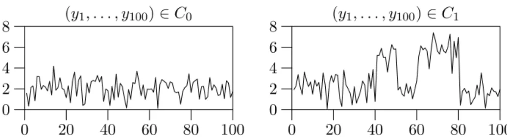
Fraud data used in this thesis is filtered from a database of call data using a velocity trap detection mechanism. An important consequence of this is that the data does not contain information on which calls were fraudulent or which periods contained fraudulent activity. Data labeled as fraudulent is a sample from amixtureof normal and fraudulent data, the mixing coefficients being unknown and changing in time. The setting of data is illustrated in Figure 3.1. Therefore, call data is labeled to classes fraud and normal on a subscriber basis. No geographical information about the calls was available in the call data nor when the velocity trap gave an alarm. The database of fraudulent behavior contained call data of 304 subscribers during a period of 92 days. The normal call data spanned a period of 49 days and was assumed to contain no fraudulent activity. The number of users used in the publications was limited by the available resources. The use of the data may vary in the publications. Consult individual publications for details.
(y1, . . . , y100)∈C0 0 20 40 60 80 100 0 2 4 6 8 (y1, . . . , y100)∈C1 0 20 40 60 80 100 0 2 4 6 8
Figure 3.1: Examples of mixture data. In the left panel, the data belongs to class C0, which has a Gaussian distributionµ1 = 2, σ21 = 1. In the right panel, the data is labeled to belong to the class C1, since it contains data with a Gaussian distribution µ2 = 5, σ22 = 1, representative of class C1. The data from this density is located at t = 40, . . . ,50 and t = 60, . . . ,80. However, these regions are not known in the data. This generated data illustrates the partially labeled call data used in this thesis: normal users are always normal, but fraudulent users behave sometimes normally and sometimes in a fraudulent fashion.
3.2
Representation of call data
Call records constituting the call data are transactions (or events) ordered in time. Each of the call records has a set of call attributes as described earlier. These attributes need to be converted to a form that is compatible with the model used. This conversion can take many forms. Three different data representations are used in this thesis.
3.2.1 Features through aggregation in time
In pattern recognition applications, the usual way to create input data for the model is through feature extraction. In feature extraction, descriptors or statistics of the domain are calculated from raw data. Usually, this process involves some form of aggregation.
In Publication 2 (Taniguchi, Haft, Hollm´en, and Tresp 1998), the de-tection is based on feature variables derived from call data. The unit of aggregation in time is one day. The feature mapping transforms the trans-action data ordered in time to static variables residing in feature space. The features used reflect the daily usage of an account. Number of calls and summed length of calls to describe the daily usage of a mobile phone were used. National and international calls were regarded as different categories. Calls made during business hours, evening hours and night hours were also separated to sub-categories.
3.2.2 Dynamic description of call data
There is a connection between the length of the aggregation period used in feature extraction and the richness of description. It is interesting to consider representations that describe the instantaneous behavior of mobile phone subscribers by pushing the length of the aggregation period to the minimum at the price of a representational richness. In Publication 3 (Hollm´en and Tresp 1999), this kind of representation is used. The call data is sampled for one minute intervals, and the data indicates whether a mobile phone is used during a particular minute. The data for the minutetis then represented withyt∈ {0,1}.
This representation describes the instantaneous calling behavior of mo-bile phone subscribers and permits the dynamic modeling of the calling behavior expressed with transitions from one time step to another. This representation is also the basis of modeling in Publication 4 (Hollm´en, Tresp, and Simula 1999) and Publication 7 (Hollm´en, Tresp, and Simula 2000).
3.2.3 Switching representation
In essence, the feature variables mediate information from the domain to the model used. Sometimes, the model class is limited to certain representations, like categorical data or metric data. In order to avoid compromising how the domain is described, models may be extended to handle data with a more unconventional representation.
The issue of changing representations between metric data and event-based data is reported in Publication 6 (Hollm´en and Tresp 2000). The fact that the data is switching between the continuous and the categorical representations is an artifact of a feature extraction process. When a faithful mapping of the domain is sought for, like in the user profiling problem, extending the model class becomes necessary. The extension is presented in the case of a hidden Markov model (Baum 1972; Juang and Rabiner 1991; Bengio 1999).
User profiling and
classification
This chapter introduces the user profiling and classification methods used for fraud detection. The purpose is to place the novelties found in the publi-cations in a broader framework. The work on finite mixture models, hidden Markov models and hierarchical regime-switching models can be nicely de-scribed in the frameworkof probabilistic networks and therefore the concepts are presented on a general level. Learning in the maximum likelihood frame-workwith the EM algorithm is also presented. In the sequel, Self-Organizing Maps and Learning Vector Quantization are presented with the appropriate extensions. The chapter proceeds with cost-sensitive classification meth-ods and technical assessment methmeth-ods for the fraud detection domain. The chapter ends with a discussion on the presented methods for fraud detection articulating their advantages and disadvantages.
4.1
Probabilistic networks
Probabilistic networks allow an efficient description of multivariate proba-bility densities (Cowell, Dawid, Lauritzen, and Spiegelhalter 1999). Proba-bilistic formulations allow quantifying uncertainty in the conclusions made about the problem, which makes the framework of probabilistic networks ap-pealing for real-world problems. Of particular interest here are the Bayesian networks (Cowell et al. 1999; Jensen 1996), which can be represented as directed acyclic graphs (DAG). A Bayesian networkmay be represented as a graph G = (V, E), where V is the set of vertices or nodes and E is the set of arcs, which is defined as an ordered set of vertices E ⊂V ×V. The nodes of the graph correspond to the domain variables and an arc to the qualitative dependency between two variables (see Figure 4.1).
Graphical representation makes it easy to understand and manipulate networks. The term graphical model refers to this dual representation of
x1 x2
x3 x4 x5
Figure 4.1: A simple Bayesian networkis shown. Variables are marked with graph nodes, the dependency relationships as arcs. The joint probability density can be factorized as P(x1, x2, x3, x4, x5) =
P(x1)P(x2)P(x3|x1)P(x4|x2, x1)P(x5|x2).
probabilistic models as graphs. In the following sections, the concept of conditional independence is briefly described. It is used in defining qualita-tive relationships between the variables, whereas the distributional assump-tions define the quantitative aspect of the probabilistic networks. Learning from data is then briefly described within the frameworkof maximum likeli-hood using the EM algorithm (Dempster, Laird, and Rubin 1977; McLahlan 1996).
4.1.1 Conditional independence
A problem domain consists of a set of random variables. A random variable is an unknown quantity that can take on one of a set of mutually exclusive and exhaustive outcomes (Cowell et al. 1999). The joint probability den-sity P(x1, . . . , xn) of the random variables x1, . . . , xn can be decomposed according to the chain rule of probability (Equation 4.1) as
P(x1, . . . , xn) = n i=1
P(xi|xi−1, . . . , x1). (4.1) Each term in this factorization is a probability of a variable given all lower numbered variables. In real life, however, not all factors influence the others in a given domain, thus this kind of qualitative knowledge can be formu-lated by assuming conditional independence relations between the domain variables. The use of conditional independence assumptions allows one to construct global joint distribution from a set of local conditional probability distributions. Definingπi ⊆ {x1, . . . , xi−1} as the parent set ofxi or the set of variables that renders xi and {x1, . . . , xi−1} conditionally independent, the joint probability density can be written as
P(x1, . . . , xn) = n i=1
P(xi|πi). (4.2) A Bayesian networkdefines this joint probability density as the product of local, conditional densities. The main contribution of the conditional
independence assumptions is that the expression for the joint probability density in Equation 4.2 is simpler than the trivial decomposition achieved by the application of chain rule of probability in Equation 4.1.
4.1.2 Distributional assumptions
Conditional independence assertions provide qualitative assumptions be-tween variables in the probabilistic network. To further quantify these es-tablished relationships, one needs to define for every variable in the network the conditional probability distribution of the variable given its parents. Us-ing classic estimation theory (Cherkassky and Mulier 1998), the probability distributions are specified to come from a parameterized family of distribu-tions. In estimation, the parameters are determined so that the distribution approximates the distribution of the data.
If the observations in each component of a finite mixture model are distributed according to a Gaussian (normal) distribution, it is called the Gaussian mixture model (Redner and Walker 1984; Bishop 1996). In this thesis, this kind of model was used in Publication 2 (Taniguchi, Haft, Hollm´en, and Tresp 1998) to model the probability density of recent calling behavior to be used in novelty detection to detect changes in behavioral pat-terns. Discrete states in the models are best modeled with the assumption of multinomial distributions, in which the variable can be in one of many states of the variable. Exponential distribution was used for modeling call lengths inPublication 6(Hollm´en and Tresp 2000).
Sometimes, the distribution of data may be thought to change from one representation to another. This situation was examined inPublication 6 (Hollm´en and Tresp 2000), where the representation of the data switched from a continuous to a discrete case due to an artifact in the pre-processing of data. The data is augmented with its semantics and a solution to de-couple the data and its semantics is presented. The semantics of the data, which is known, enables choosing the right model for the present data. The method incorporates deterministic switching between data distributions and essentially decouples the different semantics and data from each other. The temporal process of generating different data semantics becomes an integral part of the user profiles.
4.1.3 Learning by EM algorithm
Learning is the process of estimating the parameters of a model from the available set of data. In the context of probabilistic models, it is natural to consider the principle of maximum likelihood. The maximum likelihood estimate for the parameters maximizes the probability of the data for a given model. This is relatively straightforward if the variables in the model are observed, but becomes somewhat complicated, since the models of interest
here include hidden variables. This problem may be overcome by application of the EM algorithm. The EM algorithm (Dempster, Laird, and Rubin 1977; McLahlan 1996) is an iterative algorithm for estimating maximum likelihood parameters in incomplete data problems. Incomplete data means that there is a many-to-one mapping between the hidden state space and the observed measurements. Since it is impossible to recover the hidden variable, EM algorithm works with its expectation instead by making use of the measurements and the implied form of the mapping in the model. The EM algorithm is guaranteed to converge monotonically to a local maximum of the likelihood function (Dempster, Laird, and Rubin 1977; Wu 1983; Xu and Jordan 1996).
For the purpose of the EM algorithm, the expected log likelihood of the complete data (Dempster, Laird, and Rubin 1977) is introduced as
Q(φ|φ(old)) =E(logP(Y, S|φ)|Y, φ(old)) =
S
logP(Y, S|φ)P(S|Y, φ(old))dS, (4.3)
where the log-likelihood of the complete data is parameterized by the free parameter value φ and the expectation is taken with respect to the second distribution parameterized by the current parametersφ(old). In the E-step, theQ function in Equation 4.3 is computed. In Bayesian networks, this is achieved through inserting observed evidence in the networkand applying propagation rules (Jensen 1996) to form the joint probability distribution of all variables or any marginalization of it. The first account that used inference techniques in the E-step appeared in (Lauritzen 1995). In the M-step, the parameter values are updated to be
φ(new)= arg max φ Q(φ|φ
(old)). (4.4) A solution to this maximization problem is usually found by setting the derivatives of the maximized function to zero and solving forφ. The appli-cation of the EM algorithm in the case of mixture models can be found in the literature (Redner and Walker 1984; Bishop 1996). Interestingly, the learn-ing technique used in HMM (Baum 1972) turns out to be an instance of the EM algorithm. Learning in regime-switching models within the framework of maximum likelihood was formulated by Hamilton (1990, 1994). He used a regime-switching model to identify recession periods in the US economy. In Publication 3 (Hollm´en and Tresp 1999), exact inference rules for the hierarchical regime-switching model are derived from the junction tree algo-rithm of the Bayesian networks (Jensen 1996). A recent account on learning from data with graphical models can be found in (Heckerman 1999).
4.1.4 Finite mixture models
In finite mixture models (Everitt and Hand 1981; Redner and Walker 1984; Titterington et al. 1985), one assumes an observed variableY that is condi-tioned on a discrete hidden variableS. The observed variable may be either discrete or continuous. The joint probability density is then
P(S, Y) =P(S)P(Y|S). (4.5) Integration (summation) over the hidden variable S gives an equation for calculating the likelihood of observed data in a more recognizable form as
P(Y) = kj=1P(S = j)ni=1p(yi|S = j). Graphical illustration is shown in Figure 4.2.
. . . S
y1 y2 yn
Figure 4.2: A mixture model is shown. The observed variable Y = (y1, . . . , yn)T is conditioned on a discrete hidden variableS. Observed sam-ples are assumed to be independent.
A Gaussian mixture model was used in Publication 2 in modeling of users’ recent behavior using feature data describing daily usage. After esti-mating a general model from a database of user data, the model is allowed to specialize to individual user profiles by estimating the mixing proportions of the component densities P(S =j) on-line as more call data becomes avail-able. Other parameters are considered to be fixed. The on-line estimation is due to Nowlan (1991). The main result of thePublication 2is that with this approach one is able to detect fraud accurately based on daily usage data.
4.1.5 Hidden Markov models (HMM)
A more complicated model that takes time dependencies into account is the hidden Markov model (HMM), which is widely used in sequence processing and speech recognition (Baum 1972; Juang and Rabiner 1991; Bengio 1999). Smyth et al. (1997) consider HMMs in a general frameworkof probabilistic independence networks and show that algorithms for inference and learning are special cases of more general class of algorithms. For a review on HMM, see (Levinson et al. 1983; Poritz 1988). These models assume a discrete, hidden state st, observations yt that are conditioned on the hidden state as P(yt|st) and the state transitions as P(st|st−1). The joint probability
density is then P(Y, S) =P(y0, s0) T t=1 P(st|st−1;θ1) T t=1 P(yt|st;θ2), (4.6) where the current state is conditionally independent of the whole history given the previous stateP(st|st−1, st−2, . . . , s1) =P(st|st−1). This is called the Markov property, which is prevalent in many kinds of time-series models. Moreover, the current observation is conditionally independent of the whole history given the current hidden state. In essence, the state information summarizes the whole history. The graphical presentation of the HMM is shown in Figure 4.3.
s1 s2 s3 s4 s5
y1 y2 y3 y4 y5
Figure 4.3: In a hidden Markov model, one assumes a hidden variable st
that obeys transitions in time defined by P(st|st−1). The observations are conditioned on the hidden variable as P(yt|st).
In Publication 6 (Hollm´en and Tresp 2000), an HMM was extended to handle a switching representation between metric and event-based data. The model introduces a variable, which determines the correct interpretation of data (see Figure 4.4). The idea is to decouple the occurrence of different
s1 s2 s3 s4 s5
y1 y2 y3 y4 y5
y1∗ y2∗ y∗3 y∗4 y∗5
Figure 4.4: Extended version of the HMM that enables modeling of data streams switching between metric and event-based data. The introduced variable yt∗ determines the correct density to be used in interpreting the likelihood of observed data.
data semantics and the data itself. The observed data semantics expresses whether the data is to be interpreted as metric or event-based. The data semantics forms a dimension of its own in the user profile. The ideas are
illustrated in the case of hidden Markov model, for which inference and learning rules are developed.
4.1.6 Hierarchical regime-switching model
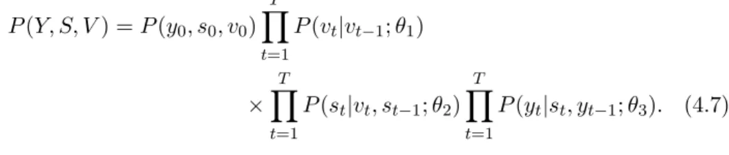
InPublication 3(Hollm´en and Tresp 1999), a more complicated structure is used, which differs from HMM in two aspects. First, the hidden variable that develops in time has a hierarchical structure and second, the proba-bility density for the observations is dependent on past observations. The hierarchical organization involves two layers of states, each of which develops in time according to a Markov chain and the middle layer is conditioned on the layer above. In all, the joint probability for observations and the hidden states (V in the top layer and S in the middle layer, see Figure 4.5) is
P(Y, S, V) =P(y0, s0, v0) T t=1 P(vt|vt−1;θ1) ×T t=1 P(st|vt, st−1;θ2) T t=1 P(yt|st, yt−1;θ3). (4.7) The idea in regime-switching models is to model a problem domain with multiple models allowing the generating mechanism to switch from one mode of operation to another in an indeterministic fashion (Quandt 1958; Quandt and Ramsey 1972; Shumway and Stoffer 1991; Hamilton 1990; Hamilton 1994).
v1 v2 v3 v4 v5
s1 s2 s3 s4 s5
y1 y2 y3 y4 y5
Figure 4.5: Hierarchical regime-switching model is shown. Hidden variables
v and s have a hierarchical structure and middle layer is conditioned on the top layer. Furthermore, observations yt are conditioned on a previous observation yt−1 and the current fraud statest.
InPublication 3, the motivation for introducing hierarchy in the model is to model fraud at different time scales. The middle layer would model fraud as expressed in the call data and the top layer would model whether the account is victimized, that is, whether the fraudster could call if he chose to. The maximum likelihood framework is used in training; additionally gradient
based training is used to enhance the discriminative nature of the model. The results demonstrate the feasibility of the methods in fraud detection. Despite the difficult set up of the problem, the model is able to detect over 90 % of the fraudsters with a false alarm probability of 2 %.
4.2
Self-Organizing Map (SOM)
4.2.1 SOM algorithm
The Self-Organizing Map (SOM) is a neural networkmodel for the analysis and visualization of high-dimensional data. It was invented by Academician Teuvo Kohonen (1981, 1990, 1995) and is the most popular networkmodel based on unsupervised, competitive learning. Self-Organizing Map has been used in a wide range of applications (Kaski et al. 1998). It has also been applied for the analysis of industrial processes (Kohonen, Oja, Simula, Visa, and Kangas 1996; Alhoniemi, Hollm´en, Simula, and Vesanto 1999; Simula, Vesanto, Alhoniemi, and Hollm´en 1999). Earlier workon process monitoring can be seen as the groundworkleading to the problem of fraud detection, which may be seen as auser monitoring problem. InPublication 1, work on the process modeling and monitoring problem is reported.
The Self-Organizing Map is a collection of prototype vectors, between which a neighborhood relation is defined. This neighborhood relation defines a structured lattice, usually a two-dimensional, rectangular or hexagonal lat-tice of map units. After initializing the prototype vectors with, for example, random values, training takes place. Training a Self-Organizing Map from data is divided into two steps, which are applied alternately. First, a best-matching unit (BMU) or a winner unitmc is searched, which minimizes the Euclidean distance between a data samplexand the map units mk
c= arg min
k x−m
k. (4.8)
Then, the map units are updated in the topological neighborhood of the winner unit. The topological neighborhood is defined in terms of the lattice structure, not according to the distances between data samples and map units. The update step can be performed by applying
mk(t+ 1) :=mk(t) +α(t)hc(t, k)[x(t)−mk(t)], (4.9) where the last term in the square brackets is proportional to the gradient of the squared Euclidean distanced(x, mk) =x−mk2. The learning rate
α(t) ∈ [0,1] must be a decreasing function of time and the neighborhood function hc(t, k) is non-increasing function around the winner unit defined in the topological lattice of map units. A good candidate is a Gaussian around the winner unit defined in terms of the coordinates r in the lattice
of neurons hc(t, k) = exp −rk−rc2 2σ(t)2 . (4.10)
During learning, the learning rate and the width of the neighborhood func-tion are decreased, typically in a linear fashion. In practice, the map then tends to converge to a stationary distribution, which reflects the properties of the probability density of data.
The Self-Organizing Map may be visualized by using a unified distance matrix representation (Ultsch and Siemon 1990), where the clustering of the SOM is visualized by calculating distances between the map units locally and representing these visually with gray levels. Another choice for visualization is the nonlinear Sammon’s mapping (Sammon Jr. 1969), which projects the high-dimensional map units on a plane by minimizing the global distortion of inter point distances.
4.2.2 SOM in process monitoring
Self-Organizing Map has found many applications in industrial environments (Kohonen, Oja, Simula, Visa, and Kangas 1996). Early workon monitor-ing the state of an industrial process is reported in (Tryba and Goser 1991; Kasslin, Kangas, and Simula 1992). The goal in process monitoring is to develop a representation of the state of an industrial process from process data and to use this representation in monitoring the current state of the process. Although conceptually operating on a different level, the problem of process monitoring is similar to the problem of monitoring users. In pro-cess monitoring, the focus is on the system level, whereas in user monitoring problems, the users are thought to form individual processes to be moni-tored. The problem of activity monitoring focusing on the level of users is also articulated by Fawcett and Provost (1999). The workin the area of pro-cess monitoring is reported inPublication 1(Alhoniemi, Hollm´en, Simula, and Vesanto 1999) and also in (Simula, Alhoniemi, Hollm´en, and Vesanto 1997; Simula, Vesanto, Alhoniemi, and Hollm´en 1999; Simula, Ahola, Al-honiemi, Himberg, and Vesanto 1999). This worklays the groundworkfor the later workin user profiling and classification problems.
In the simple example presented inPublication 1(Alhoniemi, Hollm´en, Simula, and Vesanto 1999), a computer system is monitored in terms of its internal state measured by its central processor unit (CPU) activity as well as its networkconnections. The analysis begins by collecting the time-dependent measurements in a measurement vector and by pre-processing them appropriately. By training a Self-Organizing Map from the measure-ments, different states of the system may be visualized and the current state may be mapped to the characterized states for understanding the behavior of the process. Although the authors were ignorant of the workin intrusion
detection at the time the workwas done, the workbears some analogs, at least conceptually.
4.2.3 SOM for clustering probabilistic models
Publication 4presents a Self-Organizing Map algorithm, which enables us-ing probabilistic models as the cluster models. In this approach the map unit indexed by kstores the empirically estimated parameter vector θk with an associated probabilistic modelq(x;θk). For implementing a Self-Organizing Map algorithm, one needs to define a distance between the map units (i.e. the θk) and data. The distance betweenθ and a data point itself can not be defined in Euclidean space since they may have different dimensional-ity. The most common distance measure between probability distributions is the Kullback-Leibler distance (Bishop 1996; Ripley 1996), which relates two probability distributions. If one considers the data samplexi to be dis-tributed according to an unknown probability distributionxi ∼ p(x) then one may approximate p(x) ≈ δ(x−xi) by placing a unit impulse δ(x) at the data point. If this expression is substituted into the Kullback-Leibler distance, one gets
KL(pq) =− p(x) logq(x;θ k) p(x) dx⇒ −logq(xi;θ k), (4.11)
which is the negative log probability of data for the empirical model. Thus, minimizing the Kullback-Leibler distance between the unknown true distri-bution that generated the data point at hand and the empirical model leads to minimizing the negative logarithm of the probability of the data with the empirical model. This justifies the use of this probability measure as a distance measure between models and data. In light of this derivation, one can derive a Self-Organizing Map algorithm for parametric probabilistic models. A winner unit indexed by c is defined by minimizing the negative log-likelihood of the empirical models for a given data point or equivalently, by searching for the maximum likelihood unit as in
c= arg min
k [−logq(xi;θ
k)] = arg max
k q(xi;θ
k). (4.12)
The update rules are based on the gradients of this likelihood in the topo-logical neighborhood of the winner unitc as
θk(t+ 1) :=θk(t) +α(t)hc(t, k)∂logq(x(t);θ k)
∂θk . (4.13) To illustrate the idea, an algorithm for a specific case of user profiling in mobile phone networks is derived inPublication 4.
4.3
Learning Vector Quantization (LVQ)
4.3.1 LVQ algorithm
The Learning Vector Quantization algorithm (Kohonen 1990; Kohonen 1995; Kohonen, Hynninen, Kangas, Laaksonen, and Torkkola 1996) estimates a classifier from labeled data samples. The classifier consists of a labeled set of codebookvectors, and the classification is based on the nearest-neighbor rule. Thus, the method does not, in contrast to traditional vector quantiza-tion or SOM, approximate the class densities, but defines the class borders by the placement of class-specific codebookvectors (Kohonen 1995). This approach is also motivated by the observation that in a discrimination task a good estimate for the class density is only needed near the class border. In the training phase, for a random samplex, there is a winner unit among the codebookvectorsmk defined by
c= arg min
k x−m
k. (4.14)
This winner unitmc is adapted in order to decrease the expected misclassi-fication probability for the training set according to
mc(t+ 1) :=mc(t)±α(t)[x(t)−mc(t)]. (4.15) The sign is chosen according to the correctness of the classification. If the label of the training sample matches that of the nearest codebookvector, the sign + is chosen, otherwise−is chosen. In LVQ, only the winner unit is updated, in contrast to the SOM algorithm, where a neighborhood function around the winner determines the map units to be updated. The class border defined by the codebookvectors and the nearest-neighbor classification rule approximates the Bayes’ decision surface (Kohonen 1995).
4.3.2 LVQ for probabilistic models
In LVQ, the class border is defined by codebookvectors, which are proto-types in the input space. If representing data by protoproto-types is infeasible, one may replace the concept of a prototype by data generating models. This has been considered inPublication 7(Hollm´en, Tresp, and Simula 2000), which extends the ideas in Publication 4 (Hollm´en, Tresp, and Simula 1999) to the classification domain. As far as the distance measures are concerned, the same reasoning applies to the LVQ algorithm as does for the SOM algorithm (Equation 4.11). Relating empirical models and the unknown densities be-hind the data samples with the Kullback-Leibler distance measure leads to the negative logarithm of the probability of data samples with the empir-ical models. Therefore, as in the case of the SOM algorithm, the winner search looks for a maximum likelihood unit indexed bycas in the Equation 4.12. The update is based on the gradient update of the winner unit. The