Airline Planning and Schedule
Development
Timothy L. Jacobs, Laurie A. Garrow, Manoj Lohatepanont, Frank S. Koppelman, Gregory M. Coldren, and Hadi Purnomo
2.1 Introduction and Scope
Airlines have evolved over the past 70 years from simple contract mail carriers into sophisticated businesses. The current airline environment is very competitive and dynamic. Maintaining consistent profitability requires that appropriate trade-offs be made between the often competing objectives within planning, marketing and operations. Airlines have led other industries in the application of operations research and information technology to deal with these issues. The real-time solution of large-scale optimization models has played a significant role in shaping today’s airline industry. This role will increase as the industry becomes more competitive and flight characteristics change due to the implementation of new technologies. Airline planning and scheduling represents an excellent example of the application of operations research and mathematical modeling to solve com-plex and real industry problems.
2.2 Overview of Airline Schedule Planning and Marketing
Planning and Marketing define an airline’s products and determine how they will be sold. This is a continuous process which begins 5 or more years before a flight’s departure and operates until the last passenger is boarded and the aircraft door is
T. L. Jacobs (&)L. A. GarrowM. LohatepanontF. S. Koppelman
G. M. ColdrenH. Purnomo e-mail: [email protected] L. A. Garrow
e-mail: [email protected]
C. Barnhart and B. C. Smith, LLC (eds.),Quantitative Problem Solving Methods in the Airline Industry, International Series in Operations Research & Management Science 169, DOI: 10.1007/978-1-4614-1608-1_2,Springer Science+Business Media, LLC 2012
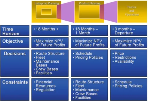
closed. This process can be viewed as a series of overlapping sequential steps that include scheduling, marketing and distribution. This process requires an exchange of data and feedback between scheduling, pricing and revenue management and distribution. In addition, other considerations such as crew resources, maintenance and engineering and ground services help define the boundaries by which the airline schedule must operate and be managed (Fig.2.1).
Schedulingdetermines where and when the airline will fly. Schedules are built to maximize long-term profitability. The revenue and cost associated with each schedule are based on very different views of the same information. Although the schedule is composed of individual flight legs between two cities, the airline’s product and revenues are based on passenger origin and destination (O&D) mar-kets. An O&D market is defined by a passenger’s point of entry and exit from the airline system. The schedule is built to maximize its attractiveness to customers in a wide variety of O&D markets. The development of hub and spoke networks was based on providing maximum O&D coverage with a limited number of flight legs. The costs of operating the schedule depend on the flight legs, which drive the number and type of aircraft used. The schedule must consider the cost and availability of cabin and flight deck crews, as well as the requirement that aircraft cycle through maintenance bases at regular intervals. As a result, the schedule also determines the location and size of ground facilities, and the number and location of crew and maintenance bases.
Fig. 2.1 Schedule planning and operation timeframe, objectives and constraints (Smith and Jacobs1997)
Efficient schedules which match supply and demand are key to airline profit-ability. Profitable solutions require anticipation of general market conditions: the costs of capital, fuel and labor, as well as the level and nature of competition. Airlines address many scheduling issues (assigning aircraft and crews to flights, routing aircraft to maintenance bases) with large-scale combinatorial optimization techniques. The scale of today’s airlines makes this increasingly difficult. For example, large U.S. domestic carriers operate more than 3,000 flights per day with 600 or more aircraft and can include more than 300 cities, serving over 10,000 unique O&D markets.
Marketingdetermines what specific products will be offered for sale and how many of each will be sold. The two primary components of airline marketing are pricing and yield management. Since deregulation of the U.S. domestic airline industry, both have evolved into very complex processes. Prior to deregulation, individual airlines served specific market segments. Scheduled carriers served the business traveler while charter carriers served the leisure market. Scheduled carriers flew with relatively low load factors but remained reasonably profitable due to the limited competition created by government regulation.
Just prior to deregulation, the scheduled carriers started to offer additional products to the leisure market segment to help fill some of the empty seats. There were two problems with this approach. First, airline revenue would have been severely diluted if the existing customer base switched from full fare to discounts. Restrictions were introduced to make discounts unappealing to existing business travelers (advance purchase, saturday night stay). Second, some flights were already full and discount sales would displace late booking, high value traffic. The yield management process was introduced shortly after deregulation to anticipate where discount sales would and would not be profitable. From this simple beginning, the pricing and yield management process has become very complex and dynamic. Their combined role is to help airlines fine tune demand and sales to meet the capacity provided by the schedule. Today, a U.S. domestic carrier’s schedule can consist of up to 4 million fares. These fares and restrictions are adjusted frequently to match demand to supply; 100,000 fare changes per day is typical. As a result, revenue management departments must keep up with these changes. Every day the number of reservations available for sale is reviewed and adjusted in order to maximize total revenues on all future flights. This is another very large-scale optimization process that involves solving a highly stochastic and nonlinear optimization model. Con-trolling reservation availability for all future flights at a large U.S. carrier can rep-resent a problem with approximately 500 million decision variables.
Distributionis the process of taking the airline products and putting them on the shelf for sale. The store front for the airline industry is primarily central reservation systems (CRS) and global distribution systems (GDS). A CRS allows an airline’s reservation agents to book their own flights and fares. CRSs are relatively expensive to develop and maintain. Large airlines typically have their own CRS, while second and third tier carriers tend to rent space in another carrier’s (often their competitor’s) system. In the 1970s U.S. domestic carriers began to give travel agents access to their CRSs. This provided each airline with a method for selling products outside of the
reservations office. Through the 1980s the number of travel agents with direct access to the major CRSs (Sabre, Apollo-United Airlines, Galileo-British Airways, World Span) grew substantially. Each CRS became a significant distribution outlet not only for the originating airline but for other participating airlines. Today the successors to these CRSs have become global in that an agent hooked into Sabre or Amadeus has access to the schedules, fares and reservation availability for most of the world’s airlines. This gives any airline immediate access to a very significant distribution process. For example, Sabre contains schedules for over 700 airlines and agents can book tickets directly on 350 airlines. Sabre is installed in over 29,000 travel agency locations and processes more than 4,900 messages per second.
2.3 Chapter Outline
This chapter will focus on the application of forecasting and operations research techniques to airline scheduling problems and provide a brief overview of how airlines use these techniques to develop and evaluate schedules and business decisions.Section 2.2of this chapter provides a brief overview of the forecasting process used to estimate passenger demand and determine the expected revenue, cost and profitability associated with a given schedule. This section will also provide insight as to how airlines use these techniques to evaluate incremental changes to market services such as frequency and/or aircraft assignment changes.
Section 2.3provides an overview of the fleeting process used by most network carriers. This section presents an introduction to the fleet assignment model (FAM) and some of the enhancements to the model better integrate the schedule devel-opment and fleeting processes with both operational and revenue management aspects of the airline business process. These enhancements will include the incorporation of O&D passenger effects (O&D FAM) and the inclusion of high-level maintenance and engineering (M&E) opportunities into the schedule development and fleeting process.Section 2.4will provide a high-level overview of the aircraft routing process and its impact on other business units within the company such as M&E and flight and ground crew resources.Section 2.5presents an overview of some new developments and directions in the operations research and forecasting and their application to the airline scheduling area. Section 2.6
provides a full list of references noted within the chapter for further study.
2.4 Forecasting Aspects and Methodologies
for Schedule Planning
This section includes three major components. First, an overview of the data and major components of network-planning models is presented. Next, the two major types of market share models based on the Quality of Service Index (QSI)
methodology or logit-based methodologies are reviewed. This is followed by a summary of the key experiences of a major U.S. airline that transitioned from using an itinerary choice model based on a QSI methodology to one based on a logit methodology. The section concludes with a discussion of one relatively new modeling technique: the use of continuous time-of-day functions (versus discrete time-of-day dummy variables or schedule delay functions). Part of the material in this section is reprinted from Garrow (2010, pp. 203–208, 228–229, 250) with permission from Ashgate Publishing. The material draws heavily on prior work from Coldren and Koppelman as well as information obtained via interviews with industry experts.
2.4.1 Introduction
Network-planning models (also called network-simulation or schedule profitability forecasting models) are used to forecast the profitability of airline schedules. These models support many important long- and intermediate-term decisions. For example, they aid airlines in performing merger and acquisition scenarios, route schedule analysis, code-share scenarios, minimum connection time studies, price-elasticity studies, hub location and hub buildup studies and equipment purchasing decisions. Conceptually, ‘‘network-planning models’’ refer to a collection of models that are used to determine how many passengers want to fly, which itineraries (defined as a flight or sequence of flights) they choose, and the revenue and cost implications of transporting passengers on their chosen flights.
Although various air carriers, aviation consulting firms and aircraft manufac-turers own proprietary network-planning models, very few published studies exist describing them. Further, because the majority of academic researchers did not have access to the detailed ticketing and itinerary data used by airlines, the majority of published models are based on stated preference surveys and/or a high level of geographic aggregation. These studies provide limited insights into the range of scheduling decisions that network-planning models must support. Recent work by Coldren and Koppelman provides some of the first details into network-planning models used in practice (Coldren2005; Coldren and Koppelman2005a,
b; Coldren et al.2003; Koppelman et al.2008).
2.4.2 Overview of Major Components of Network-Planning
Models
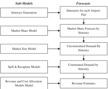
As shown in Fig.2.2, ‘‘network-planning models’’ refer to a collection of sub-models. First, an itinerary generation algorithm is used to build itineraries between each airport pair using leg-based air carrier schedule data obtained from a
source such as the Official Airline Guide (OAG Worldwide Limited2010). OAG data contain information for each flight including the operating airline, marketing airline (if a code-share leg), origin, destination, flight number, departure and arrival times, equipment, days of operation, leg mileage and flight time. Itineraries, defined as a flight or sequence of flights used to travel between the airport pair, are constructed from the OAG schedule. Itineraries are usually limited to those with a level-of-service that is either a non-stop, direct (a connecting itinerary not involving an airplane change), single-connect (a connecting itinerary with an airplane change) or double-connect (an itinerary with two connections). For a given day, an airport pair may be served by hundreds of itineraries, each of which offers passengers a potential way to travel between the airports. Although the logic used to build itineraries differs across airlines, in general itinerary generation algorithms include several common characteristics. These include distance-based circuitry logic to eliminate unreasonable itineraries and minimum and maximum connection times to ensure that unrealistic connections are not allowed. In addi-tion, itineraries are typically generated for each day of the week to account for day-of-week differences in service offered.
An exception to the itinerary generation algorithm described above was developed by Boeing Commercial Airplanes for large-scale applications used to allocate weekly demand on a world-wide airline network. In this application, a weekly airline schedule involves the generation of 4.8 million paths across 280,000 markets that are served by approximately 950 airlines with 800,000 flights. Boeing’s algorithms, outlined in Parker et al. (2005), integrate discrete choice theory into both the itinerary generation and itinerary selection. That is, the
Forecasts
Spill & Recapture Models
Itineraries for each Airport-Pair
Market Share Forecast by Itinerary Unconstrained Demand by Itinerary Constrained Demand by Itinerary Revenue Estimates Market Share Model
Market Size Model
Revenue and Cost Allocation Models Model Sub-Models Itinerary Generation
utility value of paths is explicitly considered as the paths are being generated; those paths with utility values ‘‘substantially lower’’ than the best path in a market are excluded from consideration.
After the set of itineraries connecting an airport pair is generated, a market share modelis used to predict the percentage of travelers who select each itinerary in an airport pair. Different types of market share models are used in practice and can be generally characterized based on whether the underlying methodology uses a QSI or discrete choice (or logit-based) framework. Both types of market share models are discussed in this chapter.
Next, demand on each itinerary is determined by multiplying the percentage of travelers expected to travel on each itinerary by the forecastedmarket size, or the number of passengers traveling between an airport pair. However, because the demand for certain flights may exceed the available capacity,spill and recapture modelsare used to reallocate passengers from full flights to flights that have not exceeded capacity. Finally, revenue and cost allocation models are used to determine the profitability of an entire schedule (or a specific flight).
Market size and market share information can be obtained from ticketing data that provide information on the number of tickets sold across multiple carriers. In the U.S., ticketing data are collected as part of the U.S. Department of Trans-portation (U.S. DOT) Origin and Destination Data Bank 1A or Data Bank 1B
(commonly referred to as DB1A or DB1B). The data are based on a 10% sample of flown tickets collected from passengers as they board aircraft operated by U.S. airlines. The data provide demand information on the number of passengers transported between origin–destination pairs, itinerary information (marketing carrier, operating carrier, class of service, etc.) and price information (quarterly fare charged by each airline for an origin–destination pair that is averaged across all classes of service). Although the raw DB datasets are commonly used in academic publications (after going through some cleaning to remove frequent flyer fares, travel by airline employees and crew, etc.), airlines generally purchase ‘‘Superset’’ data from the company Data Base Products (Data Base Products Inc.
2010). Superset data are a cleaned version of the DB data that are cross-validated against other data sources to provide a more accurate estimate of market sizes. See the websites of the Bureau of Transportation Statistics or Data Base Products for additional information.
The U.S. is the only country that requires airlines to report a 10% sample of used tickets. Thus, although ticketing information about domestic U.S. markets is publicly available, the same is not true for other markets. Two other sources of ticketing information include the Airline Reporting Corporation (ARC) and the Billing Settlement Plan (BSP), the latter of which is affiliated with the Interna-tional Air Transport Association (IATA). ARC is the ticketing clearinghouse for many airlines in the U.S. and essentially keeps track of purchases, refunds and exchanges for participating airlines and travel agencies. Similarly, BSP is the primary ticketing clearinghouse for airlines and travel agencies outside the U.S.
Given an understanding of the major components of network-planning models and the OAG schedule, itinerary and ticketing data sources that are required to support the development of these models, the next sections provide a detailed description of QSI and logit-based market share models.
2.4.3 QSI Models
Market share models are used to estimate the probability a traveler selects a specific itinerary connecting an airport pair. Itineraries are the products that are ultimately purchased by passengers, and hence it is the characteristics of these itineraries that influence demand. In making their itinerary choices, travelers make tradeoffs among the characteristics that define each itinerary (e.g. departure time, equipment type(s), number of stops, route, carrier). Modeling these itinerary-level tradeoffs is essential to truly understand air-travel demand and is, therefore, one of the most important components of network-planning models.
The earliest market share models employed a demand allocation methodology referred to as QSI.1QSI models, developed by the U.S. government in 1957 in the era of airline regulation (Civil Aeronautics Board 1970) relate an itinerary’s passenger share to its ‘‘quality’’ (and the quality of all other itineraries in its airport pair), where quality is defined as a function of various itinerary service attributes and their corresponding preference weights. For a given QSI model, these pref-erence weights are obtained using statistical techniques and/or analyst intuition. Once the preference weights are obtained, the final QSI for a given itinerary is usually expressed as a linear or multiplicative function of its service characteristics and preference weights. For example, suppose a given QSI model measures itin-erary quality along four service characteristics (e.g. number of stops, fare, carrier, equipment type) represented by independent variables X1; X2; X3; X4 and their
corresponding preference weights b1; b2; b3; b4: The QSI for itinerary i; QSIi;
can be expressed as:
QSIi¼ðb1X1þb2X2þb3X3þb4X4Þ; or
QSIi¼ðb1X1Þðb2X2Þðb3X3Þðb4X4Þ:
Other functional forms for the calculation of QSI’s are also possible. For itineraryi, its passenger share is then determined by:
Si¼PQSIi
j2J
QSIj
1 QSI models described in this section are based on information in the Transportation Research
Board’s Transportation Research E-Circular E-C040 (Transportation Research Board2002) and on the personal experiences of Gregory Coldren and Tim Jacobs.
where
Si is the passenger share assigned to itineraryi, QSIiis the quality of service index for itineraryi, P
j2J
QSIj is the summation over all itineraries in the airport pair.
Theoretically, QSI models are problematic for two reasons. First, a distin-guishing characteristic of these models is that their preference weights (or sometimes subsets of these weights) are usually obtained independently from the other preference weights in the model. Thus, QSI models do not capture inter-actions existing among itinerary service characteristics (e.g. elapsed itinerary trip time and equipment, elapsed itinerary trip time and number of stops). Second, QSI models are not able to measure the underlying competitive dynamic that may exist among air travel itineraries. This second inadequacy in QSI models can be seen by examining the cross-elasticity equation for the change in the passenger share of itineraryjdue to changes in the QSI of itineraryi:
gSj QSIi ¼ oSj oQSIi QSIi Sj ¼ SiQSIi:
The expression on the right side of the equation is not a function ofj. That is, changing the QSI (quality) of itineraryiwill affect the passenger share of all other itineraries in its airport pair in the same proportion. This is not realistic since, for example, if a given itinerary (linking a given airport pair) that departs in the morning improves in quality, it is likely to attract more passengers away from the other morning itineraries than the afternoon or evening itineraries.
Thus, to summarize, because QSI models have a limited ability to capture the interactions between itinerary service characteristics or the underlying competitive dynamic among itineraries, other methodologies, such as those based on discrete choice models have emerged in the industry. A detailed overview of discrete choice models is provided in the Customer Modeling chapter. An overview of how discrete choice models have been applied to market share modeling is presented in the next section.
2.4.4 Application of Discrete Choice Models to Market Share
Modeling
As presented in the Customer Modeling chapter, discrete choice (or ‘‘logit’’) models such as the multinomial logit (MNL) model are random utility maximizing models that describe how individuals choose one alternative among a finite set of mutually exclusive and collectively exhaustive alternatives. The individual chooses the alternative that has the maximum utility. The utility function for a random utility model is defined as
Uni¼bxni
where
Uniis the total utility of alternative ifor individualn.
bis the vector of parameters associated with attributesx. Utility is assumed to be a linear in parameters function of attributesx.
xniis the vector of attributes that vary across individuals and alternatives. Because the utility the individual receives from each alternative is not known to the researcher, the utility function is assumed to have two components. The sys-tematic or representative component contains observed variables that describe characteristics of the individuals and alternatives. The unobserved or error com-ponent is a random term that represents the unknown (to the researcher) portion of the individuals’ utility function. The utility function is estimated using
Vni¼bxniþeni
where
Vni is the total observed utility of alternativeifor individual n bis the vector of estimates forb
xniis the vector of attributes for alternative iand individualn eniis an unobserved error component.
Different choice models are derived by imposing assumptions about the dis-tribution of the error term and/orb: For example, the assumption that the error term is independent and identically distributed Gumbel2with mode30 and scalec;
iid G(0,c;) leads to the multinomial logit (MNL) model (McFadden 1974). The MNL probability of selecting alternativeiamong alljalternatives inCn, the choice
set for individualn, can be expressed in closed-form as
Pni¼P iðjxni;bÞ ¼ e b0x ni P j eb0xnj :
The main limitation of the MNL is exhibited in the independence of irrelevant alternatives (IIA) property which states that the ratio of choice probabilitiesPni/Pnj
for i, j [ Cn is independent of the attributes of any other alternative. The IIA
property of the MNL model is also apparent by examining the cross-elasticity equation for the change in the probability of itinerary j due to changes in an attribute of itineraryi:
2 An iid Gumbel distribution is also called Type I extreme value.
3 Several publications incorrectly report the parameters describing the Gumbel distribution as
the mean and scale. However, the shape and dispersion of the Gumbel distribution are formally defined by the mode and scale. Further, the mean of the Gumbel is given by the relationship mean=mode?{0.577/c}.
gPj Xik ¼ oPj oXik Xik Pj ¼ PibkXik
Note that the expression on the right side is not a function ofj. The IIA property of MNL is equivalent to the elasticity problem of the QSI model; that is, the cross-elasticity is undifferentiated across alternatives. In terms of substitution patterns, this means a change or improvement in the utility of one alternative will draw share proportionately from all other alternatives. In many applications, this may not be a realistic assumption. For example, in itinerary choice, the unobserved factors associated with the non-stop alternatives are expected to be correlated (since all non-stops are more convenient for passengers, may exhibit a decreased likelihood of lost luggage, etc.). Thus, the substitution between these alternatives is likely to be greater than between any of them and the connecting alternatives.
While the MNL model can be criticized for the restrictive substitution patterns it imposes, recent comparisons of itinerary choice models based on the MNL and QSI methodologies at a major U.S. airline clearly showed that the MNL outper-formed their QSI model. In addition, many other discrete choice models (some developed specifically within the context of airline itinerary choice) can be used to incorporate flexible substitution patterns. Thus, the IIA property should not be viewed as a limitation of discrete choice models, as many other models (discussed extensively in Garrow2010) can be used to relax this property. Nonetheless, it is interesting to note that in the context of itinerary choice models, even the simple MNL model dramatically outperformed the QSI model.
2.4.5 MNL and QSI Model Development at a Major U.S. Carrier
One of the first published studies modeling air-travel itinerary share choice based on a discrete framework was published in Coldren et al. (2003). MNL model parameters were estimated from a single month of itineraries (January 2000) and validated on monthly flight departures in 1999 in addition to selected months in 2001 and 2002. Using market sizes from the quarterly Superset data adjusted by a monthly seasonality factor, validation was undertaken at the flight segment level for the carrier’s segments. That is, the total number of forecasted passengers on each segment was obtained by summing passengers on each itinerary using the flight segment. These forecasts were compared to onboard passenger count data. Errors, defined as the mean absolute percentage deviation, were averaged across segments for regional entities and compared to predictions from the original QSI model. Regional entities are defined by time zone for each pair of continental time zones in the U.S. (e.g. East–East, East-Central, East-Mountain, East–West,… ,-West–West) in addition to one model for the Continental U.S. to Alaska/Hawaii and one model for Alaska/Hawaii to the Continental U.S. The MNL forecasts were consistently superior to the QSI model, with the magnitude of errors reduced on the order of 10–15% of the QSI errors. Further, forecasts were stable across
months, including months that occurred after September 11, 2001. Additional validation details and estimation results are provided in Coldren et al. (2003).
The MNL itinerary share model reported in Coldren et al. (2003)—which represents a discrete choice model that was used to replace a major U.S. airlines’ QSI model—includes variables for level-of-service, carrier presence, connection quality, aircraft size and type, fare and departure time-of-day. The representation of passengers’ preferences for non-stop flights merits further discussion as it is unique from many other specifications found in practice and, more importantly, was found to be robust. Specifically, level-of-service (non-stop, direct, single-connect, or double-connect) is modeled using dummy variables to represent the level-of-service of the itinerary withrespect to the best level of serviceavailable in the airport pair. That is, an itinerary with a double connection is much more onerous to passengers when the best level-of-service in the market is a non-stop than when the best level-of-service in the market is a single connection. Further, parameter estimates across 18 regional entities reveal that passengers have similar, but not identical responses, to changes in level-of-service across the entire domestic system. This is one example of the benefits of a ‘‘well-defined’’ utility function that captures the fundamental trade-offs of how passengers make itinerary choices; that is, parameter estimates are stable across datasets. Subsequently, this aids in transferability across different time periods and leads to better and more stable forecasting accuracy.
Another common industry practice reflected in the MNL itinerary share model of the major U.S. carrier is the inclusion of carrier presence variables. Numerous studies have found that increased carrier presence in a market leads to increased market share for that carrier (Algers and Beser2001; Nako 1992; Proussaloglou and Koppelman 1999; Suzuki et al. 2001). In the MNL model, a ‘‘point of sale weighted airport presence’’ variable, used to represent carrier presence at both the origin and destination, is found to influence the value of itineraries.
Finally, it is important to note that in the major carrier’s MNL itinerary share model, preferences for departure times are represented via the inclusion of time-of-day dummy variables for each hour of the day. In practice, there are other methods based on schedule delay formulations that are currently in use or are being explored in a research context to represent individuals’ time-of-day pref-erences. Unfortunately, the terminology that has been used to describe the sche-dule delay functions is often referred to as a ‘‘nested logit model’’ within the airline community, which is incorrect. The next section clarifies the distinction between time-of-day preference and schedule delay functions. The Customer Choice chapter clarifies the definition of the nested logit model, as derived from discrete choice theory and discusses more advanced discrete choice models that have been applied to itinerary share and other airline applications.
2.4.6 Time-of-Day Preferences Versus Schedule Delay Functions
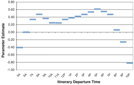
Determining when to schedule flights is arguably one of the most important decisions made by airline scheduling departments. Scheduling flights during unpopular departure times will result in fewer passengers and/or lower average fares. As described in Koppelman et al. (2008), different approaches have been used to model air travelers’ departure time preferences. The first is to include time-of-day dummy variables for each hour of the day. Figure2.3shows an example of time-of-day preferences for a month of continental U.S. departures based on all flights traveling westbound by one time zone. Parameter estimates based on a MNL formulation indicate passengers prefer to depart early in the morning (at 8 a.m.) or later in the afternoon (5 p.m.).
However, the use of discontinuous time periods poses interpretation problems in practice as a slight change in schedule (e.g. from 9:59 p.m. to 10:02 p.m.) can cause large and counter-intuitive shifts in the probabilities. Estimation of param-eters for all time periods can also be subject to over-fitting problems. To address these deficiencies, Koppelman et al. (2008) propose an approach adopted by Zeid et al. (2006) in the context of urban travel activity models. The approach is to estimate weighting parameters for a series of sine and cosine curves to obtain an overall representation of the distribution of departure time preferences. The time-of-day preference for three sine and cosine curves is specified as:
-1.00 -0.80 -0.60 -0.40 -0.20 0.00 0.20 0.40 0.60 0.80 Parameter Estimate
Itinerary Departure Time
Fig. 2.3 Passenger departure time preferences from time period model.SourceReprinted from Koppelman et al. (2008) with permission of Elsevier
Utility for alternativei¼b1sin 2pti 1440 þb2sin 4pti 1440 þb3sin 6pti 1440 þb4cos 2pti 1440 þb5cos 4pti 1440 þb6cos 6pti 1440 where
tiis the departure time of itineraryi expressed as minutes past midnight
1440 is the number of minutes in the day.
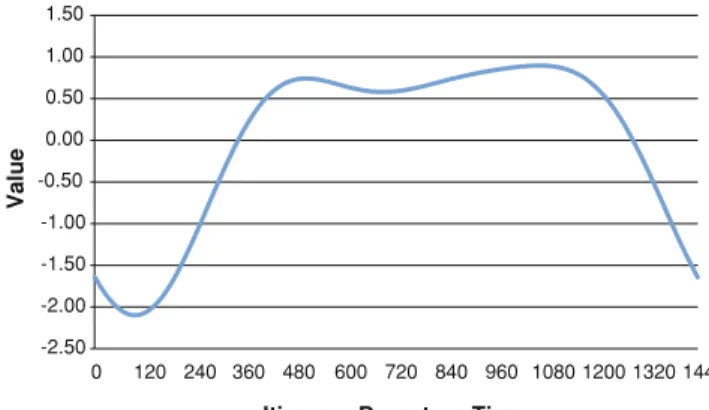
The final time-of-day value from this model is obtained by summing the six weighted trigonometric functions and is shown in Fig.2.4. Statistical tests indicate that continuous specification is preferred over the time-of-day dummy variables.4 Carrier (2008) proposed a modification to this formulation to account for cycle lengths that are shorter than 24 hours. Formally, the equation:
b1sin 2ph 1440 þb2cosin 2ph 1440 þ is replaced with -2.50 -2.00 -1.50 -1.00 -0.50 0.00 0.50 1.00 1.50 0 120 240 360 480 600 720 840 960 1080 1200 1320 1440 Va lu e
Itinerary Departure Time
Fig. 2.4 Time of day utility curve from base sin–cos model.SourceReprinted from Koppelman et al. (2008) with permission of Elsevier
4 Other trigonometric functions involving an additional offset parameter, such as those proposed
by Gramming et al. (2005) were also estimated as part of the analysis. Results from these two approaches were virtually identical.
b1sin 2pðhsÞ d n o þb2cosin 2pðhsÞ d n o þ led24 0se
whereeandlrepresent the departure times of the earliest and latest itineraries in the market, respectively,hrepresents the departure time,srepresents the start time of the cycle (which is not uniquely identified and can be set to an arbitrary value) anddrepresents the cycle duration. The examples in this chapter use the 24-hours period, as Carrier’s formulation leads to a nonlinear-in-parameters function, which he solved using a trial-and-error method. The trial-and-error method (often used by discrete choice modelers when they encounter nonlinear-in-parameters functions) essentially fixesdto different values and estimates the remaining parameters. The value ofdthat results in the best log likelihood value is the preferred model.
Figures2.3and2.4represent time-of-day preferences on a 24-hours cycle by measuring the relative value of a departure time relative to all other possible departure times. However, from a behavioral perspective, itinerary selection may be influenced by an individual’s effort to depart as close as possible to his/her ideal departure time. The difference between an individual’s desired departure time and actual departure time is defined as schedule delay. Formally, schedule delay for itineraryi,SDi, can be expressed as:
SDi¼X
8j
g DTi TPjWTPj
where
DTiis the departure time for itineraryi
TPjis the start of each 15-min time period from 5:30 a.m. to 10:30 p.m.
g() is a transformation function of the difference in minutes between the itinerary departure time and the time period
WTPj is the weight for time periodj.
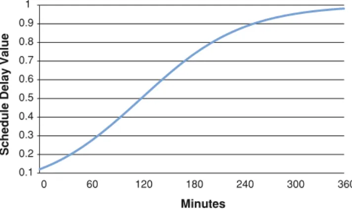
There are two key points to note about this formulation. First, the weightsWTPj account for departure preferences and the distribution of observed passenger departures at different times-of-day. Second, the formulation is general in the sense that different schedule delay transformation functions are possible. Several func-tions, including linear, square root, squared, logistic, etc. were estimated. The logistic transformation shown in Fig.2.5was found to fit the data the best. For-mally, this schedule delay transformation and time period weights are given as:
g DTiTPj ¼ 1 1þexp a2jDTaiTPjj 1 WTPj ¼ sincosValueTPj P j sincosValueTPj
where
DTiis the departure time for itineraryi
TPjis the start of each 15-min time period from 5:30 a.m. to 10:30 p.m.
sincosValueTPj is the sum of the added terms for time periodj.
The formulation based on schedule delay is found to fit the data better than the model based on continuous time-of-day preferences. Additional results that cap-ture differnces in day-of-week deparcap-ture time preferences as well as early and late departure (or arrival) delays by outbound and inbound itineraries are reported in Koppelman et al. (2008).
2.4.7 Summary
This section focused on describing two major types of market share models found in scheduling models: those based on the QSI methodology and those based on discrete choice methods. An emphasis was placed on identifying concepts that in the authors’ experiences are commonly misunderstood in practice. This includes the definition of nested logit models and schedule delay functions.
Based on our interviews with industry experts, we learned that many airlines currently using logit-based methodologies are contemplating reintroducing QSI methodologies due to the perceived complexity of logit models and difficulty in maintaining parameter estimates. However, in our opinion, we believe that the fundamental problems currently being observed are not due to the use of a logit model, but rather over-parameterized utility functions. One of the primary dif-ferences between the published MNL model of a major U.S. carrier (which was
0.1 0.2 0.3 0.4 0.5 0.6 0.7 0.8 0.9 1 0 60 120 180 240 300 360 Schedule Delay Value Minutes
Fig. 2.5 Impact of logit function schedule delay on itinerary valueSource: Reprinted from Koppelman et al. (2008) with permission of Elsevier
clearly seen to dominate their QSI model) and the logit models used in practice relates to the number of variables (and estimatedbcoefficients).
In the published MNL model, each regional entity has 36 parameter estimates in addition to estimates associated with each airline carrier. Further, 18 of these parameters, which are associated with dummy variables for time-of-day prefer-ences, can be further reduced via incorporation of an appropriate continuous schedule delay function. This is in comparison with alternative logit models reported to have hundreds,if not thousands, of parameter estimates. However, a simple, yet well-specified MNL utility function can lead to superior predictive performance over a QSI model. Complexity should not be driven by the number of variables included in the model, but rather by the desire or need to obtain more accurate substitution patterns than those imposed by the MNL. Further, more flexible patterns can be incorporated via the use of more advanced GEV or mixed logit models discussed in the Customer Modeling chapter.
2.5 Airline Fleet Assignment Process and Schedule Development
2.5.1 Introduction and Scope
The fleet assignment process represents one of the most important and well studied applications of operations research in the airline industry. In many ways the schedule development and fleeting process embodies the complexities and com-putational difficulties characteristic of many aspects of the airline industry. To begin, many carriers use the fleet assignment process to help finalize market frequencies, flight times and enforce various operational requirements on the schedule. These may include operational needs such as station purity in which particular stations are limited to one or two types of fleet to meet maintenance and engineering capabilities, the incorporation of minimum revenue guarantees (MRG) in which municipalities contract for service to their airport, and the increase or reduction of available aircraft due to retirements and new deliveries.
Later in the schedule development process, the fleet assignment process and optimization tools are used to finalize the fleet assignments, distribute various sub-fleets within the network based on operational limitations such as range, and incorporate maintenance opportunities and crew considerations. For example, a carrier might fly several markets with a Boeing 737 but some of the markets may require a 737–800 rather than a 737–200 due to range limitations. Incorporating maintenance opportunities may involve having a specified number of aircraft of a specific type on the ground for 12 hours beginning between 1800 (6:00 p.m.) and 2000 (8:00 p.m.) in the evening to ensure that enough aircraft are available to launch operations the following morning. The carrier may also want their flight crews to stay with the same aircraft for as long as possible to minimize ‘‘crew connections’’ in which the crew leaves one aircraft upon arrival and flies another
aircraft for their next scheduled flight. Having the crew stay with the aircraft saves time for both the crew and the airline and results in a more efficient operation and better utilization of the aircraft. It also facilitates a more effective line maintenance operation during the operating day due to the opportunity for maintenance per-sonnel to discuss issues with the crew during aircraft turns when needed.
The efficient utilization of expensive resources is an objective of any profitable airline. One important aspect of this utilization process is fleet assignment. Fleet assignment involves the optimal allocation of a limited number of fleet types to flight legs in the schedule subject to various operational constraints. The most common form of the FAM makes simplifying assumptions about passenger demands, revenues and network flows to approximate the expected revenue for each flight leg in the schedule. These simplifying assumptions provide a point estimate of the expected revenue for each leg in the schedule given various capacity options. The following section presents the basic development of the most common form of the fleet assignment model. In addition, the following section will also present two potential enhancements to the typical fleet assignment model that incorporates the O&D passenger flows into the process. Following the develop-ment of the fleet assigndevelop-ment model and its enhancedevelop-ments, we compare and contrast two formulations and present example results using actual airline schedules.
2.5.2 Fleet Assignment Model Development
The fleet assignment problem is typically posed as a binary assignment model in which a specific aircraft type is assigned to each leg in the schedule. The basic fleet assignment model maximizes overall profit subject to three primary constraints: (1) plane count, (2) balance and (3) cover. The plane count constraint stipulates that, for each fleet type, the number of planes used to fly the schedule cannot exceed the total number of planes available. The balance constraint stipulates that the number of arrivals must equal the number of departures for each station, time event and fleet type. The cover constraint requires that a fleet type be assigned to each leg in the network. Most airlines include numerous additional operational constraints that help tailor the solution to the specific operational requirements of the airline.
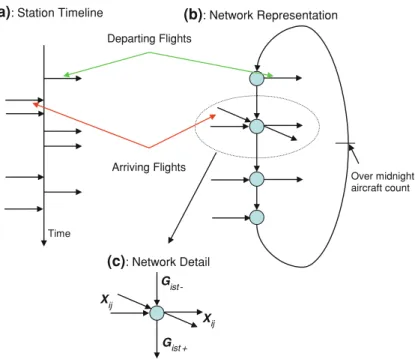
Typically, fleet assignment models pose the problem as a multi-commodity flow problem. For the fleet assignment problem, arcs represent the arrival and departure of flights and aircraft on the ground. The nodes define the specific time and station where these activities take place. Figure2.6 illustrates the basic timeline approach used by the fleet assignment model. Figure2.6a portrays the actual timeline of flights arriving and departing a single station. Figure2.6b pre-sents the node/arc representation of the timeline for the same station. Figure2.6c provides a detailed schematic of the decision variables that represent the selection of aircraft typeiassigned to flight legjand ground arcs flowing into a single node at timet and stationswithin the timeline.
Using this network representation, we formally develop the basic FAM pro-posed by Hane et al. (1995) using notation similar to that used by Lohatepanont (2001) and Smith and Johnson (2006).
2.5.2.1 Definition of Sets
S: set of stations or airports indexed bys.
J: set of flight legs indexed byj.
F: set of fleet types (e.g. S80, 737) indexed byi.
T: set of all departure and arrival events indexed byt.
Re(i): set of all flight legs for fleet typeicrossing the counting line (e.g. midnight) indexed byj.
IN(i,s,t): set of flight legs inbound to {i,s,t}.
OUT(i,s,t): set of flight legs outbound from {i,s,t}.
Gist
-Gist + Xij
(a): Station Timeline (b): Network Representation
(c): Network Detail Time Over midnight aircraft count Xij Departing Flights Arriving Flights
Fig. 2.6 Network representation of a typical FAM formulation.aStation timeline.bNetwork representation.cNetwork detail
2.5.2.2 Decision Variables
xij¼
1 if aircraft type i 2 F is assigned to schedule leg j 2 J;
0 otherwise :
Gistþ represents the number of aircraft on the ground for fleet type i2 F; at
stationss2 S;on the ground arc just following timet2 T:
Gist represents the number of aircraft on the ground for fleet type i2 F; at
stationss2 S;on the ground arc just prior to time t2 T:
2.5.2.3 Parameter Definitions
Rijrepresents the expected revenue associated with assigning aircraft typei2 Fto flight legj2 J and is a function of expected demand, spill and unit revenue per passenger.
Cijrepresents the expected costs associated with assigning aircraft typei2 F to flight legj2 J as a function of fixed, ownership and variable costs.
NPi represents the number of available aircraft of typei2 F:
2.5.2.4 Conventional Leg-Based FAM Formulation
max P¼X
j2J
X
i2F
ðRijCijÞxij ðObjective:Maximize ProfitÞ ð2:1Þ
subject to:
X
j2ReðiÞ
xijþX
s2S
Gis0 NPi 8i 2 F ðPlane CountÞ ð2:2Þ
GistGistþþ X j2INði;s;tÞ xij X j2OUTði;s;tÞ xij¼ 0 8i2F;s2S;t2T ðBalanceÞ ð2:3Þ X i2F xij¼1 8j 2 J ðCoverÞ ð2:4Þ
xij 2 f0; 1g 8i 2 F; 8j 2 J
Gisj0 8i2F; s2S; t2T ð2:5Þ
Constraints (2.2) represent resource constraints and states that the number of planes of each fleet typeicannot exceed the total number of planes available,NPi.
Constraints (2.3) represent the balance constraints stating that, at any station and time, the arrival of an aircraft must be matched by the departure of the aircraft. Aircraft can arrive at a station from another station or from the same station in the previous time event,t-1. The time events in this formulation represent an arrival or departure event or a combination of arrivals and departures at the station. Constraints (2.4) represent the cover constraints that stipulate each flight leg must be assigned a fleet type. Constraints (2.5) define the decision variable for assigning fleet typei to flight leg jas a binary variable and specify non-negativity for the ground arcs. Several references present overviews of the general leg-based FAM (see Abara1989; Subramanian et al.1994; Hane et al. 1995).
The conventional fleet assignment model described by Eqs.2.1–2.5is used for both long-term planning of the airline schedule and near-term finalization of the schedule fleet allocation. Depending on the carrier, this model can be used for long-term planning to fleet a typical daily schedule or a weekly schedule. Most U.S. based carriers tend to plan schedules based on a typical day while European and Asian carriers tend to focus on weekly schedules.
During the planning process, carriers will often need to reduce or expand their schedules to better match available capacity to demand during off seasons such as the fall and early winter or high demand seasons such as Christmas and New Year’s holidays. In these cases, airlines can use the FAM to help select and fleet flights that best contribute to the overall profitability of the schedule while drop-ping other flights that do not contribute. To reduce the schedule, airlines can run the FAM in ‘‘reduction mode’’ in which we relax the cover constraint described by Eq.2.4. Relaxing Eq.2.4as a less than or equal to constraint allows the model to drop flights that do not help maximize the overall profitability of the schedule.
Similarly, the relaxed version of the FAM can be used to expand the schedule to capture the need for more capacity during high demand seasons. To accomplish this, many airlines ‘‘overbuild’’ schedules to include more flights than they expect to operate. Using the overbuilt schedule as input, the airline then optimizes the schedule using the FAM in reduction mode to drop less desirable flights from the schedule.
In both cases mentioned above, the airline must add a number of operational constraints to the FAM to prevent undesirable results. Often these added con-straints place bounds on the number of frequencies allowed in any market and limit the number of flights dropped overall. This prevents the model from dropping out of markets entirely or radically reducing the resulting schedule in the name of expected profitability. One caveat that should be kept in mind involves the reve-nues and costs used to drive the objective function when using reduction mode. The FAM described by Eqs.2.1–2.5requires accurate reflections of the revenues and costs associated with each potential fleet/flight combination considered by the
model. These revenue and cost estimates are dependent on the original schedule used to forecast demand and passenger traffic. Relaxing the cover constraint (Eq.2.4) compromises the accuracy of these forecasts and the overall estimates for revenue and costs. Many carriers try to limit this undesirable impact by iteratively updating the forecasted revenues and costs to ensure more accurate results. However, this problem extends beyond schedule reductions. In fact, the revenues, costs and fleeting results can be influenced by the overall mix of local and con-necting passengers. As a result, several enhancements to the FAM have been proposed to incorporate the influence of connecting passengers and accurately reflect the change in revenues due to limited schedule reductions.
During the near-term planning process, the FAM can be used to finalize the overall fleeting (allocate sub-fleets), incorporate crew considerations into the final schedule and build transition schedules that bridge one seasonal schedule into the next. To build a transition schedule, an airline can formulate the FAM using the final fleet assignments from the two seasonal schedules as inputs and allow the model to optimize the fleet assignments to connect the two schedules. In addition, the FAM can be used to re-fleet portions of the schedule to better match overall demand to available capacity near the day of departure. We present an actual case study of this type of application near the end of the chapter.
As highlighted above, the major problem with the leg-FAM approach described by Eqs.2.1–2.5 is that it does not accurately incorporate the O&D marketing effects and expected passenger flows throughout the network. The fleet assignment process should account for multiple markets utilizing each leg of the schedule, multiple classes within each market, and network interactions caused by the various markets competing for space.
Several approaches to incorporating RM aspects into FAM have been investi-gated over the past 10 years to develop an Origin–Destination Passenger-based Fleet Assignment Model (ODFAM). These approaches have dealt with the size and non linearity of ODFAM through various decomposition approaches.
Farkas (1996) demonstrates that RM has a significant impact on traffic volume and mix and by ignoring these effects FAM can yield sub-optimal solutions. His analysis illustrated the necessity of modeling the effects of both network flow and stochastic demand to improve FAM performance. He concludes that incorporating RM directly into FAM is not practical. He proposes three approaches to this problem:
• Column generation. Where each column represents a complete fleeting solution. The master evaluates traffic and revenue, and ensures that allocations do not exceed capacity. The columns are generated using a multi-commodity formu-lation. Although no computational results are published Farkas states that the subproblem is relatively slow to solve (40 min) and is impractical for opera-tional use.
• Leg Class revenue management FAM. Since many airlines do not have full network control in their RM systems, Farkas investigates the impact of leg class revenue management control on FAM. He shows that for a typical airline fare
structure, the revenue function could be non-concave. This non-concavity makes this formulation unattractive in terms of computational efficiency.
• Decomposing the flight schedule into subnetworks between which there are limited or no leg-interactions. Fleeting solutions for each sub-network are generated, the traffic and revenue for each sub-network is evaluated with a Monte Carlo simulation. In the FAM formulation, each of the assignments for a subnetwork is represented by one meta-variable. By starting with a feasible leg-FAM solution, this approach should always produce improving solutions. No computational results are available.
Knicker (1998) and Barnhart et al. (2002) investigate the interactions between RM and FAM. In this work, the authors develop a Passenger Mix Model (PMM) that gives a schedule with known flight capacities and a set of passenger demands with known fare, and determines optimal traffic and revenue. PMM includes aspects of customer choice modeling and includes recapture (the probability that a customer who is spilled from one flight leg books on another of the same airline). PMM assumes that demand is deterministic and that the airline has complete knowledge and control of which passengers they accept. PMM could be formu-lated as a multi-commodity flow problem but due to the large number of passenger types and potential paths this approach is impractical. Kniker reduces the problem by using key-paths, the originally desired itinerary for each passenger. Alternate itineraries are necessary only when passengers are spilled from their preferred itinerary. The problem is solved using column generation, with each column representing passengers spilled from one itinerary and recaptured on another. Kniker formulates the stochastic version but does not present results.
Kniker combines PMM and FAM. The integrated problem, IFAM, is solvable but suffers from increased fractionality versus leg-FAM in which aggregate leg revenues and costs are used to reflect profitability of different fleets on a flight leg. He improves performance through coefficient reduction and additional cuts, but the MIP is still much more difficult to solve than the corresponding leg-FAM MIP. Kniker compares performance of various approaches using a Monte Carlo simu-lation model. By comparing models that capture the network effects assuming deterministic demand versus stochastic models that ignore network effects, he shows that if flow demand is at least 25% of the total demand, then capturing network effects is more important than capturing stochastic effects. Knicker does not formulate a version of FAM that addresses both stochastic demand and net-work effects.
Lohatepanont (2001) continues the analysis of IFAM. He investigates the sensitivity of IFAM to several of the simplifying assumptions in its formulation:
• Demand uncertainty. IFAM assumes that demand is fixed and known. The demands used in FAM are forecasts subject to random and systematic errors
• Imperfect control. PMM assumes that airlines have complete control over which passengers are accommodated
Through simulation analysis of IFAM and PMM Lohatepanont shows that while relaxing these assumptions, to make the models more realistic, reduces the benefit of IFAM versus leg-FAM, IFAM consistently outperforms FAM. Barnhart et al. (2002) provide an excellent recapitulation of Kniker and Lohatepanont’s work and the relationship between capacity assignments and RM passenger allo-cations in a deterministic setting. We present the model proposed by Barnhart et al. (2002) in the next section.
Erdmann et al. (1997) proposes a sequential approach to the itinerary FAM problem. They solve FAM and then the passenger mix problem. Kliewer (2000) proposes an approach that integrates FAM and RM using simulated annealing. Kliewer uses a neighborhood search strategy, starting with an initial feasible solution and looks for improving assignment swaps. He accepts or rejects new solutions based on a simulated annealing strategy. The revenue is evaluated with a deterministic passenger flow model.
The model proposed by Barnhart et al.2002 improves the conventional leg-based FAM by explicitly incorporating thenetworkandrecapture effectsinto the fleeting process. To better understand this motivation, consider the following example.
Network and Recapture Effects: An Illustrative Example
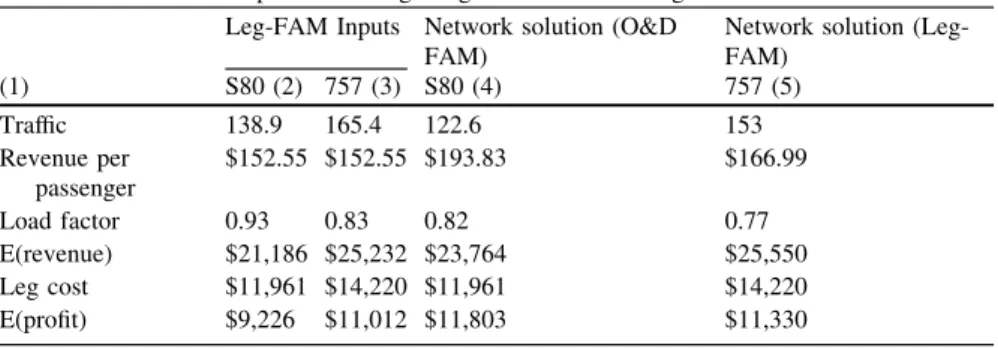
Consider a small airline network with two flight legs: Flight 001 ABQ-DFW and Flight 002 DFW-BOS. Table2.1shows demand and fare data in three OD markets ABQ-DFW, DFW-BOS and ABQ-BOS (connecting through DFW). If 100-seat aircraft is assigned to both flight legs in the network, the optimal revenue for the network of $41,875 is obtained by accommodating 75, 75 and 25 passengers from ABQ-DFW, DFW-BOS, and ABQ-BOS markets respectively.
In conventional FAM, flight legs are assumed to be independent; consequently, fares of connecting passengers have to be allocated to corresponding flight legs in the itineraries. Knicker (1998) experiments with a number of fare allocation schemes and shows that no single allocation scheme, which is applicable to all networks, exists. In this example, we use a simple ‘‘equal-fare’’ allocation, in which the connecting fare is divided equally among the flight legs making up the itinerary. Thus, in our example, the ABQ-BOS fare of $400 is equally divided and allocated to ABQ-DFW and DFW-BOS flights ($200 each). With this allocation,
Table 2.1 Itinerary demand information
Market Itinerary (sequence of flights) Number of passengers Average fare ABQ-DFW 001 75 $220 DFW-BOS 002 120 $225 ABQ-BOS 001–002 80 $400
the optimal leg-based revenue is obtained by maximizing the revenue on each flight independently. As a result, the optimal passenger mix is 75 and 25 pas-sengers from ABQ-DFW and ABQ-BOS markets respectively for Flight 001, and 100 passengers from DFW-BOS market alone for Flight 002. The optimal revenue is $44,000. Notice that the resulting optimal mix of passenger is infeasible because none of the ABQ-BOS passengers get on Flight 002, and thus the revenue of $44,000 is inaccurate and unachievable.
Alternatively, one can view this as leg-based FAM’s inability to calculatespill
consistently in the network. When the total passenger demand for a flight leg exceeds the capacity of that flight leg, some passengers are not accommodated or are spilled. In this example, with leg-based FAM, 55 ABQ-BOS passengers are spilled from Flight 001, but 80 ABQ-BOS passengers are spilled from Flight 002. On the other hand, with the optimal passenger mix given at the beginning of this example, 55 ABQ-DFW passengers are consistently spilled from both legs.
Next, we introduce the concept of recapture. Normally, spilled passengers are either (1) lost to the airline (that is, they choose to travel on competing airlines or choose not to travel by air) or (2)recapturedon alternative flights in the network of the original airline. These recaptured passengers generaterecaptured revenue
for the airline on alternative flights. Most leg-based fleet assignment models ignore totally these recaptured revenues in their estimation of flight-leg revenues because inconsistent spills cannot possibly lead to accurate recapture estimates.
In conclusion, leg-based FAM cannot estimate flight-leg revenues accurately because it assumes flight-leg independency. Specifically, the inaccuracy is a result of (1) the inconsistent estimates of spills due to the network effect and, conse-quently, (2) the inaccurate estimates of (possibly significant) recapture revenues due to therecapture effect.
Further, this example demonstrates how decisions made independently for each flight leg are incorrect and suboptimal. To get an accurate estimate of passenger revenue, one needs to take a holistic look at the entire network.
Passenger Mix Model
As the example above shows, a leg-based view of the network does not accurately capture the network effects due to O&D passenger flows and recapture. We need a tool that can estimate the network revenue more accurately. Specifically, we need a tool that can estimate spill consistently throughout the network and allow recaptured revenue to be estimated systematically. Knicker (1998) proposes the PMM for this purpose. The objective of PMM is to find the optimal itinerary-based mix of passengers that maximizes the total revenue (including recaptured revenue) or, equivalently, minimizes the total spill cost, the revenue loss due to spilled passengers. PMM is formulated as follows:
Min X p2P X r2P farepbrpfarer tpr ð2:6Þ Subject to:X p2P X r2P dpitrpX r2P X p2P dpibprtprQiCAPi 8i2L ð2:7Þ X r2P trpDp 8p2P ð2:8Þ tpr0 8p;r2P: ð2:9Þ
This formulation utilizes a special set of variables (keypath variablestpr), first
proposed by Barnhart et al. (1995), to enhance model solution. Specifically, the model a priori assigns passengers to their desired itineraries; next, if the capacities on some flights are insufficient, the model finds an optimal way to spill passengers off from these flights such that the totalspill cost(the revenue loss due to spilled passengers) is minimized. This model incorporates recaptures using a set of Quantitative Service Index (QSI) based parameters called recapture rates, bpr,
which is defined as the recapture rate from itinerarypto itineraryror the fraction of passengers spilled from itinerary p that the airline succeeds in redirecting to itineraryr.
LetPbe the set of all itineraries andLbe the set of all flight legs. The decision variable, tp
r
, is the number of passengers who are redirected from their desired itinerarypto an alternative itineraryr. The parameter farepdenotes the averaged
fare for itineraryp. The objective function (Eq.2.6) minimizes the total spill cost
P p2P P r2P fareptrp !
less the recaptured revenue P
p2P P r2P br pfarertpr ! . Con-straints (2.7) ensure that the total number of passengers for each flight legi(which equals to the original passengers desiring this flight, Qi, less the total passengers
spilled from this flight,P
p2P
P
r2P
dpitrp;plus the total passengers recaptured from other flights,P
r2P
P
p2P
dpibp
rtrp) does not exceed the capacity of that flight,CAPi.dipequals 1
if itineraryputilizes flight legi, 0 otherwise. Constraints (2.8) and (2.9) ensure the number of spilled passengers for each itinerary does not exceed the demand for that itinerary and is not less than zero.
PMM is a large-scale LP model that requires specialized solution algorithm. Knicker (1998) proposes a column and row generation-based algorithm for the model. Specifically, only a small set of variables is included in the original master problem and, as the algorithm progresses, more columns (variables redirecting passengers to alternative itineraries) are generated as necessary. Notice also that in the optimal solution most of Constraints (2.8) are not binding because most of the passengers are traveling on their desired (keypath) itineraries. Thus, Constraints (2.8) can be initially omitted and subsequently generated back in as necessary.
Itinerary-Based Fleet Assignment Model
The Itinerary-Based Fleet Assignment Model (IFAM) is the integration of the PMM and the leg-based FAM. The IFAM formulation is:
Min X k2K X i2L ck;ifk;iþ X p2P X r2P farepbrpfarer tpr ð2:10Þ Subject to:X k2K fk;i¼1 8i2L ð2:11Þ yk;o;tþ X i2INðk;o;tÞ fk;iyk;o;tþþ X i2OUTðk;o;tÞ fk;i¼0 8k;o;t2N ð2:12Þ X o2A yk;o;tmþ X i2CLðkÞ fk;iNk 8k2K ð2:13Þ X k2K SEATkfk;iþ X p2P X r2P dpit r p X r2P X p2P dpib p rt p rQi 8i2L ð2:14Þ X r2P trpDp 8p2P ð2:15Þ fk;i2f0;1g 8k2K;8i2L ð2:16Þ yk;o;t0 8k;o;t2N ð2:17Þ tpr0 8p;r2P: ð2:18Þ
The objective function (Eq.2.10) minimizes the total operating cost (P
k2K
P
i2L
ck;ifk;i)
and the total spill (less recapture) cost P
p2P P r2P farepbrpfarer trp ! . Constraints (2.11)–(2.13) are original FAM constraints—coverage, balance and count con-straints, respectively. Constraints (2.14) are capacity constraints, which dictate that for a given flight legithe capacity of the chosen assignment (P
k2K
SEATkfk;i) must
exceed the total traffic QiP
p2P P r2P dpitrpþ P r2P P p2P dpibprt p r ! . Constraints (2.15) guarantee that no spills exceed demands. Constraints (2.17) ensure binary selectivity. And finally Constraints (2.17)–(2.18) ensure non-negativity.
Because IFAM is an integration of two large-scale models, Barnhart et al. (2002) propose a column and row generation-based solution algorithm for solving IFAM. Specifically, the column and row generations are applied to the PMM part of the model, that is, to the traffic variables (tpr) and demand constraints
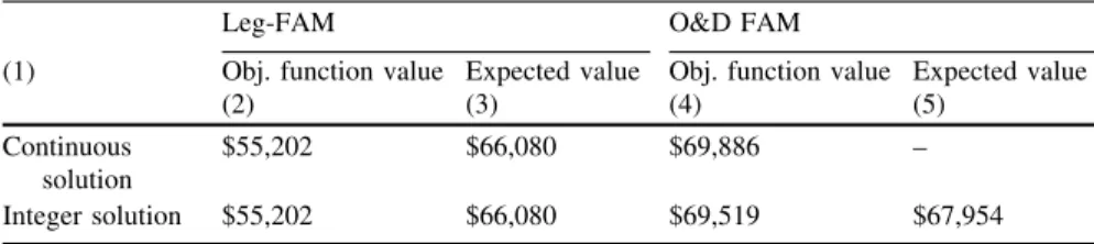
Barnhart et al. (2002) test the model and algorithm on actual large-scale data set of a major U.S. airline. Their results indicate significant savings from the optimal assignment of aircraft types to flight legs, taking into account network and recapture effects. Further, they present experiments to validate IFAM’s three key assumptions/parameters, namely, (1) deterministic demand, (2) recapture rate and (3) optimal control of passenger mix through PMM. Their findings indicate that (1) in a simulation test using stochastic demand generator, IFAM fleeting decisions consistently outperform FAM fleeting decisions, (2) IFAM fleeting decisions are not particularly sensitive to a reasonable range of recapture rates and (3) in a simulation test where suboptimal control of passenger mix is simulated, IFAM fleeting decisions again consistently outperform FAM decisions. For detailed information and discussion, readers are referred to Barnhart et al. (2002).
Another approach for incorporating both network effects and the stochastic nature of demand first proposed by Jacobs et al. (1999,2000,2008) uses revenue management controls to drive the fleeting process. This model uses a Benders decomposition approach to integrate the FAM model with a stochastic O&D Revenue Management model. We refer to this approach as O&D FAM. The revenue associated with any FAM solution depends on the capacity assignment for all flight legs. Given an assignment solution, the O&D revenue is estimated by the O&D RM sub-problem. The revenue function for the entire network is approxi-mated in the master problem (FAM) using a series of Benders cuts. Each cut improves the accuracy of the revenue approximation in the master FAM problem. Once a specified accuracy is achieved in the relaxed master problem, the assignment variables are changed to integer variables and the MIP is solved.
This approach is appealing because it addresses both passenger flows within the network and demand uncertainty. It also provides a method of incorporating the passenger mix optimization model used for revenue management directly into the fleet assignment process.
Typically, airlines estimate the expected revenue for each fleet-flight combi-nation using a proportional spill model (Swan 1983) and an average fare per passenger. This process applies a spill model to the total demand for each leg in the schedule individually. As a result, the leg-based revenue and profit estimates cannot capture the effects of network flow on the traffic of individual legs. Using this formulation, the total revenue for each leg in the schedule reflects an inde-pendent point estimate of the revenue function. This leads to errors in estimating the expected traffic and revenue for each leg in the schedule.
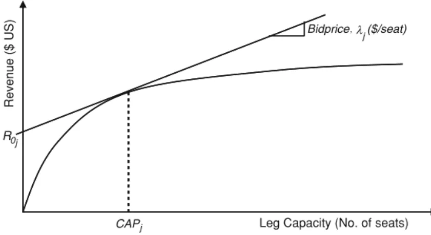
In reality, the revenue function accounts for the cumulative effect of all market classes flowing over leg j as a function of its capacity and incorporates the interaction between all the legs in the schedule. The revenue function is actually a concave function with respect to leg capacity, CAPj, resulting from O&D network
flow. Figure2.7 presents an illustrative example of the revenue function for a single leg in the network.
Network flow or O&D yield management (O&D YM) solutions yield a set of bidprices for each leg which represents the dual value of the O&D YM capacity constraint and equals the slope of the revenue function at a given leg capacity,
CAPj(Fig.2.3). This slope can be used to define a linear approximation and upper
bound to the revenue function. Mathematically, this upper bound is expressed as:
R0jþkjCAPjRðCAPjÞ ð2:19Þ
whereR0jrepresents the right-hand side of the linear approximation to the revenue function and RðCAPjÞ equals the total revenue as a function of the capacity of
legj, CAPj.kj defines the marginal value of an extra seat on legj (the bidprice)
resulting from the O&D yield management. Mathematically, the bidprice for leg
jis defined by:
kj¼oRðCAPjÞ
oCAPj
ð2:20Þ
In practical terms, the bidprice represents the minimum acceptable price of a seat. More importantly, the bidprice represents the change in the total system revenue due to a unit change in the capacity of leg j. Therefore, the bidprice captures the cumulative effects of the market classes flowing over leg j and the interactions between legjand the other legs in the network. Please see Appendix A for a complete formulation and review of the O&D Yield Management (O&D YM) model formulation.
For any solution of FAM and a corresponding set of bidprices, the total revenue for the schedule is the sum of the revenues realized on each leg. Summing over all the legs in the network yields the following upper bound on the total revenue (RTotal): X j2J R0jvþ X j2J kjvCAPjvRTotal 8v 2V ð2:21Þ Rev e nue ($ U S )
Leg Capacity (No. of seats) CAPj
j Bidprice, ($/seat)
R0j
where v is the index in the set V for a specific FAM and YM solution. This relationship represents a Bender’s cut (Parker and Rardin1988; Nemhauser and Wolsey1988; Bradley et al.1977) and defines an overall upper bound on the total revenue for the schedule as a function of network flow results. Therefore, the overall revenue used in FAM is limited by a function of O&D passenger flow resulting from the O&D YM process.
Constraints (2.21) relate the FAM to the network flow model. This relationship allows decomposition of the O&D FAM model into two separate but related problems: (1) a linear fleet assignment model and (2) a nonlinear network flow model. Separately, each of these models can be solved using conventional IP or NLP methods. Using Constraints (2.21), the general FAM is modified to include O&D effects. The resultinglinearFAM used by O&D FAM is defined as:
Linear FAM Formulation
max P¼RTotalCTotal ðObjective:Maximize ProfitÞ ð2:22Þ
subject to:
X j2ReðiÞ
xijþX
s2S
Gis0NPi 8i 2 F ðPlane CountÞ ð2:2Þ
GistGistþþ X j2INði;s;tÞ xij X j2OUTði;s;tÞ xij¼0 8i2F;s2S;t2T ðBalanceÞ ð2:3Þ X i2F xij¼1 8j 2 J ðCoverÞ ð2:4Þ X j2J R0jvþ X j2J kjv X i2F CAPijxij ! RTotal0 8v 2V ðRevenueÞ ð2:23Þ CTotal X j2J X i2F Cijxij¼0 ðCostÞ ð2:24Þ xij 2 f0; 1g 8i 2 F; 8j 2 J Gisj0 8i2F; s2S; t2T ð2:5Þ
For this formulation, the objective function is modified and two new constraints are added. Constraints (2.23) represent a variation of Constraints (2.21) and allows for the incorporation of the original binary decision variable,xij. Constraint (2.24)
simply redefines the total cost of the fleet assignment as a constraint. O&D FAM explicitly incorporates network effects by utilizing the bidprices provided by