Towards easy and efficient processing of ultra-high resolution brain images

TOWARDS EASY AND EFFICIENT PROCESSING OF

ULTRA-HIGH RESOLUTION BRAIN IMAGES

Valerie Hayot-Sasson

A thesis in

The Department of

Software Engineering and Computer Science

Presented in Partial Fulfillment of the Requirements For the Degree of Master of Computer Science

Concordia University Montréal, Québec, Canada

September 2017

Concordia University

School of Graduate Studies

This is to certify that the thesis prepared

By: Valerie Hayot-Sasson

Entitled: Towards easy and efficient processing of ultra-high resolution brain images

and submitted in partial fulfillment of the requirements for the degree of

Master of Computer Science

complies with the regulations of this University and meets the accepted standards with respect to originality and quality.

Signed by the final examining commitee:

Chair Dr. Tse-Hsun Chen Examiner Dr. Marta Kersten-Oertel Examiner Dr. Thomas Fevens Supervisor Dr. Tristan Glatard Approved

Chair of Department or Graduate Program Director

20

Amir Asif, Dean

Abstract

Towards easy and efficient processing of ultra-high resolution brain images

Valerie Hayot-Sasson

Ultra-high resolution 3D brain imaging is of great importance to the field of neuroscience as it provides a deep insight into brain anatomy and function. Such images may range between a few 100 gigabytes to terabytes in size and do not typically fit into computer memory. Lack of accessibility to the processing of these images is a threat to open science. This thesis aims to design a web system that will handle the storage and processing of ultra-high resolution neuroimaging data.

The system architecture uses technologies such as Hadoop Distributed File System and Apache Spark. For the seamless integration neuroimaging pipelines into our system, we adopted NIfTI as our distributed data format and require that all neuroimaging pipelines be described in common formats such as Boutiques or BIDS.

The large images are split into chunks, and also, recreated from the chunks. The effects of 2D slices and 3D blocks are investigated. Different algorithms to minimize number of seeks were designed and implemented. Results indicate that clustered reading of blocks achieves a significant reduction in processing time, and partitioning data into slices is most effective.

The scalability of processing large images with Spark using a simple non-containerized and containerized pipeline was investigated. It was found that processing time of both algorithms scale well. As data may need to be written to and read from disk for containerized pipeline processing, the speedup provided by Spark’s in-memory computing was also investigated. In-memory computing was found to provide significant speedup, however, this speedup may be less significant in more compute-intensive pipelines.

Acknowledgments

I would like to thank my supervisor Dr. Tristan Glatard for his support throughout the thesis. This thesis would not have been possible without the guidance of such a exceptional supervisor.

I would also like to thank my wonderful friends Anna, Lili, Madeleine, Alex, Danna and Lara, for sending me endless messages of encouragement throughout the process, as well as my family, for always being there for me.

Contents

List of Figures vii

List of Tables viii

1 Introduction 1

1.1 Background . . . 1

1.2 Goals and Contributions . . . 2

2 Tools used and related works 3 2.1 Introduction . . . 3

2.2 Big Data Infrastructure . . . 3

2.2.1 Hadoop Distributed File System . . . 4

2.2.2 Apache Spark . . . 5

2.2.3 Container images . . . 7

2.2.4 Containerized data-processing pipelines . . . 7

2.3 Image Formats and I/O libraries for large images . . . 8

2.3.1 NIfTI . . . 9

2.3.2 MINC 2.0 . . . 9

2.3.3 NiBabel . . . 10

2.4 Existing systems for large imaging data . . . 11

2.4.1 NeuroData Web Services . . . 11

2.4.2 CBRAIN . . . 11

2.4.3 Processing of large neuro-imaging data sets with Apache Spark . . . 11

3 A system to process ultra-high resolution 3D brain images 13 3.1 Introduction . . . 13

3.3 File types . . . 14

3.4 Partitioning and merging of data . . . 15

3.5 Running pipelines . . . 16

3.6 Describing pipelines . . . 17

4 Splitting and merging 18 4.1 Introduction . . . 18 4.2 Disk model . . . 19 4.3 Notations . . . 19 4.4 Algorithms . . . 20 4.4.1 Slabs vs blocks . . . 20 4.4.2 Buffered slabs. . . 21

4.4.3 Buffered blocks: Cluster reads . . . 22

4.5 Implementation . . . 25 4.6 Experiments . . . 25 4.6.1 Data . . . 25 4.6.2 Hardware . . . 26 4.6.3 Execution conditions . . . 26 4.7 Results . . . 26 4.7.1 Conclusion . . . 28 5 Pipelining framework 30 5.1 Introduction . . . 30

5.1.1 Describing neuroimaging pipelines in Spark. . . 30

5.1.2 Hardware . . . 31

5.1.3 Data . . . 31

5.2 Effects of parallelization on neuroimaging pipelines . . . 31

5.2.1 Histogram computation. . . 31 5.2.2 Containerized pipeline . . . 33 5.3 In-memory computing . . . 34 5.3.1 Conclusion . . . 35 6 Conclusion 36 Bibliography 40

List of Figures

1 System architecture diagram . . . 15

2 Example of an image index file . . . 16

3 Split and merge notations . . . 20

4 Buffer used in cluster reads . . . 20

5 Memory-load configurations in cluster reads . . . 23

6 Configurations that increase number of seeks per memory-load . . . 23

7 Number of seeks for all algorithms . . . 27

8 Breakdown of total merge times . . . 28

9 Average histogram computation times . . . 32

10 Containerized binarization pipeline processing times . . . 34

11 Comparison of total processing times between Spark’s in-memory computing and intermediary I/O . . . 35

List of Tables

Chapter 1

Introduction

The demand for systems that can support the processing of large images has increased in many scientific fields with the advancement of technologies that enable high resolution imaging. Such images range from a few hundred gigabytes to terabytes in size. As a result of their size, the images may not fit into memory and will likely result in lengthy processing times, therefore, access to hardware that can support these images is imperative. In addition, adequate knowledge of how to process such large volumes of data is necessary in order to be able to process images in a reasonable amount of time. The lack of accessibility to the processing of the such images threatens open-science by restricting analysis capabilities to a few. This thesis will focus on designing a web system to easily and efficiently process ultra-high resolution 3D brain images.

1.1

Background

High-resolution brain imaging technologies have emerged in recent years to improve understanding of the brain [1][2]. This thesis will examine the processing of BigBrain as a use case for the processing of high-resolution 3D brain images. BigBrain is an ultra-high resolution 3D human brain model, and is freely available online at various resolutions [3]. At its highest-resolution, 20µm isotropic voxels, the total size of the BigBrain image is 1TB. An updated version of BigBrain at a resolution of 1x1x20µm is planned to be released shortly, which would increase the data volume to 100TB. Other examples of medical imaging modalities which generate high-resolution images include electron microscopic (EM) imaging [4] and micro-computed tomography (microCT) [5].

1.2

Goals and Contributions

There is a need for a system that enables users to efficiently process large high-resolution and ultra-high resolution brain images. The system must be easy to use, ensure that memory consumption is controlled and processing time remains tractable. The existence of such a system would benefit open-science by making the processing and storing of large high-resolution brain images accessible to everyone.

The goal of this thesis is to contribute to the development of such a system by:

• Designing the overall architecture of the system, and

• Implementing the backend of the system

To effectively process such large images, a parallelization framework and distributed file system is needed. We have selected Apache Spark [6] as our system’s parallelization framework and the Hadoop Distributed File System (HDFS) [7] for file storage. The image data needs to be split into smaller chunks for parallel processing and may eventually be merged back for processing by other pipelines or reduced for output delivery. The splitting and merging scheme, as well as the algorithm selected can have great impacts on processing times. The contribution that this thesis has made towards the parallelization framework include:

• Finding effective algorithms to split and merge 3D imaging data given arbitrary splitting schemes.

• Designing and implementing a pipelining framework to process such high-resolution images, based on existing tools.

Our system will contribute to Open Science by making the processing of high-resolution imaging accessible to everyone. The code used to implement the system will also be publicly available through a GitHub repository.

The thesis will be broken into four chapters. Chapter2will examine the tools to be used in our system in addition to related works. Chapter3will focus on the system’s design and architecture. Chapter 4 will present new split and merge algorithms for high-resolution 3D images. Lastly, Chapter5will present the pipelining framework through various use cases.

Chapter 2

Tools used and related works

2.1

Introduction

In order to be able to design a system that is capable of processing larges images, a parallelization framework and distributed filesystem were selected. To support the processing of the images through existing neuroimaging pipelines, the pipelines were executed within a container – an operating system (OS) virtualization environment containing all necessary libraries. Since we are supporting the integration of existing neuroimaging pipelines into our system, the distributed file format will consist of popular neuroimaging file formats. To determine the most suitable file type for our system to initially support, we investigated different neuroimaging file types and associated libraries that support reading and writing of such file types.

This chapter will review the various pre-existing elements we will be incorporating into our system as well as investigate similar systems. Section 2.2 will look at the infrastructure of the system. Section2.3will discuss different neuroimaging file formats and the existing libraries that can read and write these formats. Lastly, Section2.4 will review similar systems that have been implemented.

2.2

Big Data Infrastructure

To parallelize the processing of the ultra-high resolution images, it is necessary to use a distributed file system to reduce data transfer time and have an efficient parallelization framework. We propose the use the of the Hadoop Distributed File System (HDFS) as our system’s distributed file system, and Apache Spark as our parallelization framework. Both of these technologies have been designed to work with large amounts of data and have been applied successfully to similar contexts in other

domains such as satellite imagery [8].

2.2.1

Hadoop Distributed File System

The Hadoop Distributed File System (HDFS) is a distributed file system designed to support applications running large datasets, typically supporting file sizes that range from gigabytes to terabytes [7]. The system prioritizes high-throughput of data over low latency, and its write-once-read-many data-access model enables such high-throughput data access. HDFS is a fault-tolerant system that uses data-replication to maintain performance during failures. In order to accommodate data-locality, HDFS provides interfaces for applications to move closer to where the data is located.

Architecture

The architecture in HDFS is that of master-slave. There is one master, the NameNode, located in a dedicated machine, and one to many slaves, the DataNodes, typically each located in a separate node in a cluster. The role of the NameNode is to manage the filesystem namespaces and regulate user access to files. It can execute typical file system operations such as opening and closing a file as well as renaming files and directories.

As HDFS typically handles large files, these files need to be partitioned into blocks and distributed to the DataNodes. The NameNode is responsible for splitting these files into, for instance, 128MB, and mapping them to the DataNodes. In addition, the NameNode makes all decisions related to replication of blocks.

DataNodes, on the other hand, manage the storage of the nodes in which they run on. They store their data within their local filesystem and have no knowledge of HDFS files. The operations that a DataNode can perform include: block creation, deletion, and replication of the data as instructed by the NameNode. In order to broadcast its proper functioning to the NameNode, the DataNode periodically sends the NameNode a heartbeat signal. The DataNode also sends a BlockReport back to the NameNode to advise it of the blocks stored within the DataNode.

Fault-Tolerance through Replication

To ensure the system remains fault-tolerant, data from the blocks must be replicated across the nodes. By default, the replication factor of the blocks in HDFS is 3, however, a different replication factor can be specified during file creation and be modified at a later time. Since HDFS may run on cluster computers containing many racks, it is important that inter-rack communication is limited

as it is slower than intra-rack communication. However, it is also important to place replicas across different racks, as racks may fail. In the case of the default replication factor, this is achieved by replicating the data across two different DataNodes located on the same local rack and replicating the data once on a DataNode located on a remote rack.

2.2.2

Apache Spark

In addition to having a scalable, distributed filesystem, the proposed system also requires a par-allelization framework that can run on large-data and is compatible with the filesystem (HDFS). Apache Spark (Spark) is such a parallelization framework [6]. Spark is designed for the handling of large-scale data intensive applications. It is written in Scala for the Java Virtual Machine (JVM), however, there are other, albeit less comprehensive, implementations for programming languages such as Python. Spark is much faster in processing in comparison to its predecessor, Hadoop MapReduce, as data is kept in memory during acyclic data flows and does not need to be reread from disk. In order to execute Spark, users implement a high-level control flow within a driver application using Spark’s abstractions. For scheduling Spark tasks, Spark offers its own standalone scheduler, and is also compatible for use with Yet Another Resource Negotiator (YARN) [9] and Apache Mesos [10].

The main parallel programming abstraction in Spark is the Resilient Distributed Dataset (RDD). The RDD is a read-only collection of objects partitioned across various machines. Spark is able to ensure fault-tolerance through RDDs as they can be rebuilt if a partition is lost. Acyclic data flow computations are facilitated by RDDs as users can cache them in memory and reuse them in other MapReduce-like parallel operations. RDDs can be constructed in four ways: 1) from an existing file located in a shared filesystem (ex. HDFS), 2) by parallelizing a Scala collection (ex. array) in the driver program, 3) by applying a transformation to an already existing RDD using map or filter transformation, 4) or by changing the persistence of a currently existing RDD through caching or by writing the RDD to file.

Other abstractions in Spark include the parallel transformations and actions that can be executed on the RDDs. An example of a common transformation is map. map takes each element in the RDD, applies a function to it, and returns a transformed version of the original RDD. Frequently used actions include: reduce, collect, foreach. reduce applies an associative function to combine the dataset elements and produce a result at the driver program. collect will simply send all elements to the driver program. foreachwill pass each dataset element to a user-defined function. Since Spark uses lazy-evaluation, transformations will only be evaluated after a call to an action.

Spark also contains shared variables, such as broadcast variables and accumulators. Shared variables are variables which are used by multiple nodes and are not limited to the scope in which they were created. Broadcast variables allow large read-only files to be copied only once to each worker node rather than copying it at each function execution. Accumulators, however, are variables which can only be added to by worker nodes using an associative operation and are only readable by the driver.

Although other parallelization frameworks do exist, Spark is ideal in our context. Features of Spark that make it desirable to our system, in addition to data-locality and in-memory computing, include ease of use and compatibility with commodity hardware. These features are important to have in an open-science context as it permits those who are not programmers by trade to easily create parallelizable pipelines, and allows them to execute it on affordable hardware.

Listing 2.1 shows an example of how to code with PySpark - the Python implementation of Spark.

Listing 2.1: Example of a PySpark pipeline to count number of voxels in an image

# Example of a PySpark pipeline

# Count number of voxels in NIfTI-1 image

import numpy as np

from pyspark import SparkContext, SparkConf

# initialize the Spark context

conf = SparkConf().setAppName("example app") sc = SparkContext(conf=conf)

# create RDD from binary files in folder imgRDD = sc.binaryFiles("folder/example")

# extract number of elements in image

# and return new RDD where all element keys are 1 and values # represent the number of voxels in image

# note: x represents image key-value pair. # x[1] contains image binary data

# print number of voxels in image to screen

# reduceByKey function combines all elements of the same key by # summing their counts

print dataRDD.reduceByKey(lambda x,y : (x + y)).collect()

2.2.3

Container images

Existing neuroimaging pipelines, such as, the FreeSurfer Software Suite (FreeSurfer) [11], FMRIB Software Library (FSL) [12] and Statistical Parametric Mapping (SPM) [13], represent decades of effort by the community. For this reason, we want these pipelines to be accessible to the system. Such neuroimaging pipelines are complex and may have many dependencies that need to be accessed by our system. To address this, we will use container images.

Container images are executable packages that contain complete OS distributions except the kernel. They are lighter than Virtual Machines (VM) as containers perform virtualization at the operating system (OS) level, unlike a VM’s hardware-level virtualization which comes with performance penalties [14]. Containers allow for user-defined development stacks as they provide a portable platform for the user’s custom libraries, build environments, and sometimes entire operating systems to run on.

Many container technologies exist, such as OpenVz [14], BSD jails [15], LXC [16], and Docker [17]. Docker is currently the most popular container technology. While Docker is very good at meeting the industry’s need for containers, it fails to meet the security requirements required in scientific high-performance computing (HPC) environments. Within a Docker container, users can gain elevated privileges in the underlying system, as all container users are root users. This is a problem in HPC environments as typical users are restricted users and should not gain root access. To address the security flaw imposed by Docker containers in HPC environments, Singularity containers were created [18]. Singularity containers provide all the functionality of a Docker container, but have the added restriction of maintaining the underlying system’s user privileges within the container, and cannot be granted elevated privileges. As such, Singularity containers can be created by the users in a local environment where the users have root privileges. A Singularity container should not require root privileges for execution.

2.2.4

Containerized data-processing pipelines

The user-defined pipelines, stored within Docker containers, will be executed by the system. To facilitate the execution of these user-defined apps within the system, we require that the application

meet the requirements of a BIDS (Brain Imaging Dataset Standard) App [19] or that it be made into a Boutiques App [20] through the incorporation of a Boutiques tool descriptor.

In order to meet the requirements of a BIDS App, the user-defined neuroimaging pipeline, stored within a Docker container that can be accessed through DockerHub, must contain a wrapper that is formatted to accept a certain type and number of command-line arguments and run execute on BIDS conformant datasets. As it is very likely that the pipeline will be executed in an HPC environment, and therefore deployed using Singularity, the pipelines within the containers must not require any form of elevated security in order to execute. As well, environment variables will need to be specified within the Dockerfile rather than within the container’s root config files and the application cannot write outside of /tmp, the user’s home directory, or the specified output directory.

The required command-line arguments for a BIDS app include: input_dataset,output _folder and analysis_level. input_dataset represents the path to a read-only BIDS dataset, output_folder is the path to the folder where the output will be stored, whereas, analysis_levelrepresents that stage of analysis to be performed. Additionally, theanalysis _levelmay also be limited to a subset of participants within the dataset. In this case, the argument participant_labelmay also be included.

A Boutiques app is similar to that of a BIDS app in that it facilitates integration and execution of processing pipelines into systems using lightweight Docker containers. However, unlike a BIDS app which must conform to a strict command-line interface, a Boutiques app is not limited to specific arguments. A Boutiques tool descriptor, written in JSON, may define any command-line arguments required by the application. Thus, a Boutiques app is capable of being created from an existing application without any modification to the command-line arguments of the original application.

2.3

Image Formats and I/O libraries for large images

Our system intends to be compatible with commonly-used neuroimaging pipelines. Such pipelines have been instrumented to work with specific neuroimaging file formats, and would need to be altered to be able to support a new distributed file format. There are several files file formats for neuroimaging including NIfTI-1 [21], MINC 2.0 [22] and DICOM [23]. NIfTI-1and MINC 2.0 are the most ubiquitous file format in neuroscience. DICOM, however, is a popular file format in the industrial neuroscience sector. As we want to allow for easy integration of neuroimaging pipelines into the system, we will focus on adapting our system to allow for the distributed processing of

well-supported and widely accessible file formats: MINC 2.0 and NIFTI.

2.3.1

NIfTI

NIfTI-1 was designed as an extension of the popular ANALYZETM 7.5 file format [21]. The NIfTI-1 header re-purposed unused fields from the ANALYZETM 7.5 file format to fields which are desirable to functional magnetic resonance imaging (f-MRI) analysis. The NIfTI file format remains compatible with non-NIfTI aware ANALYZETM7.5 software.

Similarly to the ANALYZETM7.5 file format, the NIfTI-1 image consists of two components: header (.hdr) and image data (.img). These components can also be merged into a single.nii file. The.hdror header component is, like the data, stored in binary and a maximum of 348 bytes in size. To differentiate the NIfTI file format from the ANALYZETM 7.5 file format, the last 4 bytes of the header are dedicated to the NIfTI-1 magic number. Should the NIfTI-1 magic number be missing from the header, a NIfTI-aware software will treat the image as an ANALYZETM 7.5 image. The NIfTI format also accepts an extension to the header, which is located immediately after the 348 byte header and its size is denoted by the voxel offset property of the header.

Data representation in NIfTI is in column-major order. In other words, for an image of dimensions (i, j, k), i is the fastest changing dimension, followed by dimension j, followed by dimension k. The maximum size of the data is limited by the dimension information provided in the header. This dimensions listed in the header can be a maximum of 16-bits signed integer in size (i.e. a maximum of 32767 in size per dimension). To overcome the image dimension limitation, the NIfTI-2 file format was created. It is an extension to the NIfTI-1 file format that has a 540 byte header instead of a 352 byte header. This larger header permits the image dimensions to go up to a maximum of a 64-bit integer.

2.3.2

MINC 2.0

An alternative to the simple NIfTI format, in which data is stored in a linear fashion, is the MINC 2.0 format [22]. Unlike its predecessor (MINC), MINC 2.0 utilises the HDF5 to render its contents fully extensible and hierarchical. The incorporation of the HDF5 library also provides the added feature of internal compression. Like NIfTI-2, MINC 2.0 supports 64-bit data. MINC 2.0 also supports high-dimensionality and irregularly-shaped dimensions.

Data within the MINC 2.0 file format is hierarchical, consisting of groups encapsulating sub-groups, similar to that of a file system. The root group of the image isminc 2.0. In it is stored the metadata in addition to the following subgroups: image,infoanddimensions. Image data

is stored within theimage subgroup, and details on image orientation, coordinates, size, etc,. is stored within the dimensionssubgroup. Since it is hierarchical in nature, it is possible to store multiple resolutions of an image within a single file. Different resolutions are to be stored within a subgroup of theimagegroup.

Unlike NIfTI, data representation within the MINC 2.0 file format is in row-major. In other words, for given dimensions (i, j, k), dimension k increases most rapidly, followed by j, which is followed by i.

Image data in MINC 2.0 may be partitioned into limited-sized "chunks". This permits lossless compression of the chunks and allows for true random-access in compressed volumes. This is a desirable feature for our system as we want to be able to decompress chunks of an image at a time-which is not guaranteed with image formats such as NIfTI. Although, NIfTI can be extended to support access reading of compressed data, it is not currently possible to achieve random-access writing of data [24].

2.3.3

NiBabel

NiBabel is a popular Python library used for the reading and writing of various neurological imaging file formats, including NIfTI-1, NIfTI-2 and MINC 2.0 [25].

A NiBabel object consists of three parts: an image header, an a 4x4 affine matrix mapping voxel coordinates to Right, Anterior, Superior positive (RAS+) world coordinate space, and image data. In order for a NiBabel object to be created, it simply requires an array containing image data and the affine matrix.

Should an image be loaded from disk, the image array will not necessarily be loaded into memory immediately. The image, referred to a as aproxyimage, will contain adataobjproperty that can fetch the data from the disk. To access array data, the get_data() object needs to be called. For the instance in which only a subset of the data is required, or the entirety of the data does not fit into memory, array proxy slicing can be used. This is a useful feature, particularly for our system, where the images are too large to fit in their entirety into memory. With array proxy slicing, we can select as much data that can fit into memory for processing, at a time

2.4

Existing systems for large imaging data

2.4.1

NeuroData Web Services

The NeuroData Web Services (NDstore), formerly know as The Open Connectome Data Cluster, is a scalable database cluster designed for spatial analysis and visualization of high-throughput neuroimaging data [26]. The database cluster allows for the distributed storage of image data and their annotations, but does not permit the user to apply a custom pipeline to the image data stored within the database. Image data uploaded to the cluster is converted to the database cluster’s custom database structure. Image data is partitioned into cuboids assigned with an index using a Morton-order space-filling curve [27] to ensure that cuboids are ordered in a way such that the data remains contiguous. Annotation data is also stored in cuboids. A copy of the image data is stored into 2D tile stacks for web-visualization.

2.4.2

CBRAIN

The Canadian Brain Imaging Reasearch platform (CBRAIN) is a web-based collaborative research platform designed for distributed storing, processing and visualization of large-scale neuroimaging data [28]. The CBRAIN platform consists of three layers: 1) the access layer, 2) the service layer and 3) the infrastructure layer. The access layer, from which to access CBRAIN, is accessible by users through a standard web-browser or, for applications, through a RESTful API [29]. For the access layer to communicate with the backend, the service layer is utilized. The service layer also contains a metadata database that stores information such as details on users and permissions and resources. Processing and storing of data is the responsibility of the infrastructure layer, which is composed of network data repositories and computer resources.

CBRAIN is particularly well-suited for the handling of large neuroimaging datasets in contrast to that of ultra-high resolution images. This is due to the fact that there is no built-in support for the partitioning and merging of image data, and would therefore leave the task at the discretion of the user.

2.4.3

Processing of large neuro-imaging data sets with Apache Spark

The effectiveness of Spark on large neuroimaging datasets has been investigated. This contrasts our current research, which is on large images. In [30], for example, the authors examined graph analysis algorithms of large fMRI datasets using Spark with GPU accelation. Spark, in combination

with GPU acceleration was found to greatly reduce processing time of large neuroimaging datasets. Due to Spark’s ease-of-use, it was found that the development time was also decreased.

Chapter 3

A system to process ultra-high resolution 3D

brain images

3.1

Introduction

Our goal was to create a web system that will facilitate the processing of ultra-high resolution brain images. Making it a web system is important to (1) foster the sharing of pipelines, activities, and derived datasets (2) improve the ease of use. Current web systems such as CBRAIN and NDstore are not well-suited for this. CBRAIN is a web-sharing neuroimaging platform, however it is designed to handle large datasets of images, and not larges images themselves. Should one attempt to process a large image on CBRAIN, it would be treated as a single-element dataset, which in turn would negatively affect performance. NDstore, on the other hand, is a web-platform for the storing of neuroimages for web visualization. As such, it does not foster the sharing of pipelines, activities or derived datasets.

3.2

System Architecture

Our system will be broken into three parts: 1) A web interface, 2) a server backend and 3) an Apache Spark Cluster (see Figure1). The web interface will use two components to achieve the desired outcome. As the large image will need to be broken down into more manageable chunks in order to work in a parallel environment, we will need to split the image. Different splitting schemes include 2D slices, 3D blocks with or without overlap and of different sizes, slices with different orientations and splits broken down into regions of interest. As different splitting schemes may be favoured by different image processing algorithms or neuroimaging pipelines, it is important

to give users the ability to select and parametrize splitting and merging scheme to accomplish the task, which the web interface will enable. Should it be known by the system that some schemes be more efficient with respect to time required for splitting and merging, the web interface will recommend those schemes to the user.

The second component of the web interface will permit the user to select, upload or design analysis pipelines. These analysis pipelines will, in essence, be Spark transformations that call upon the neuroimaging pipelines to process the splits. Our system will provide the user with some built-in pipelines, but should the user like to upload or design their own, they will be capable of doing so via the web interface. The user will also have the ability to append their Boutiques tool descriptor should they have chosen to upload a Boutiques Application as their analysis pipeline. The tool descriptor will permit the Apache Spark Cluster to locate the Boutiques App and give it instructions on how to execute the application.

The system backend will be responsible for two functions: 1) splitting and merging the image, and 2) keeping track of the location of files on HDFS. After the user has selected their preferences via the web interface, this information will be sent to the server backend. The server will split and/or merge the image(s) based on their user’s preference, and the splits will be loaded onto HDFS. Since we want to preserve data locality in order to ensure that processing is efficient, we will need to keep track of which nodes contain the images such that Spark computations are performed where the data is located. This is achieved with the help of a legend containing all split HDFS URIs.

The Apache Spark Cluster is responsible for the execution of the pipelines. The splits on HDFS will be distributed across the nodes of this cluster. The user-provided pipelines will be scheduled by the YARN scheduler to execute closest to the nodes containing the data to ensure data locality. The pipelines can produce either a reduced output to be saved to file or updated images. In the instance that updated images are generated, a new or updated legend with updated URIs pointing to the new locations on HDFS will be created. This is especially important if pipelines cannot perform all computations in-memory and must write to disk during execution.

3.3

File types

Existing neuroimaging pipelines represent decades of work by the community. To create a custom file format specific to processing on Spark clusters, as done in [26], would result in severely limiting the types of operations that can be performed on the data. It would also mean imposing our standards on the neuroimaging community should they want to use their pipelines in our systems. To avoid this issue, we designed our system to work with file types that are compatible with these pipelines.

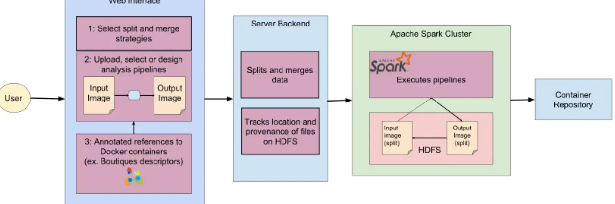
Apache Spark Cluster HDFS Input image (split) Output Image (split) Web Interface Container Repository 3: Annotated references to Docker containers (ex. Boutiques descriptors)

Server Backend Splits and merges

data Tracks location and provenance of files

on HDFS 1: Select split and merge

strategies 2: Upload, select or design

analysis pipelines Input Image Output Image User Executes pipelines

Figure 1: System architecture diagram

That is, the large image will be broken down into splits that are readable by these pipelines such that the image can be processed by the pipelines in parallel. Ideally, our system will be compatible with all frequently used image formats. For now, we will focus on making our system compatible with these three popular image formats: NIfTI-1, NIfTI-2 and MINC 2.0.

As NIfTI-1 is a popular image format in which many neuroimaging pipelines have been de-veloped to be compatible with, we have selected this file format to do our initial development. In addition, unlike MINC 2.0, NIfTI-1 data is stored in a contiguous column-order fashion in a

.niior .img file. This makes a NIfTI-1 image simple to manipulate. As there are only minor differences between NIfTI-1, ANALYZETM7.5, and NIfTI-2, the algorithms and implementations developed should apply to all three of these file types. The algorithms developed should also apply to the MINC 2.0 file format, however algorithm implementation may vary slightly as a result of the file organization difference. To help abstract the main file type differences, we will be using the NiBabel library.

3.4

Partitioning and merging of data

The NIfTI-1 file format is not inherently compatible with distributed environments. To achieve parallelization of a large image and maintain NIfTI readability by NIfTI-aware software, it is

necessary to split the large image into more manageable NIfTI-1 images which can be distributed across the various nodes of the system. Depending on the algorithm used to process the image, it may also be necessary to merge the image back together.

Neuroimaging files may be split into or merged from various schemes such as 2D slices and 3D blocks. As a result of the image size, splitting and merging cannot be achieved in memory. Therefore, splitting and merging must be done chunks at a time. Chunks can represent contiguous data, as in the case of 2D slices or 3D slab, or discontiguous data, as in the case of 3D blocks. In the case of naive splitting and merging (loading one chunk into memory at a time), 2D slices and 3D slabs are expected to be more efficient than 3D blocks. This is due to the fact that seeking must be performed after every discontiguous chunk. As blocks are inherently discontiguous chunks of data, this can lead to frequent seeking which can severely limit performance. Algorithms to reduce seek number will be examined in Chapter4.

During the creation of the splits, an index text file (Figure 2) is generated containing all the HDFS URIs of the splits. These splits will all be stored into the same folder HDFS for later access by the Spark transformations. To merge the splits, the index will be used to locate all the splits and merge them sequentially.

Figure 2: Example of an image index file

3.5

Running pipelines

Pipeline execution will be achieved through the use of Spark transformations and their respective lambda (anonymous) functions. There are two options for loading the splits into Spark and generating an RDD: 1) through reading of the legend file to locate the splits and load them into NiBabel, and 2) providing Spark with the folder name containing all the splits. The first method, using Spark’s functionsc.textFiles()is useful if the splits are not all located in the same folder, however, data locality would not be preserved without some manipulation to the Spark library. This is because YARN will schedule the Spark transformations to execute where the legend file’s chunks

are, which may not necessarily be on the same nodes as the image splits. However, this will only be an issue when the splits are loaded into memory as Spark performs in-memory computations. Nevertheless, split loading may occur more than once in a pipeline. The second option will utilize Spark’s sc.binaryFiles()function to load the images directly from a folder. Data locality is ensured as YARN and Spark are both aware that the RDD needs to be generated from the files in the folder, unlike with the legend. In addition, Spark will load the entire file in memory per compute node, and not just a chunk, which is important as we want to ensure that the image is readable by neuroimaging pipelines. The RDD returned by this method will be in the format of key-value pairs, in which the key is the filename and the value is the image data that can simply be loaded into NiBabel. We will be loading the images into memory using Spark’ssc.binaryFiles()function. As Spark’s transformations implement lazy loading, the entire image will not have to fit in memory to generate an RDD, it is only necessary for splits to fit in memory. Should the pipelines require that the image is saved to disk prior to the execution of another transformation,sc.binaryFiles() can be used again or NiBabel’snib.load()function can be called and data can be extracted prior to ending the transformation and starting the new one such that the new image will be returned as a value.

Executing neuroimaging pipelines can be accomplished through the use of Spark’s map (or other) transformations. The lambda function called by the transformation can call for the execution of a container containing the desired neuroimaging pipelines to execute on the nodes’ data. Should an updated split be saved to disk, NiBabel’s nib.save() function can be called within a Spark transformation.

3.6

Describing pipelines

Users will have the option to use our system’s built-in pipelines or submit their own. Spark pipelines can be encapsulated within a container and referenced to by a descriptor such as Boutiques, or can be provided to our system separately from the container and make calls to functions within transformations that execute the pipelines. For now, we will investigate the latter. To accomplish this, our system requires a URL pointing to a Docker or Singularity container located in a container repository that our cluster can download from. In addition, we will need instructions on how to execute the container.

Chapter 4

Splitting and merging

Note : The following sections of this Chapter contain excerpts from a paper in preparation for IEEE Big Data 2017, in which my contributions were (1) the identification of the blocks vs slices issue, (2) the design of all the algorithms reported in this chapter, (3) the implementation of these algorithms, (4) their extensive benchmarking on two disks.

4.1

Introduction

The process of splitting and merging ultra-high resolution images may significantly impact the performance of our system. However, it also is necessary to split and merge the image in order to parallelize pipeline processing. Therefore, the goal is to find the most efficient algorithms for splitting and merging a large image given for a given split scheme, and to also determine the best performing split schema given the algorithm. Although there are many splitting schemes, we will limit our focus to 3D slabs and 3D blocks.

Intuitively, splitting and merging of slices is expected to be more efficient than blocks as a consequence of the number of seeks required to perform the operation. 3D slabs represent contiguous chunks of data within the NIfTI image, therefore, seek time is limited to file access. In contrast, 3D blocks represent discontiguous chunks of image data, where the number of seeks is a function of the number of file accesses and number of discontiguous chunks. Processing time may also be affected by seek distance. It is known that hard disk drives (HDDs) exhibit variable seek time, whereas solid state drives (SSD) exhibit constant seek time. Therefore, it is hypothesized that the number of seeks will have a subdued effect on seek time in SSDs in comparison to HDDs. To attempt to reduce the seek time incurred by the splitting and merging blocks, we also examined four different merging strategies: (1) naive reading of blocks, (2) naive reading of slabs, (3) clustered

reading of blocks (multiple blocks read and written at once), and (4) buffered reading of slabs (multiple slabs read and written at once). By loading multiple splits into memory at a time, we effectively augment the amount of contiguous data that can be written at a time, thus reducing the overall number of seeks.

Split and merge relate to the same dual problem in our context. We focus here on merging for the sake of concision. Splitting algorithms can be derived from merging ones by swapping reads and writes. Our goal then is to merge a set ofnchunks into a single reconstructed 3D image with Rvoxels of sizeb. For simplicity, we assume that all chunks are of identical size, that they do not overlap, and that slices are squares and blocks are cubes.

4.2

Disk model

A disk is characterized by its read and write rates, its access time and its seek time. For common file sizes, seek time is negligible compared to read or write time as typical seek times range from about 0.1 ms for Solid-State Drives (SSD) to 10 ms for Hard-Disk Drives (HDD). However, as we will shown later, naive algorithms might seek up to 107 times to merge a high-resolution image, which renders total seek time comparable to read and write times. In addition, extensive seeking also has an effect on read and write rates, as these are typically increasing with the duration of uninterrupted reads or writes.

In our analysis, we do not distinguish between access time and seek time. We also assume that seeks require a constant amount of time, regardless of the position seeked to. That is, we focus on the average seek time. In practice, large variations would be expected depending on the seek distance, but modeling such variations would inevitably lead to models specific to the hardware, file system or operating system, which we intentionally avoid here. Likewise, in contemporary systems, read and write times are greatly impacted by caches operating at several levels, which we do not model here. Thus, our goal is to find algorithms that minimize thenumberof seek and file access operations, which we denote “number of seeks” in the remainder.

4.3

Notations

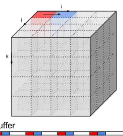
We adopt the following notations (see Figure3):

• R= D3: number of voxels in the reconstructed image. • b: number of bytes per voxel (in B).

• n: number of chunks (blocks or slices).

• m: amount of available memory (in B).

• m: amount of used memory (in B),m ≤ m. We also have the following relations:

• Number of slices, rows, columns in a block: 3 R n = d.

• Number of blocks in a block row: √3

n.

Figure 3: Notations. A block row is shown in red. Ablock slice is shown in blue.

Figure 4: Buffer used in cluster reads (d=4). White portions in the buffer are not allocated.

4.4

Algorithms

4.4.1

Slabs vs blocks

Algorithms 1 and 2 show the naive merging methods for slabs and blocks. These algorithms actually have very different complexities even though blocks and slabs have identical sizes. Since slabs are stored contiguously in the reconstructed image, the number of seeks in Algorithm 1 is only 2nasnseeks are required to read the slabs andnseeks are required to write them:

Nslabs =2n (1)

However, Algorithm2has to do extra seeks for each row in each slice of each block:

or, usingRandnas main variables: Nblocks =n+n 3 r R n !2 (2)

In practice, this difference could lead to a tremendous slowdown, as we will show later.

Algorithm 1Naive merging from slabs foreach slabdo

read slab

write slab in reconstructed image end for

Algorithm 2Naive merging from blocks foreach blockdo

read block

write block in reconstructed image end for

4.4.2

Buffered slabs

Algorithm 1 is a particular case of memory buffering where the amount of available memory equals the maximum size of a chunk. More buffering can be achieved when the amount of available memory increases, as shown in Algorithm 3. This algorithm writes in the reconstructed image

Algorithm 3Buffered merging from slabs

1: sorted_slabs = sort slabs by increasing k values 2: initialize buffer

3: fori = 0 ; i <n ; i+=1 do

4: slice = sorted_slabs[i]

5: ifsizeof(buffer)+sizeof(slab)≥mthen

6: write buffer in reconstructed image 7: clear buffer

8: end if

9: read slab and append it to buffer 10: end for

using a single seek per memory load. Therefore: Nbuff_slab = n+ bR m (3)

Buffered slabs are straightforward to implement, however, their extension to block merging is not easy. The remainder of this Section presents our attempts for such a generalization.

4.4.3

Buffered blocks: Cluster reads

Cluster reads are the more direct extension of buffered slabs to blocks: they load multiple blocks in memory, concatenate them in a buffer and write the buffer in the reconstructed image. Seeking is reduced compared to naive block merging since contiguous parts of the buffer will be written without seeking. A given block is accessed only once.

The buffer might be a slightly complex data structure, for instance an associative array or a Python dictionary, capable of storing multiple disjoint sequences of contiguous bytes without having to allocate memory for the bytes between such sequences. Figure4illustrates how the buffer would fill up for the two first blocks in a reconstructed image, assuming that blocks are of size 4x4x4.

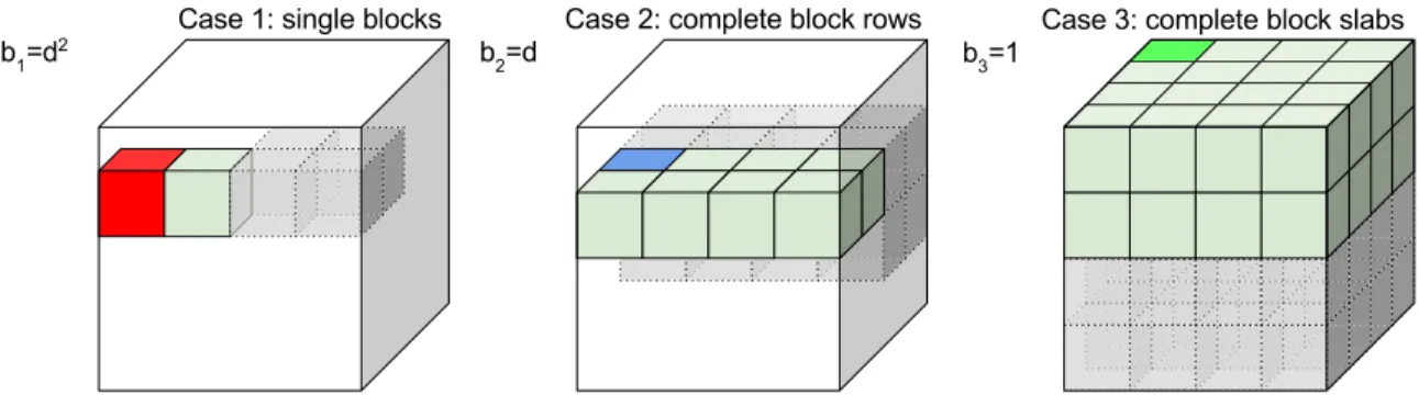
The number of seeks performed by cluster reads depends on how blocks loaded in memory arrange in the reconstructed image. In the best case, complete contiguous slices of the reconstructed image can be assembled in memory and written in a single seek. In the worst case, the memory load only partially covers rows in the reconstructed image: O(d2) seeks are then required during writing, one for every partial row in every partial slice. In the intermediary case, rows are complete but some slices can only be partially reconstructed: O(d) seeks are then required.

Our cluster reads algorithm focuses on the three memory load configurations represented in Figure5, that is, the amount of memorym0used by the algorithm is rounded down to the closest number of complete blocks (case 1), of complete block rows (case 2) or of complete block slabs (case 3). This is in general reasonable since adding an incomplete row to a set of complete ones multiplies the number of required seeks byd, as illustrated in Figure6-Left. In some cases though, rounding m down to m0 might increase the number of required memory loads to a point that the overall number of seeks also increases. Such cases are, however, slightly unusual and their complete description requires extensive calculations involving modulo arithmetic, which we felt were unwieldy to report here.

Our algorithm also avoids configurations where the memory load overlaps multiple block slices in case 2 or multiple block rows in case 1, as such overlaps multiply the number of required seeks (see Figure6-Right).

Figure 5: Memory-load configurations in cluster reads, leading to different number of seeks. Red blocks need seeking before each of their rows (d2 seeks). Blue blocks need seeking before each of their slices (d seeks in total). Green blocks need only a single seek. Grey, dashed, transparent blocks represent the contiguous memory loads and are added for the sake of visualization.

Figure 6: Configurations that increase the number of seeks per memory-load and are thus deliber-ately avoided by cluster reads. Left: configuration with incomplete block rows (multiplies number of seeks byd). Right: configuration with block rows that overlap multiple block slices (multiplies number of seeks by 2).

Cluster reads are described in Algorithm4. Functionswitch (line 3) selects one of the three cases based on the amount of available memory and the number of blocks. It returnsm’andcase, the identifier of the selected case. Function check_overlap (line 7) determines whether two blocks overlap multiple block slices (case 2) or multiple block rows (case 1). For case 3 it always returns false. Functionsizeof(line 8) returns the actual memory used by its argument, including only its allocated segments in the case that the argument is a buffer.

Algorithm 4Buffered merging of blocks with cluster reads 1: sorted_blocks = sort blocks by increasing (k,j,i)

2: initialize buffer

3: (m’,case)=switch(m,n,R,b) 4: old_block = sorted_blocks[0] 5: fori = 0 ; i<n ; i+=1do

6: block = sorted_blocks[i]

7: overlap = check_overlap(block,old_block,case)

8: ifsizeof(buffer)+sizeof(block)≥ m’oroverlap=truethen

9: write buffer in reconstructed image 10: clear buffer

11: overlap = false 12: end if

13: read block and insert it in buffer 14: end for

The amount of memory usedm0is set as follows in each of the 3 cases:

m0₁= Rb n jmn Rb k ;m0₂= Rb 3 √ n2 $ m√3 n2 Rb % ;m0₃= Rb 3 √ n m√3 n Rb

The number of seeks performed by cluster reads in each of the three cases is:

N_CRi =n+ xibi, i ∈n1,3o,

wherexiis the number of memory loads required to reconstruct the image and biis the number of

seeks required to write the memory load. The firstnseeks in the equation are required to read all the blocks at once. According to Figure5, we have:

b1= d2= 3 r R n 2 ; b2= d = 3 r R n ; b3 =1

The numbers of memory loads required to reconstruct the image are: x1= & Rb 3 √ n2m0₁ ' 3 √ n2;x2 = & Rb 3 √ nm0₂ ' 3 √ n;x3= Rb m0₃

Because our algorithm avoids overlapping configurations, x1is proportional to the total number of

block rows in the image (√3_n2_{) and x}

2is proportional to the total number of block slabs ( 3

√

n). Finally, the total number of seeks performed by cluster reads to reconstruct the image is:

NCR=                  n+ Rb 3 √ n2m0 1 3 √ R2 ifm< √₃Rb n2 n+ l Rb 3 √ nm0 2 m 3 √ R if √₃Rb n2 ≤ m < Rb 3 √ n n+ l Rb m₃0 m if Rb√₃ n ≤ m< Rb (4)

It should be noted that NC R is not a continuous function of m, due to the differences among bi

values.

4.5

Implementation

The above algorithms are implemented in Python using Nibabel [25] for image I/O and NumPy for array manipulations.

The data buffer used in Cluster reads is implemented as a Python dictionary where the keys are offsets in the reconstructed image and the values are NumPy arrays containing the data starting at this offset. When the memory load is complete, dictionary entries are written sequentially to the reconstructed image. In naive blocks and cluster reads, some seeking might be required between writes. We implemented a defragmentation procedure for the dictionary that merges contiguous dictionary entries in a single one, but we abandoned it as it proved more time-consuming than going through all the initial entries, due to the overhead of resizing NumPy arrays to merge entries.

4.6

Experiments

4.6.1

Data

We used the 3850x3025x3500 Big Brain image split in 125 non-overlapping chunks of size 770x605x700 with 2 bytes per voxel (total size, uncompressed is 75.92 GB). We used the blocks of the 2015 Big Brain release with 40-micrometer isotropic resolution available atftp://bigbrain. loris.ca/BigBrainRelease.2015/3D_Blocks/40um. We converted them to NIfTI-1 using

3 GB 6 GB 9 GB 12 GB 16 GB

Cluster reads 1 2 2 2 3

Table 1: Algorithm configurations by memory values.

NiBabel and left them uncompressed. We generated NiFTI slabs of size 3850x3025x28 from the reconstructed image, using our naive split algorithm.

4.6.2

Hardware

We used a Dell Precision Tower 3620 workstation with CentOS Linux release 7.3.1611, 32 GB of RAM and two disks. (1) a Hard disk drive (HDD): HGST Travelstar 7K1000, 7200 rpm, 931GiB (1TB), firmware version JB0OA3W0; (2) a Solid-state drive (SSD): SanDisk X400 2.5, 238GiB (256GB), firmware version X4130012. Both drives used 512-byte logical sectors, 4096-byte physical sectors, SATA >3.1 (6.0 Gb/s) and were accessed through the XFS file system v4.5.0. We used iotop(http://guichaz.free.fr/iotop) to monitor I/Os on the workstation and make sure that no other process was compromising our measures.

4.6.3

Execution conditions

Table1shows the configuration of Cluster reads for each memory value, according to Equation4. For instance, Cluster reads are in case 1 for 3 GB. We also did 0 GB of memory for Buffered slices and Cluster reads, which triggered naive slice and block merging. We did 5 repetitions for each memory value. Memory values were shuffled in each repetition, to correct for potential biases coming from ordering, such as caching effects. To improve reproducibility, we dropped the kernel page, dentry and inode caches before each run (echo 3 | sudo tee /proc/sys/vm/drop_caches). We measured the cumulative read, write and seek time in each run, as well as the overhead time defined as the total time minus the sum of all other times.

4.7

Results

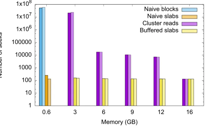
Seeks

The number of seeks is reported in Figure 7, for all algorithms and the corresponding models (Equations1to4). Note the logarithmic y scale. Error bars are not reported as numbers of seeks were constant across all repetitions. The average relative model errors are 12.7% (Naive blocks),

0% (Naive slabs), 3.3% (Clustered reads) and 0.9% (Buffered slabs), explained by the fact that the model assumes cubic blocks while we used non-cubic ones in the experiment. Overall, the model is validated as it correctly explains the observations.

1

10

100

1000

10000

100000

1x10

1x10

1x10

0.6

3

6

9

12

16

Number of seeks

Memory (GB)

Naive blocks

Naive slabs

Cluster reads

Buffered slabs

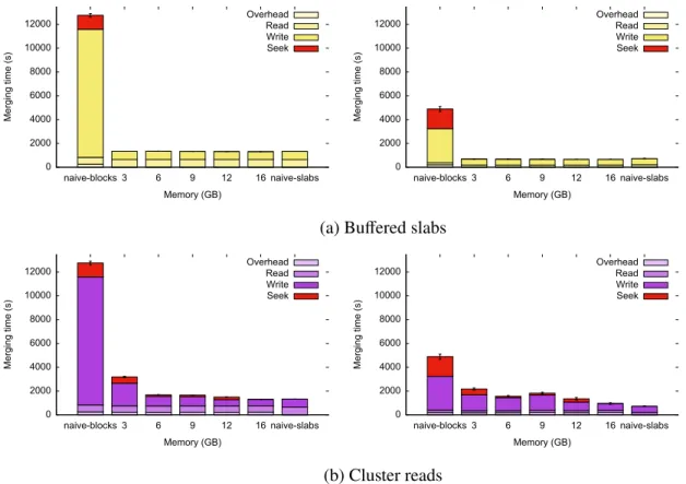
Figure 7: Number of seeks for all algorithms. y scale is logarithmic. Each algorithm is represented with a different color. Dark color is experimental value; bright color is model.

As expected, the difference between naive blocks and naive slabs is tremendous, in the order of 50 million seeks. For 3 GB, the number of seeks in Cluster reads is 5 orders of magnitude higher than naive slices. This huge difference comes from the fact that at 3 GB, Cluster reads are in case 1. For 6 GB, 9 GB and 12 GB, Cluster reads are in case 2 and Buffered slabs reduces. At 16 GB, the algorithms perform the same (Figure8).

Cluster reads provide important speed ups compared to naive blocks, both on HDD and on SSD. On SSD, they are up to 5.1 times faster than naive blocks at 16 GB, and 3.1 on average. On HDD, they are up to 9.7 times faster than naive blocks at 16 GB, and on average 6.8 times faster. Surprisingly, they perform substantially faster than naive blocks even at 3 GB, while in case 1. This may be explained by the fact that the seeks required to write incomplete block rows to the reconstructed image are shorter than the ones for naive blocks.

Merge time breakdown

Figure8show how the total merge time breaks down to read, write, seek and overhead time for our algorithms. Naive blocks and naive slabs are shown as references. The huge difference between naive blocks and naive slabs is coming from both the seek time and the write time, which suggests that seeking degrades the write rate in addition to introducing extra delays. Cluster reads reduce the seek time and thus the read time substantially. The same behaviour is observed on HDD and on SSD, although the effect of seeking is slightly lower on SSD, as expected. Read times are consistently and substantially lower than write times. This may be a result of reading data using Python’s NumPy package, which is more efficient than using native Python - as is the case with our writes. 0 2000 4000 6000 8000 10000 12000 naive-blocks 3 6 9 12 16 naive-slabs Merging time (s) Memory (GB) Overhead Read Write Seek 0 2000 4000 6000 8000 10000 12000 naive-blocks 3 6 9 12 16 naive-slabs Merging time (s) Memory (GB) Overhead Read Write Seek

(a) Buffered slabs

0 2000 4000 6000 8000 10000 12000 naive-blocks 3 6 9 12 16 naive-slabs Merging time (s) Memory (GB) Overhead Read Write Seek 0 2000 4000 6000 8000 10000 12000 naive-blocks 3 6 9 12 16 naive-slabs Merging time (s) Memory (GB) Overhead Read Write Seek (b) Cluster reads

Figure 8: Breakdown of total merge times. Left column: HDD. Right column: SSD.

4.7.1

Conclusion

We have designed and implemented algorithms for the efficient splitting and merging of ultra-high resolution 3D brain images. It is recommended that the image be partitioned into 3D slabs as it offers a significant performance advantage. Should it be necessary to partition the image into

3D blocks, clustered reading of the blocks is suggested as reading several blocks into memory at once will increase performance. If entire block slabs can be read into memory, clustered reads can nearly mimic the performance of buffered slabs. Implementation of the algorithms can be found at https://github.com/big-data-lab-team/sam

As we will process the images on a computing cluster using HDFS, parallel split-and-merge algorithms are required, since the various blocks of a large image would be uploaded to different disks concurrently. In the same vein, “re-spliting” algorithms would have to be devised in case a split image needs to be split in a different geometry. Cluster reads could be used as a starting point for such algorithms.

In terms of file formats, our results demonstrate that simple imaging formats may be split and merged without performance loss compared to more complex formats that try to preserve spatial locality on disk, for instance MINC 2.0 or the format based on space-filling curves mentioned in [26]. This is of major interest in the current open-science context since simpler formats favour data-sharing and interoperability. Moreover, our algorithms could potentially be adapted to any split geometry, even though we demonstrated them on slices and blocks only, while file formats inevitably assume a particular geometry. For instance, the format in [26] is not designed to naively split slices. However, we aimed to extract all the blocks, whereas, [26] aimed to extract a single block from a large image. Furthermore, we have not considered on-the-fly data compression yet, which is a unique feature of MINC 2.0.

Chapter 5

Pipelining framework

5.1

Introduction

Our pipelining framework needs to guarantee efficient execution of neuroimaging pipelines. Lever-aging the features provided by Spark and HDFS in terms of parallelization, data-locality and in-memory computing, we can achieve high performance. Through HDFS, the splits will be di-vided throughout the nodes and replicated in case of node failure. YARN will schedule Spark computations to occur closest to the data node to preserve data locality. Spark will load the data lo-cated at that node to the node’s memory to eliminate input andoutput (I/O) time that would occur as a consequence of reading to and from disk at every map and reduce phase for every transformation. In this Chapter we describe and benchmark the first use of Apache Spark for high-resolution 3D neuroimaging. The various use cases will examine the effects of parallelization of a neuroimaging pipeline with and without a Docker container, as well as the effect that in-memory computing has on total processing time.

5.1.1

Describing neuroimaging pipelines in Spark

For neuroimaging pipelines to process the splits in parallel, they will be executed on the split image data within a Spark transformation. In order to generate an RDD of NIfTI images, the directory containing the images is read using Spark’ssc.binaryFiles. The RDD created from reading the directory is a collection of key-value pairs, where the key represents the image filename, and the value is the binary representation of the image. Once the RDD of NIfTI images is generated, image data can be manipulated directly within lambda functions with the help of NiBabel. As containers have no ability to access the node’s in-memory data directly, a directory containing the splits will have to be mounted onto the container. This can be accomplished by writing RDD data in a lambda

function to the local filesystem or by writing to a volatile temporary filesystem, if available, such as Linux’s tmpfs. The container will then be able to process the pipeline and save results to the mounted directory, which can then be loaded back into Spark using NiBabel, for further processing.

5.1.2

Hardware

All tests were performed on Amazon EC2 m4.16xlarge Centos 7 instance with 64 virtual Intel(R) Xeon(R) CPUs E5-2686 v4 @ 2.30GHz and 256GB RAM.

5.1.3

Data

As with the previous chapter, the image selected to perform such tests was the 40µm resolution BigBrain image. The BigBrain was split prior to these tests into 770x605x700 non-overlapping compressed NIfTI blocks.

5.2

Effects of parallelization on neuroimaging pipelines

5.2.1

Histogram computation

As a first use case, we analyzed the effects of parallelization on a simple histogram computation. For this, we looked at how varying the number of pipeline executors would affect processing time. Algorithm5shows how the pipeline was implemented. Once images were loading into a Spark RDD as described in 5.1.1, the image data was separated from the header contents to generate a histogram. This was achieved by reading the binary data stored in the RDD into NiBabel and extracting data using NiBabel’s img.get_data function inside the lambda function of a Spark flatMap transformation – a transformation which allows each input item to be mapped to 0 or more output items. The lambda function returned the filename as key, and a NumPy array of image data as value. To generate the histogram, it is necessary to obtain the minimum and maximum voxel value of the image. To achieve this, a flatMap transformation is used and the lambda function called by the transform will return the minimum and maximum for each respective image. These results are then collected onto one node, and the min and max of the image is obtained by sequentially iterating through the list of split minima and maxima. AflatMaptransformation can then be applied again on the RDD containing the image data to generate an RDD containing the 5-bin histogram of the splits with given minimum and maximum. To finalize the generation of the histogram, a reduceByKey transform is called on the recently generated RDD to collect all

split histogram frequencies belonging to the same bin into the same compute node to sum their frequencies together. The RDD data was then collected into one node and printed to screen.

Algorithm 5Spark pipeline for histogram computation 1: min, max = None

2: binRDD = load directory of binary files in Spark 3: nibRDD = binRDD.map(load image array)

4: minmax = nibRDD.flatMap(get min and max).collect() 5: forelement in minmaxdo

6: ifelement less than minthen

7: min = element 8: end if

9: ifelement greater than maxthen

10: max = element 11: end if

12: end for

13: histogram = nibRDD.flatMap(create histogram).reduceByKey().collect()

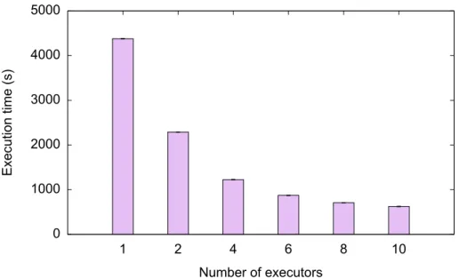
0 1000 2000 3000 4000 5000 1 2 4 6 8 10 Execution time (s) Number of executors

Figure 9: Average histogram computation times over 1, 2, 4, 6, 8 and 10 executors. 5 repetitions were performed for each executor amount.

We benchmarked our implementation using 1, 2, 4, 6, 8 and 10 executors, respectively. The number of cores per executor was 1, and the amount of memory allocated to an executor instance

was 10 GB. For all executions, the histogram returned contained 5 bins.

The resulting data, as seen in Figure 9 suggests that the neuroimaging pipelines, such as the above, scales well to an increased number of executors. The algorithm runs almost 7 times faster with 10 executors than with only one. However, there is a limit to the amount of speedup that can be provided by executing pipelines in parallel. This can be observed through the speedup reduction as the number of executors decrease. Such behaviour can be explained by the non-parallelizable steps, such ascollectactions, which limit the amount of parallelization.

5.2.2

Containerized pipeline

The neuroimaging pipelines used to process the images need to be containerized. As a second use case, we examined the effects of parallelization on a containerized pipeline. A script making a call to the FSL binarization command was built into a Docker container.

The Spark algorithm (Algorithm 6) was similar to that of the histogram algorithm above, however the minimum and maximum did not need to be obtained and the data was not reduced at the end as we wanted to return the binarized splits.

Algorithm 6Map transformation’s lambda function for containerized pipeline execution 1: Input:(filename, binary image, output folder, threshold)

2: Output:(filename, binarized_image)

3: image = load binarized binary image into NiBabel 4: nibabel.save(image, current working directory) 5: mount directory into container and execute pipeline 6: binarized_image = read image from disk

To share the image splits within the container, the RDD data of each node was written to the node’s respective home directory. This directory was then mounted in the container in order for the pipeline to binarize the splits within the container. The updated images were then saved onto the shared directory, and uploaded onto HDFS for potential future processing by other pipelines.

Figure 10 show that parallelization of containerized pipelines scales just as well as non-containerized pipelines in spite of the overhead of using containers. These results suggest that parallelization will significantly reduce processing of containerized pipelines. Since speedup ta-pers down as parallelization increases due to non-parallelizable steps limiting speedup and the fact that many neuroimaging pipeline steps will likely not be parallelizable, and speedup will be limited. Nevertheless, the initial speedup from partitioning the large image into smaller constituents and processing those in parallel is still expected to be significant.