Ultrafast ultrasound imaging as an inverse problem:
Matrix-free sparse image reconstruction
Adrien Besson,
Student member,
Dimitris Perdios,
Student member,
Florian Martinez, Zhouye Chen,
Student
member,
Rafael E. Carrillo,
Member,
Marcel Arditi,
Senior member,
Yves Wiaux, Jean-Philippe Thiran,
Senior
member
Abstract—Conventional ultrasound (US) image reconstruction methods rely on delay-and-sum (DAS) beamforming, which is a relatively poor solution of the image reconstruction problem. An alternative to DAS consists in using iterative techniques which require both an accurate measurement model and a strong prior on the image under scrutiny. Towards this goal, much effort has been deployed in formulating models for US imaging which usually require a large amount of memory to store the matrix coefficients. We present two different techniques which take advantage of fast and matrix-free formulations derived for the measurement model and its adjoint, and rely on sparsity of US images in well-chosen models. Sparse regularization is used for enhanced image reconstruction. Compressed beamforming exploits the compressed sensing framework to restore high quality images from fewer raw-data than state-of-the-art approaches. Using simulated data and in vivoexperimental acquisitions, we show that the proposed approach is three orders of magnitude faster than non-DAS state-of-the-art methods, with comparable or better image quality.
Index Terms—Ultrafast ultrasound imaging, compressed sens-ing, beamformsens-ing, sparse regularization
I. INTRODUCTION
Ultrasound (US) imaging is one of the most used medi-cal imaging modalities enabling real-time, safe and low-cost procedures such as fetal, abdominal and cardiac imaging. Recently, a new paradigm, denoted as ultrafast US imaging, has enabled US imaging to reach more than thousands of frames per second, paving the way to a whole range of new applications such as tracking of induced and intrinsic shear waves in organs [1].
Pulse-echo US imaging uses an array of transducer elements to transmit short acoustical pulses through the body. The backscattered echo waveforms are then received by the same array and detected as so-called element raw-data. Retrieving an image of the medium inhomogeneities from the element raw-data poses an ill-posed inverse problem. Current real-time US imaging is generally based on the well-known delay-and-sum (DAS) beamforming algorithm which can be seen as a back-projection solution of the inverse problem under several A. Besson, D. Perdios, F. Martinez, M. Arditi and J.-Ph. Thiran are with the Signal Processing Laboratory 5 (LTS5), Ecole Polytechnique F´ed´erale de Lausanne, CH-1015, Lausanne, Switzerland.
R. E. Carrillo is with the Centre Suisse d’´electronique et microtech-nique (CSEM), CH-2002 Neuchˆatel, Switzerland.
Z. Chen and Y. Wiaux are with the Institute of Sensors, Signals and Systems, Heriot-Watt University, EH14 4AS Edinburgh, United-Kingdom.
J.-Ph. Thiran is also with the Department of Radiology, University Hospital Center (CHUV) and University of Lausanne (UNIL), CH-1011, Lausanne, Switzerland.
assumptions [2]. While being suitable for real-time imaging, DAS suffers from a relatively low quality, in terms of signal-to-noise ratio, and requires sampling the element raw-data at a rate few times higher than the Nyquist rate for sufficient accuracy in the delay calculations [3], [4].
An alternative to back-projection methods consists of sparse regularization (SR) techniques [5]. These methods are built upon forward models of the problem and introduce additional information on the signal under scrutiny in order to solve the ill-posed inverse problem, leading to a higher image quality than back-projection methods.
Medical imaging is well-suited to SR methods. Indeed, in many medical imaging modalities, the image reconstruction process amounts to solving a linear inverse problem. In magnetic resonance imaging (MRI), the image is reconstructed from k-space samples and the measurement model is an inverse Fourier transform [6]. In X-ray computed tomogra-phy (CT), the sinogram is related to the measurements by the Beer-Lambert law which can be expressed as a linear inverse problem in the discrete domain [7]. Moreover, sparsity priors have been expressed for medical images. Lustiget al.[6] have exploited sparsity of MRI images in the wavelet domain and under the total-variation (TV) transform. In X-ray CT, sparsity priors under the TV-norm have been extensively used [8], [9]. In US imaging, several formulations of forward models have been recently investigated. David et al. [10], Wang et al. [11] and Besson et al. [12] have proposed time-domain formulations of the problem. In the Fourier domain, Zhanget al.[13] have suggested a formulation of the model derived by Davidet al.[10]. Bessonet al.[14] have presented a forward model in the Fourier domain in which US propagation is seen as a projection on a non-uniform Fourier space. Schiffner and Schmitz [15] have proposed a time-frequency model in which each frequency of the transducer-element bandwidth is treated independently, enabling the model to deal with distortion effects. The main problem of these models resides in their computational complexity, usually translated in storage requirements of the corresponding matrix representation. The models proposed by David et al. [10] and Schiffner and Schmitz [15] require the storage of several hundreds of GB for matrix coefficients in 2D. Zhang et al.[13] have divided the image in stripes in order to make the problem tractable. This issue severely limits the appeal of iterative methods against classical approaches. Ozmenet al.[2] have suggested the use of matrix-free operators but did not provide any implementation detail and only applied their model to low
frequencies.
SR methods have raised a growing interest recently in US imaging. They have been used for despeckling [16], [17] and deconvolution [18], [19] of radio-frequency images. They have been exploited to solve inverse scattering problems,e.g.using the constrast-source-inversion method [2]. They have also been used in the context of the compressed sensing (CS) framework. It has been explored in a pre-beamforming step, where the problem has been formulated on the element raw-data [20]. It has also been investigated in a post-beamforming step in order to reduce the amount of data to be stored [21], [22] as well as combined with a deconvolution framework for image enhancement [19]. In a similar direction, it has been used in the image reconstruction process, in order to reduce the amount of data necessary to retrieve a high quality image either by reducing the number of transducer elements [10], [12] or by sub-Nyquist rate sampling [4], and to improve the image quality compared to backprojection methods [13], [14], [15], [23], [24], [25], [26].
Three main contributions are proposed in this work. Firstly, parametric, fast and matrix-free formulations of the measure-ment model and its adjoint are described for both plane-wave (PW) and diverging-plane-wave (DW) compounding. Secondly, a fully parallel implementation of these formulations is in-cluded in a sparse regularization framework, resulting in high-quality imaging with near real-time capability and no memory footprint, paving the way to sparse regularization for 3D US imaging. Lastly, the proposed model is coupled with innovative compression strategies which outperform existing compressed beamforming (CB) schemes [10], [12].
The remainder of the paper is organized as follows. The matrix-free formulations of the measurement model and its adjoint are described in Section II. The proposed image reconstruction method is described in Section III and evaluated on simulated and in vivo data in Section IV. Results are reported in Sections V and VI and discussed in Section VII. Concluding remarks are given in Section VIII.
II. PARAMETRIC MATRIX-FREE FORMULATIONS OF THE MEASUREMENT MODEL AND ITS ADJOINT
A. Formulation of the measurement model
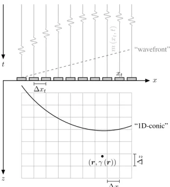
Ultrafast US imaging involves transmission of either steered PW (SPW) or DWs. In this case, it has been shown that one may express the image reconstruction as an inverse problem [10], [15]. More precisely, let us consider a pulse-echo experiment, described on Figure 1, where the propagation medium Ω∈R2\ {z≤0} contains inhomogeneities as local
fluctuations in acoustic velocity and/or density, defining a tissue reflectivity function (TRF) γ(r) with r = [x, z]T ∈
Ω [15], [27]. The medium is insonified with a 1D-array of
Nel transducer elements, located atrt= [xt,0] T
, wherext∈ Ξ⊂R, and the echo signals detected by the same elements are
m ( xt , t ) (r, γ(r)) xt x z t “wavefront” “1D-conic” ∆x ∆ z ∆xt
Fig. 1: Standard 2D-ultrafast ultrasound imaging configura-tion.
denoted asm(xt, t). Thus, the following relationship holds:
m(xt, t) =
Z
r∈Ω
od(r, xt)γ(r)
vpe(t−tT x(r)−tRx(r, xt))dr, (1)
which can be rewritten as:
m(xt, t) = Z Z τ∈R,r∈Γ(xt,τ) od(r, xt)γ(r) | ∇rg| dσ(r)vpe(t−τ)dτ, (2) wherevpe(t) denotes the pulse-echo waveform, od(r, xt) is
defined as od(r, xt) =o(r, xt)/(2π q (x−xt) 2 +z2), (3)
witho(r, xt)the element directivity according to Selfridgeet
al. [28],g(r, xt, t)is defined as:
g(r, xt, t) =t−tT x(r)−tRx(r, xt), (4)
withtT x(r)the propagation delay in transmit andtRx(r, xt)
the propagation delay in receive defined as:
tRx(r, xt) =
q
(x−xt) 2
+z2/c, (5)
∇rg denotes the gradient of g with respect to the variabler
anddσ(r)is the measure over the 1D-curveΓ (xt, t)defined
as:
Γ (xt, t) ={r∈Ω|g(r, xt, t) = 0} (6)
This model is a pulse-echo-spatial-impulse-response model firstly introduced by Tupholme [29] and Stepanishen [30], later used by Jensen and Svendsen [31].
Equation (2) can be written as follows: m(xt, t) = Z τ∈R h(xt, τ)vpe(t−τ)dτ, (7) where h(xt, t) = Z r∈Γ(xt,t) od(r, xt)γ(r) | ∇rg| dσ(r). (8)
Let us now introduce the parametrization z = z(x, xt, t) of
the 1D-conic described by Γ (xt, t). The curvilinear integral
defined in Equation (8) can then be recast as the following 1D integral: h(xt, t) = Z x∈R od(x, z(x, xt, t), xt) | ∇(x,z(x,xt,t))g| γ(x, z(x, xt, t))|Jz(x)|dx, (9) where|Jz(x)|= q 1 + dxdz2
is the Jacobian associated with the parameterization of the curve.
The parametric formulations used in Equation (8) depend on the transmit scheme and are expressed in Appendix A for PW and DW imaging, respectively.
Let us introduce the lateral position of the j-th transducer element, given byxjt =x0
t+j∆xtwith∆xtthe pitch andx0t
the position of the reference transducer element. Let us also consider that the pulse-echo experiment is achieved at time samples tl=t0+l∆t, for l∈ {1, ..., N
t}, where ∆t= 1/fs,
fsis the sampling frequency andt0 the initial recording time
sample. Let us also introduce the image grid defined by xn=
x0+n∆x andzq =z0+q∆z with(n, q) ∈ {1, ..., Nx} ×
{1, ..., Nz}.
It is demonstrated, in Appendix B, that, for each samples of the element-raw data, the following relationship holds:
mxjt, tl=Hγ, xjt, tl+ν0xjt, tl, (10)
whereγ∈RNx×Nz are the values of the TRF evaluated on the image grid defined above, His the matrix-free measurement model and ν0xjt, tl
is the noise which accounts for the model, interpolation and measurement errors.
The signal received by the j-th transducer element can thus be written as a vector mj ∈ RNt which contains
the backscattered echoes from the medium, recorded at time samples defined above. By concatenating the signals sensed by all the transducer elements in a single vector, one may come up with a measurement vector m∈RNelNt.
B. The adjoint of the proposed measurement model and its relationship with the delay-and-sum algorithm
Image reconstruction methods, either analytical or iterative, require the computation of the adjoint of the operator defined in Equation (10) [5]. Indeed, back-projection methods are based on applying the adjoint operator of the measurement model. In regularization approaches, the adjoint operator is used at each iteration of the reconstruction algorithms.
In this section, we derive the adjoint of the measurement model proposed in Section II-A. First, it is demonstrated that
the adjoint operator of the continuous forward model described in Equation (2) can be written as:
ˆ γ(r) = Z xt∈Ξ od(r, xt) (m(xt)∗tu) (tT x(r) +tRx(r, xt))dxt, (11)
whereu(t) =vpe(−t)is the matched filter corresponding to
vpe. The proof of Equation (11) is given in Appendix C.
Thus the parameterization of the adjoint operator is straight-forward sincet=tT x(r) +tRx(r, xt). A matrix-free
formu-lation of the adjoint operator can therefore be derived, for each point of the image grid, which leads to the following relationship:
ˆ
γ(xn, zq) =H?(m, xn, zq) +ξ0(xn, zq), (12)
where H? is the adjoint operator described in Appendix B
and ξ0(xn, zq) is the noise which accounts for the model,
interpolation and measurement errors.
The DAS algorithm is the standard image reconstruction method employed in US imaging because of its simplicity and real-time capability. The DAS algorithm can be mathe-matically formulated as:
γDAS(r) =
Z
xt∈Ξ
a(r, xt)m(xt, tT x(r) +tRx(r, xt))dxt,
(13) where a(r, xt) accounts for the apodization weights, and
γDAS(r) is the DAS estimate of the TRF. In the light of Equation (11), it is demonstrated that DAS achieves a back-projection solution of the inverse problem when the effect of the pulse-echo waveform is neglected (uconsidered as a Dirac) and when the apodization weightsa(r, xt)are set to be equal
tood(r, xt).
Such solution can therefore be straightforwardly defined in the context of the adjoint operatorH?:
γDAS(xn, zq) =HDAS(m, xn, zq) +ξDAS(xn, zq), (14)
where HDAS denotes the approximation of the operator H?
and ξDAS(xn, zq) is the corresponding noise, taking into
account the assumptions of DAS.
The DAS solution, while suited to real-time imaging, is therefore a relatively poor approximation of the solution of Problem (2). Indeed, DAS beamforming does not address the problem of the noise n, neglects pulse-shape, and requires a sampling rate higher than Nyquist sampling requirements because of the high-delay resolution required [3], [4]. Indeed, to apply the delay defined in Equation (13) digitally, received signals must be sampled on a sufficiently dense grid.
C. The inverse problem of interest
In the literature, two different groups of image reconstruc-tion methods may be distinguished, since they aim at solving two different problems.
The first group of methods can be denoted as regularized beamforming methods. They do not take into account the pulse-echo waveform and retrieve a low-resolution estimate
of the TRF γ, usually denoted as the radio-frequency (RF) image γRF [11], [12], [23], [24], [32], [33]. One reason for
this choice resides in the fact that γRF preserves speckle
information (due to the low-resolution), which is of interest in many US applications.
The second group of methods aims at performing inverse scattering, i.e. at retrieving the high-resolution TRF γ from the element-raw data [2], [10], [15]. This problem is far more complex, highly ill-posed, and usually requires more sophisti-cated models than the ones used for regularized beamforming methods.
While the model described in Section II can be used for inverse scattering problems, we focus, in this work, on regularized beamforming, which means that we neglect the effect of the pulse-echo waveform vpe in the model. This
results in approximating the pulse-echo waveform as a Dirac delta function and Equation (2) is greatly simplified as:
m(xt, t) = Z r∈Γ(xt,t) od(r, xt)γ(r) | ∇rg| dσ(r). (15)
Moreover, it can be noticed that Equation (10) can be ex-pressed using a matrix formalism, leading to a more standard formulation of the inverse problem as:
m=HRFγRF+νRF, (16)
where HRF ∈ RNelNt×NxNz and νRF ∈
RNelNt are the operator and the noise evaluated at each sample of the element-raw data grid.
In the light of Problem (16), the DAS estimate described in Section II-B can be seen as a low-quality estimate of γRF.
III. SPARSITY-DRIVEN IMAGE RECONSTRUCTION METHODS
A. A quick tour on sparse regularization and compressed sensing
1) Sparse regularization: Regularization techniques
intro-duce additional prior information to solve an ill-posed linear inverse problem of the form y = Φs+n, where y ∈ CM
are the measurements, s ∈CN is the image under scrutiny, Φ ∈ CM×N is the measurement model and n ∈ CM is the
observation noise. The problem associated with regularization techniques is of the following form:
min
s F(Φs,y) +βR(s), (17)
whereFis a distance function betweenΦsandy,Ris a non-negative functional, which accounts for the prior information on s, and β denotes the regularization parameter. One well-known technique is Tikhonov regularization in whichRis the
`2-norm. It has been studied by Szasz et al. [33] in the case
of US image reconstruction.
SR techniques offer an alternative to Tikhonov regulariza-tion and exploit a sparsity prior of the signals of interest under a given model Ψ, usually expressed in terms of the`1-norm.
The following problem is thus expressed:
min s kΦs−yk 2 2+λkΨ †sk 1, (18)
whereΨ† accounts for the adjoint operator ofΨandλis the regularization parameter. Problem (18) can also be written as:
min
s kΨ
†sk
1 subject toky−Φsk2≤, (19)
where is a upper bound of the `2-norm of the noise.
Prob-lems (18) and (19) can be solved using convex-optimization al-gorithms such as primal-dual-forward-backward (PDFB) [34], used in the proposed work and described in Appendix D.
2) Compressed sensing: The now famous theory of CS
introduces a signal acquisition framework that goes beyond the traditional Nyquist sampling paradigm [35], [36], [37]. CS demonstrates that sparse or compressible signals can be acquired using a small number of linear measurements and recovered by solving a non-linear optimization problem [35], [36], [37].
Formally, the signal sis acquired through the linear mea-surement model Φ∈CM×N and y=Φs+nas defined in
Section III-A1. WhenM < N, recoveringsfrom yamounts to solving an ill-posed inverse problem and CS demonstrates thatscan be recovered exactly fromy, with high probability, by solving Problem (19).
If we consider a matrix A = [a1, ...,aL] ∈ CM×L, its
mutual coherence is measured as:
µ(A) = max k,j,k6=j
|<ak,aj >|
kakk2·kajk2
, (20)
where<·,·>accounts for the inner-product inCM.
Theorem 3.1 from [35] tells us that the perfect recovery condition ofs relies on a trade-off between the coherence of
A and the sparsity of Ψ†s. It can be shown that µ(A) lies between the Welch bound [38] and 1. The Welch bound gives a higher bound on the sparsity of the solution [35]. Putting everything together, to maximize the benefits of Theorem 3.1 from [35], one should be able to:
• build a measurement modelΦin such a way thatµ(ΦΨ)
is as close as possible to the Welch bound;
• build a sparsity modelΨin such a way thatα=Ψ†sis
as sparse as possible.
B. Sparse regularization for enhanced ultrasound image re-construction
SR for enhanced US image reconstruction proposes an alter-native to DAS for solving Problem (16) by exploiting the SR framework described in Section III-A1. Indeed, Problem (16) is an ill-posed linear inverse problem, thus suited to the SR framework. The underlying idea consists of the introduction of a sparsity prior on RF images in a well-chosen model, described hereafter, in order to recover a high quality image by solving Problem (19).
The sparsifying model Ψ, denoted as sparsity averag-ing (SA) is composed of a concatenation of 8 Daubechies wavelet transforms with different mother wavelets ranging from Daubechies 1 (db1) to Daubechies 8 (db8) [39]. The operator is written as:
Ψ=√1
where q is equal to 8 and Ψi denotes the i-th Daubechies
wavelet transform. The choice of the SA model is justified by its superior results on US images [14], compared to simpler wavelet-based models.
C. Compressed beamforming
CB aims at reducing the amount of data needed to recover high-quality US images. It is built upon the CS framework described in Section III-A2.
To account for the undersampling process, supposed to be linear, we introduce a matrix D ∈ RM×NelNt, with M ≤
NelNt, such that md =Dm and Hd =DHRF. The inverse
problem can be naturally expressed as:
md=HdγRF+νd, (22)
whereνd∈RM accounts for the noise.
CB uses SR approaches, described in Section III-A, to solve Problem (22). The sparsity prior is expressed in the SA model and CB exploits the requirements of Theorem 3.1 from [35] for the design of the undersampling operator D.
The perfect recovery condition of CB relies on the incoher-ence between the measurement modelHd and the sparsifying
model Ψ. In the case of US imaging, the measurement model
His imposed by the problem and the undersampling operator
Dshould be defined in such a way that the coherence between
Hd andΨis minimized.
1) Selection of transducer elements: In our previous work
[12], we have proposed several designs for the undersampling operator which selects a subset of transducer elements, either uniformly- or randomly-spaced. In this case, the operator
D selects the transducer elements of interest. It has been shown that high quality reconstructions may be achieved with approximately 40 % to 50 % of the initial data, for PW and DW imaging [32]. However, the corresponding measurement model Hd suffers from a high coherence [10], [12].
2) Mixing of the raw data: Taking into account the increase
of the coherence induced by these simple undersampling schemes, one may think about designing a strategy such that the mutual coherence of the measurement operator is optimized. The underlying idea is to spread the information as much as possible between the element raw-data space and the desired-image space, hence lowering the coherence, similarly to sparse MRI acquisition [6]. Put formally, we introduce a linear operator W∈RNelNt×NelNt such that D=PW, where P∈RM×NelNt represents an undersampling operator.
The relationship between the desired-image space and the element raw-data space is described by projections onto 1D-conics. It can be deduced that only few samples of the desired-image space are contributing to every samples of the element raw-data space, leading to a highly coherent measurement model.
Nevertheless, it is interesting to note that each point of the element raw-data space generates a different conic in the desired-image space. Since two non-identical conics may intersect on four points at most, the information contained in different samples of the element raw-data space are comple-mentary. Taking into account such an observation, our idea
consists in mixing the information contained in various points of the element raw-data space in order to increase the amount of information carried by each measurement, which may lead to a lower coherence of the matrix.
Formally, the matrix W is designed as a random matrix,
i.e. with i.i.d. entries drawn from a probability distribution.
If we denote by mxjt, tl
the element raw-data received at sample tl by the transducer element positioned at xjt and by
mW xkt, tu
the mixed element raw-data samples at sample
tu on the synthetic mixed channelxk
t, the following equation
holds: mW xkt, t u = Nel X j=1 Nt X l=1 wjlkum xjt, tl, ∀k∈ {1, ..., Nel}. (23) wherewjlku are drawn from a probability distribution. It can
be observed that each mixed element raw-data mW xkt, tu
is related toγRF(xn, zq)by an integration onΓ W xkt, tu = Nt S l=1 Nel S j=1 Γxjt, tl, where Γxj t, tl is a 1D-conic defined in Section II-A. Since each 1D-conic carries complementary information about the desired-image space, it can be stated that Γxjt, tl
⊂ΓW xkt, tu
.
Finally, one can vectorize Equation (23) in order to come up with the following equation:
md=PWm, (24)
The main drawback of this strategy resides in the design of the linear operator W. As an example, if we consider element raw-data acquired over 1000 depth samples, with 128 transducer elements, and that the grid of the desired image is the same as the grid of the element raw-data, thenWrequires 131 GB of memory to store the matrix coefficients, in double precision. In order to overcome this drawback, two strategies, denoted as ‘Channel mixing’ (CMIX) and ‘Channel and time mixing’ (CTMIX) are proposed.
CMIX consists of a random summation of the signals coming from the different transducers elements at a given time instant in order to create a mixed output. In this case, Equation (23) becomes: mW xkt, t u = Nel X j=1 wjkum xjt, tu, ∀k∈ {1, ..., Nel}. (25) The matrixWonly containsNel values per row which
drasti-cally reduces its complexity. In addition, such a mixing could be achievable in hardware, providing a probe which integrates a system able to perform CMIX in a pre-beamforming step. However, it is clear that the mixing and resulting coherence reduction effects of CMIX are rather limited compared to a fully random mixing.
CTMIX extends the principle of CMIX by considering mixing across both transducer elements andDt time samples
to limit the complexity. Put formally, the following relationship holds: mW xkt, t u = Nel X j=1 Dt X l=1 wjlkum xjt, tl, ∀k∈ {1, ..., Nel}, (26) in which the samples tl are chosen randomly in the entire range of time. When Dt = Nt, CTMIX is equivalent to the
case where a fully random matrix is used. When Dt=1 and
tl=tu, CTMIX is equivalent to CMIX.
IV. EXPERIMENTS
A. Experimental setup
1) Plane wave imaging: All the measurements (except the
ones from the PICMUS dataset) are achieved with a standard linear-probe (designed to work at 7.8 MHz) whose settings are given in Table I. For each experiment, a sequence of 15 SPWs (5 MHz, 1-cycle, tri-state waveforms) is transmitted with steering angles uniformly distributed between −7.5◦ and 7.5◦. No apodization is used on transmit.
TABLE I: Characteristics of the ATL L12-5 50 mm probe used for PW imaging. Parameter Value Number of elements 128 Center frequency 5 MHz Wavelength 0.31 mm Sampling frequency 31.2 MHz Pitch 0.195 mm Kerf 0.05 mm
• Numerical simulations: The system described above is simulated using Field II software [31]. Two phantoms are insonified:
– Point-reflector phantom: It consists of bright
reflec-tors laterally positioned at 5 mm and spaced in depth by 10 mm. At depths of 10 mm and 30 mm, bright reflectors are distributed laterally with a step of 5 mm.
– Anechoic-inclusion phantom: It consists of an
ane-choic inclusion of 8 mm diameter, centered at a depth of 40 mm, embedded in a medium with a high density of scatterers with random positions and amplitudes (20 scatterers per resolution cell).
• PICMUS dataset:The methods are also evaluated on the
standardized PICMUS dataset [40]. More precisely, the simulated dataset as well as thein vivocarotids are used. The corresponding settings are available on the PICMUS website1.
• In vivo experiments: Two in vivo carotid images were acquired using a Verasonics US scanner (Redmond, WA, USA) with the ATL probe whose settings are given in Table I.
1https://www.creatis.insa-lyon.fr/Challenge/IEEE IUS 2016/home
2) Diverging wave imaging: All the measurements are
performed with a simulated phased-array probe whose settings are given in Table II. For each experiment, a sequence of 15 DWs (2.5 MHz, 1-cycle, tri-state waveforms) is transmitted with virtual point sources located atzn equal to −2.9 mm and
uniformly distributed atxnbetween −5.9 mm and 5.9 mm. No
apodization is used on transmit.
TABLE II: Characteristics of the probe used for DW imaging.
Parameter Value Number of elements 64 Center frequency 2.5 MHz Wavelength 0.62 mm Sampling frequency 15.6 MHz Pitch 0.32 mm Kerf 0.05 mm
• Numerical simulations:We exploit the numerical simu-lation of the following phantoms:
– Point-reflector phantom: It consists of bright
re-flectors centered in the field and spaced in depth every 20 mm. At 50 mm depth, bright reflectors are laterally distributed with a step of 20 mm.
– Anechoic-inclusion phantom:The anechoic-inclusion
phantom is the same as for the PW experiment.
B. Image recontruction methods
The proposed image reconstruction methods are evaluated against classical DAS algorithm as well as against best state-of-the-art image reconstruction algorithms on the PICMUS dataset, based on the log-compressed B-mode image. The envelope image is extracted from the US RF-image through the Hilbert transform, log-compressed over a range of 40 dB and finally converted to 8-bit gray scale to get the B-mode image.
The DAS algorithm used in this study is the one described by Montaldoet al. [41] for PW imaging and by Papadacciet al.[42] for DW imaging. It is used with a linear interpolation for delay calculations and with a factor correcting for the obliquity. For the iterative approaches, the measurement model and the adjoint described in Section II are used with a linear interpolation. The hyper-parameters of the optimization algo-rithm are empirically tuned depending on the reconstruction method. The stopping criterion is set to be a maximum number of iterations.
C. Computation time
The proposed image reconstruction methods are imple-mented on a NVIDIA Titan X GPU card for evaluation in terms of computation time. The timings are calculated as an average computation time over 500 draws of each reconstruction method. It has to be noted that the proposed implementation is not optimized and a substantial gain may be achieved by working on simple acceleration strategies.
V. RESULTS: SPARSE REGULARIZATION FOR ENHANCED IMAGE RECONSTRUCTION
As explained in Section III-B, SR is a powerful framework to solve ill-posed inverse problems. In this section, we expose
the results obtained with SR on the simulated point-reflector and anechoic-inclusion phantoms (described in Section IV-A), for both PW and DW imaging. We also present results on the
in vivocarotid images obtained with PW imaging. We finally
compare SR to the best state-of-the-art mage reconstruction algorithms on the PICMUS dataset.
A. Contrast study on the anechoic-inclusion phantom
In order to evaluate image contrast, the anechoic-inclusion phantom is used. The proposed method is coupled with a sparsity prior in the SA model described in Section III-B. The maximum number of iterations is set to 50. The dB contrast-to-noise ratio (CNR) [43] is calculated on the normalized envelope image, i.e. on the envelope image divided by its maximum value, using the following formula:
CNR= 20 log10|qµt−µb| σ2
t+σ2b
2
, (27)
where (µt, µb) and (σt2, σb2) are the means and the variances
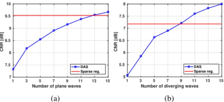
of the target inclusion and the background, respectively. Figures 2a and 2b display the CNR values for PW and DW imaging, respectively, with 1 insonification for the proposed approach and 1 to 15 insonifications for DAS. It can be noticed that, with only 1 insonification, the proposed method leads to a contrast similar to DAS with more than 9 insonifications, and considerably better than DAS for 1 to 9 insonifications.
1 3 5 7 9 11 13 15
Number of plane waves 7 7.5 8 8.5 9 9.5 10 CNR [dB] DAS Sparse reg. (a) 1 3 5 7 9 11 13 15
Number of diverging waves 5 5.5 6 6.5 7 7.5 8 CNR [dB] DAS Sparse reg. (b)
Fig. 2: CNR (in dB) calculated on the simulated anechoic-inclusion phantom as a function of the number of insonifica-tions for (a) PW imaging and (b) DW imaging. The solid-red line corresponds to the CNR of the proposed approach with 1 insonification and the dotted-blue line is the CNR obtained with DAS for 1 to 15 insonifications.
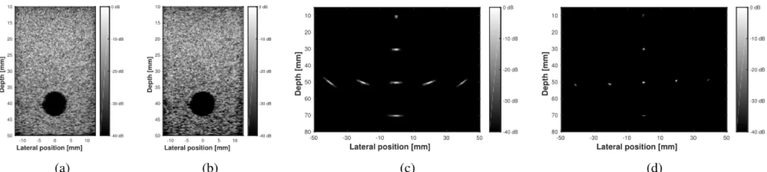
Figures 3a and 3b display the B-mode images of the anechoic-inclusion phantom reconstructed with DAS (11 PW insonifications) and using the proposed approach (1 PW in-sonification), respectively. It can be noticed that the quality is comparable between the two images. The noise inside the anechoic area, due to the side lobes of the PSF, has been suppressed by the regularization. It can also be noticed that the speckle density is slightly decreased with the proposed approach, resulting in a darkening of the image in the deepest part of the Figure 3b. This effect is due to the fact that part of the speckle is not well preserved by the SA model, thus considered as noise and suppressed during the image reconstruction process [14].
B. Reconstruction of the point-reflector phantom
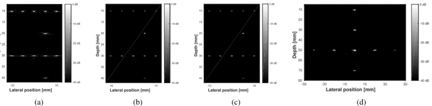
The point-reflector phantom is used to assess the quality of the proposed approach (100 iterations) in the particular case where only few sparse sources are present. One typical application is harmonic imaging of microbubbles in low-concentrations where the individual responses of the sparse microbubbles are visible. The quality is evaluated on the resolution, calculated as the full width at half maximum (FWHM) of the point spread function.
For PW imaging, the proposed approach leads to lateral and axial resolutions of 0.10 mm for every points with 1 PW insonification, while the DAS algorithm gives lateral and axial resolutions of 0.20 mm for both points, constant for compounding experiments with 1 to 11 PW insonifications. The increase is more pronounced in DW imaging where the proposed approach leads to lateral resolutions of 0.50 mm and 0.90 mm and axial resolutions of 0.50 mm for the points located at 30 mm and 50 mm, while the DAS algorithm with 11 DW insonifications exhibits lateral resolutions of 1.40 mm and 2.80 mm and axial resolutions of 0.50 mm.
The increase in resolution is visible when comparing Fig-ures 3c and 3d, which display the B-mode images of the point-reflector phantom reconstructed with DAS (11 DW insonifica-tions) and with the proposed approach (1 DW insonification), respectively.
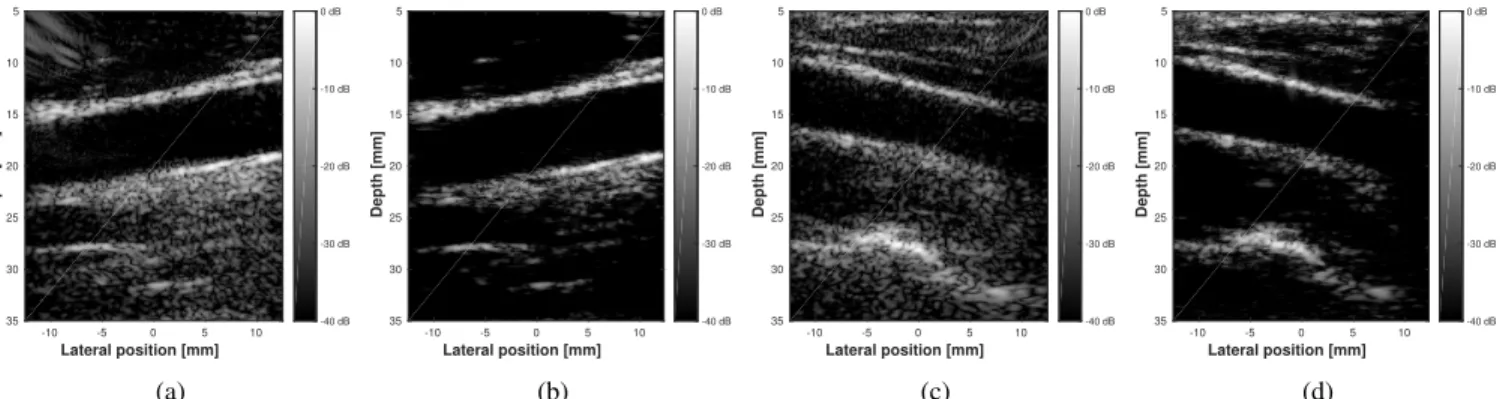
C. Reconstruction of the in vivo carotids
The proposed method is evaluated on the in vivo carotid images. In this case, the SR is coupled with the SA model, the number of iterations is set to 50. Due to the lack of a ground truth image, the evaluation of the image quality is limited to visual assessment.
Figure 4 displays B-mode images for two different carotid acquisitions, reconstructed with the proposed method with 1 PW insonification and using DAS with 9 PW insonifications. It can be observed, by comparing Figure 4a with 4b and Figure 4c with 4d that the proposed method with 1 PW leads to imaging quality similar to DAS with 9 PWs insonifications. Both the anechoic artery and the tissue area are well preserved with the proposed approach.
This illustrates the great potential of SR for reducing the number of insonifications required to reach a given image quality.
D. Reconstruction of the PICMUS dataset
In the above sections, the proposed approach has been compared to DAS. It is now well-known that DAS is not the highest quality beamforming and it could be interesting to compare the proposed approach to the best image reconstruc-tion algorithms.
The proposed method is thus used to reconstruct simu-lated images from the standardized PICMUS dataset [40] and compared against two minimum-variance beamforming approaches [44], [45] and two sparse-based approaches [23], [24]. The results, displayed in Table III, show that the pro-posed method is competitive against the best state-of-the-art
-10 -5 0 5 10 Lateral position [mm] 10 15 20 25 30 35 40 45 50 Depth [mm] -40 dB -30 dB -20 dB -10 dB 0 dB (a) -10 -5 0 5 10 Lateral position [mm] 10 15 20 25 30 35 40 45 50 Depth [mm] -40 dB -30 dB -20 dB -10 dB 0 dB (b) -50 -30 -10 10 30 50 Lateral position [mm] 10 20 30 40 50 60 70 80 Depth [mm] -40 dB -30 dB -20 dB -10 dB 0 dB (c) -50 -30 -10 10 30 50 Lateral position [mm] 10 20 30 40 50 60 70 80 Depth [mm] -40 dB -30 dB -20 dB -10 dB 0 dB (d)
Fig. 3: B-mode images of the anechoic-inclusion phantom reconstructed with (a) DAS for 11 PW insonifications and (b) the proposed approach for 1 PW insonification, and of the point-reflector phantom reconstructed with (c) DAS for 11 DW insonifications and (d) the proposed approach for 1 DW insonification.
-10 -5 0 5 10 Lateral position [mm] 5 10 15 20 25 30 35 40 Depth [mm] -40 dB -30 dB -20 dB -10 dB 0 dB (a) -10 -5 0 5 10 Lateral position [mm] 5 10 15 20 25 30 35 40 Depth [mm] -40 dB -30 dB -20 dB -10 dB 0 dB (b) -10 -5 0 5 10 Lateral position [mm] 5 10 15 20 25 30 35 40 Depth [mm] -40 dB -30 dB -20 dB -10 dB 0 dB (c) -10 -5 0 5 10 Lateral position [mm] 5 10 15 20 25 30 35 40 Depth [mm] -40 dB -30 dB -20 dB -10 dB 0 dB (d)
Fig. 4: B-mode images of two in vivo carotids reconstructed with DAS for 9 PW insonifications ((a) and (c)) and with the proposed approach for 1 PW insonification ((b) and (d)).
-10 0 10 x [mm] 5 10 15 20 25 30 35 40 45 z [mm] -60 -50 -40 -30 -20 -10 0 (a) -10 0 10 x [mm] 5 10 15 20 25 30 35 40 45 z [mm] -60 -50 -40 -30 -20 -10 0 (b) -10 0 10 x [mm] 5 10 15 20 25 30 35 40 45 z [mm] -60 -50 -40 -30 -20 -10 0 (c) -10 0 10 x [mm] 5 10 15 20 25 30 35 40 45 z [mm] -60 -50 -40 -30 -20 -10 0 (d)
Fig. 5: B-mode images of the in vivo carotids of the PICMUS dataset for 1 PW insonification reconstructed with DAS ((a) and (c)) and with the proposed method ((b) and (d)).
approaches in terms of contrast. Regarding the resolution, the method outperforms the other approaches.
The proposed method is lastly used to reconstruct in vivo
carotid images of the PICMUS dataset. The B-mode images, displayed on Figures 5b and 5d show a significant improve-ment compared to DAS, whose corresponding B-mode images are displayed on Figures 5a and 5c, as already demonstrated in Section VI-D. A visual comparison of Figures 5b and 5d against images obtained with best state-of-the-art methods, that one can find on the PICMUS website2, shows that the
2https://www.creatis.insa-lyon.fr/Challenge/IEEE IUS 2016/home
proposed method outperforms most of them in terms of visual quality (in both contrast and resolution).
E. Computation times for sparse regularization
The computation times for the proposed sparse regular-ization method (50 iterations of PDFB) are 119 ms, 164 ms and 163 ms for the cyst phantom, the carotid displayed on Figure 4b and the carotid displayed on Figure 4d respectively. In the case of DW imaging, the point-reflector phantom displayed on Figure 3d is reconstructed in 319 ms.
These timings are two to three orders of magnitude faster than state-of-the-art methods. Indeed, in their latest work,
TABLE III: Comparison of the proposed algorithm against state-of-the-art methods for sparse reconstruction on the sim-ulated PICMUS dataset.
Method Contrast ph. Resolution ph. CNR [dB] Lat. res. [mm] Ax. res. [mm]
DAS 9.96 0.57 0.40 Bessonet al.[23] 15.81 0.15 0.17 Deylamiet al.[45] 17.19 0.08 0.24 Szaszet al.[24] 15.52 0.14 0.11 Varrayet al.[44] 12.65 0.38 0.14 Proposed method 15.71 0.08 0.11
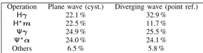
David et al. [46] reported computation times between 3 and 5 min. Szaszet al.[33] reported reconstruction times between 10 s and 1 min. The relative timings of the main operations TABLE IV: Relative timings of the main operations involved in the proposed method for the cyst phantom for PW imaging and the point-reflector phantom for DW imaging.
Operation Plane wave (cyst.) Diverging wave (point ref.)
Hγ 22.1 % 32.9 %
H?m 22.5 % 11.7 %
Ψγ 24.9 % 25.5 %
Ψ?α 24.0 % 24.1 %
Others 6.5 % 5.8 %
involved in the image reconstruction process are reported in Table IV. It can be observed that the timings are balanced between the different operations. It can also be noticed that the computation times of the operations HγandH?m highly
depend on the relative size of the element-raw-data and desired image grids. Indeed, the computation time of the operationHγ
is relatively longer than the one ofH?min the DW case since
the image grid is larger than the element-raw-data grid. It is not the case in the PW case where the two grids are the same.
VI. RESULTS: COMPRESSED BEAMFORMING One issue in US imaging, when analog-to-digital conver-sion (ADC) is carried out in the probe head, is the amount of data that needs to be transferred from the probe to the US system for each insonification. When ADC is carried out in the main system, state-of-the art coaxial cables are not able to embed more than few hundreds coaxial lines, therefore limiting the connections to a few hundreds transducer elements. For probes with a higher number of elements, such as in matrix probes for3D-imaging, time multiplexing is used which may severely impact the frame rate and the range of application. In this section, we explore how the CB framework described in Section III-C could alleviate this bottleneck and benefit the 3D-imaging case.
A. A deep dive into coherence
In order to study US image reconstruction in a CS per-spective, the mutual coherence of the matrix HdΨ, defined
in Section III-C, is evaluated for different sampling strategies and sparsifying bases Ψ. For computational purposes, only 32 transducer elements are simulated and 256 samples are considered in the axial direction with corresponding depth
ranging between 5 mm and 11 mm. The measurement model considered in the study is based on SPW imaging. The coherence is calculated as the maximum non-diagonal value of the Gram matrix of HdΨ [47]. Two different bases Ψ
are evaluated, namely the Dirac basis (Ψis the identity) and the Haar wavelet (Daubechies 1 wavelet) basis, since we are interested in wavelet-based models. Our choice of wavelet basis is limited to Haar wavelet since it is the only one that has a corresponding matrix expression, making the computation of the mutual coherence feasible. Four different sampling strate-gies are compared: uniform selection of transducer elements, random selection of transducer elements, CMIX and CTMIX. Regarding CMIX and CTMIX, the matrixWis generated with coefficients distributed according to normal and Rademacher distributions. For CTMIX, the coherence is evaluated for several values of Dt.
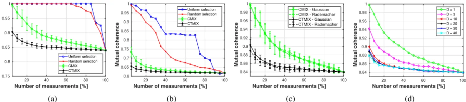
Figures 6a and 6b display the mutual coherenceµ(HdΨ)for
a number of measurements ranging between 5 % and 100 %, whereHd is square in the case of 100 %, withΨbeing Dirac
and Haar bases, respectively. It can be seen that the main benefit of the CMIX and CTMIX strategies reside in their ability to limit the increase of the coherenceµ(HdΨ)induced
by the undersampling of the raw data. In addition, it can be noticed that this effect is more pronounced for the Haar basis than for the Dirac basis. A comparison between CMIX and CTMIX shows that CTMIX has lower coherence than CMIX. This is expected, since CTMIX provides a better mixing than CMIX.
Regarding the impact of the probability distribution of the random coefficients onµ(HdΨ), Figure 6c shows that there is
no significant difference in coherence between Gaussian and Rademacher random coefficients.
Regarding CTMIX, Figure 6d displays the values of
µ(HdΨ) for the different values of Dt. It can be seen that
the mutual coherence decreases when Dt increases. Such a
result is consistent with the theoretical analysis carried out in Section III-C2. For Dt ≥ 10, one may observe that the
coherence values are rather similar. A finer analysis of the coherence for a number of measurements between 0.11 % and 10 % may exhibit the differences in terms of coherence between the values of Dt. However, such high number of
measurements are not considered in the current study.
B. Reconstruction of the point-reflector phantom
The B-mode images, displayed on Figure 7 for PW and DW imaging, show that CB (50 iterations), coupled with CMIX, leads to high-quality reconstruction of point sources even for low numbers of measurements (less than 5 %) for both PW and DW imaging. Two reasons may explain such a result. First, point sources are very sparse, thus well suited to the CS framework. In addition, the measurement matrices associated with CMIX and CTMIX still have a sufficiently low mutual coherence to ensure the perfect recovery condition stated in Theorem 3.1 from [35].
Figure 8 illustrates the peak-signal-to-noise ratio (PSNR) values, calculated on the normalized envelope image (normal-ized means divided by its maximum value), of the different
20 40 60 80 100 Number of measurements [%] 0.75 0.8 0.85 0.9 0.95 1 Mutual coherence Uniform selection Random selection CMIX CTMIX (a) 20 40 60 80 100 Number of measurements [%] 0.6 0.65 0.7 0.75 0.8 0.85 0.9 0.95 1 Mutual coherence Uniform selection Random selection CMIX CTMIX (b) 20 40 60 80 100 Number of measurements [%] 0.84 0.86 0.88 0.9 0.92 0.94 0.96 0.98 1 Mutual coherence CMIX - Gaussian CMIX - Rademacher CTMIX - Gaussian CTMIX - Rademacher (c) 20 40 60 80 100 Number of measurements [%] 0.84 0.86 0.88 0.9 0.92 0.94 0.96 0.98 1 Mutual coherence D = 1 D = 3 D = 10 D = 20 D = 30 D = 40 (d)
Fig. 6: Mutual coherenceµ(HdΨ)against the number of measurements for (a) Dirac basis and (b) Haar basis for the uniform
selection of transducer elements, the random selection of transducer elements, CMIX and CTMIX (Dt=10). Additionally, the
coherence is evaluated (c) for CMIX and CTMIX with mixing coefficients drawn using normal and Rademacher distributions and (d) for CTMIX at different depths.
methods against the reference image, chosen to be the one reconstructed with DAS without data compression.
It can be concluded that CMIX and CTMIX achieve high quality reconstructions for all the considered number of mea-surements. It can also be observed that, in the case of CMIX, the PSNR drops for numbers of measurements lower than 5 % while it remains constant for CTMIX at lower numbers of measurements. Such results are in agreement with the results on the mutual coherence described in Section VI-A.
Regarding the naive strategy where the undersampling cor-responds to the selection of few transducer elements, it can be seen that the PSNR remains high until 10 % measurements and dramatically decreases for lower numbers of measurements. Indeed, because the proposed undersampling strategy is highly coherent, the number of measurements required for perfect reconstruction is higher. Thus, the recovery condition stated by Theorem 3.1 from [35] breaks down for higher numbers of measurements than more incoherent strategies such as CMIX and CTMIX.
C. Reconstruction of the anechoic phantom
The CNR values, summarized in Table V for a number of measurements between 20 % and 50 %, show that CTMIX and CMIX outperform existing strategies. It can also be noticed that CMIX and CTMIX leads to similar results, except at 20 % where CTMIX is superior to CMIX.
One may observe a dramatic decrease of the CNR for 20 % measurements. The same coherence argument as for the point-reflector phantom may be used to explain such a fact. Compared to the point-reflector-phantom, the decrease appears at a noticeably higher number of measurement due to the fact that the anechoic inclusion is less sparse than the point-reflector phantom.
D. Reconstruction of the in vivo carotids
Figures 9b and 9d display the B-mode images of the in vivo carotids obtained with CB (1000 iterations), with 20 % measurements. Figures 9a and 9c display reference images, reconstructed with DAS without data compression. One may notice that textural areas such as carotid plaques and muscle fibers, as well as anechoic areas, are well reconstructed with
TABLE V: CNR values in dB for the three undersampling strategies considered and for different numbers of measure-ments. Method Nb. of measurements 50 % 25 % 20 % Uniform selection 8.81 6.03 0.57 CMIX 9.15 8.06 6.92 CTMIX 9.16 8.10 7.30
TABLE VI: Computation times [ms] of the compressed beam-forming for the three compression strategies (25 % measure-ments) and for the non-compressed case.
Comp. strategy Images cyst. carotid Uniform selection 87 144
CMIX 130 180
CTMIX 212 260
No compression 119 164
CB. However, speckle areas, especially in the far-field, are not well retrieved by the proposed approach, resulting in a darkening of the deepest part of Figures 9b and 9d. This may be explained by the same fact as for SR,i.e.that the wavelet-based models do not preserve well the speckle information, which is thus suppressed during the image reconstruction pro-cess. It can also be noticed that the number of measurements is higher than in the case of the point-reflector phantom. This is directly linked to differences of the image under scrutiny in terms of sparsity.
Figure 10 displays the PSNR values for different numbers of measurements, ranging between 14 % and 50 %. One may observe the same behaviour as for the point-reflector phan-tom. CB achieves a high quality reconstruction even for low numbers of measurements, allowing a drastic reduction in the required number of measurements, for each insonification.
E. Computation times for compressed beamforming
The computation times for the compressed beamforming (50 iterations of PDFB, 25 % measurements) are summarized in Table VI. The proposed methods, as for the sparse regulariza-tion for image enhancement method described in Secregulariza-tion III-B, are three orders of magnitude faster than existing compressed beamforming methods [10]. Regarding the timing of the
-10 10 Lateral position [mm] 10 15 20 25 30 35 40 Depth [mm] -40 dB -30 dB -20 dB -10 dB 0 dB (a) -10 10 Lateral position [mm] 10 15 20 25 30 35 40 Depth [mm] -40 dB -30 dB -20 dB -10 dB 0 dB (b) -10 10 Lateral position [mm] 10 15 20 25 30 35 40 Depth [mm] -40 dB -30 dB -20 dB -10 dB 0 dB (c) -50 -30 -10 10 30 50 Lateral position [mm] 10 20 30 40 50 60 70 80 Depth [mm] -40 dB -30 dB -20 dB -10 dB 0 dB (d)
Fig. 7: B-mode images of the point-reflector phantom for 1 PW insonification ((a) and (b)) and 1 DW insonification ((c) and (d)) reconstructed with DAS ((a) and (c)) and with compressed beamforming coupled with CMIX strategy with 4 % measurements ((b) and (d)). 0 10 20 30 40 50 Number of measurements [%] 34 36 38 40 42 44 46 PSNR [dB] Uniform selection CMIX CTMIX
Fig. 8: PSNR against the number of measurements for the point-reflector phantom insonified with 1 PW for CTMIX, CMIX and the uniform selection of transducer elements.
different strategies, the fastest one is the uniform selection. This makes sense since no additional matrix multiplication is achieved. Regarding CMIX and CTMIX, the multiplication with the random matrix leads to a significant increase of the computation times, which are higher than in the non-compressed case, as shown on Table VI. In addition, the compressed beamforming method coupled with CMIX and CTMIX is no longer matrix-free since the random matrices have to be stored in memory. Thus, the CMIX and CTMIX strategies may be of interest if they come with a simplifica-tion of the hardware, at the cost of a more computasimplifica-tionally demanding reconstruction. These points will be discussed in Section VII-B.
VII. DISCUSSION
A. Towards real-time sparse regularization for enhanced im-age reconstruction
In this work, we have leveraged the problem of memory footprint, which is one of the most challenging aspects in US image reconstruction by SR, as stated in the previous works mentioned in Section I. We have shown that, by exploiting the high parallelization potential of the measurement model, its adjoint and by using fast wavelet transforms [48], the proposed method may achieve image reconstruction two to three orders of magnitude faster than state-of-the-art SR approaches, with
minimal memory requirements. This paves the way to the extension of SR to 3D- imaging, which has not been possible with state-of-the-art methods due to the problem of matrix coefficients storage.
However, the computation times presented in the study are not compatible with real-time imaging yet, mainly due to the computational complexity of the proposed model. The computations time reported in the proposed work are based on a non optimized-code. Thus, one way to accelerate the proposed method consists in optimizing the implementation of the forward model and the adjoint, especially by minimizing the data transfer between the CPU and the GPU. In addition, with the explosion of the computational power of GPUs in the last years, it can be expected that the computation times may be one order of magnitude lower with the next generation of GPUs. Another way towards real-time applications is to lower the number of iterations necessary to reach a given image quality. This can be performed by a better tuning of the hyper-parameters. One recent trend is to consider the use of deep-neural networks in order to tune the hyper-parameters based on a training set. This technique has given very promising results on 1D-signals [49].
The advantage of having a real-time SR is twofold. Firstly, it provides an image enhancement technique, especially for the detection of anechoic area. Secondly, it allows for a reduction of the number of insonifications necessary to reach a given image quality, which is crucial in US imaging application where power supply and power dissipation are problematic,
e.g.in portable systems.
B. Towards compressed sensing in ultrasound imaging
In the proposed work, we suggest innovative sampling schemes for US imaging and thus go one step further to-wards CS in US image reconstruction. Indeed, CMIX and CTMIX strategies outperform existing compression strategies, mainly based on selection of transducer elements, in terms of image quality, as demonstrated in Section VI. However, we face one major obstacle which is the high coherence of the measurement operator. CMIX and CTMIX strategies manage to maintain the coherence constant when the number of measurements is decreased, but the coherence remains high relative to the corresponding Welch bound, because of the
-10 -5 0 5 10 Lateral position [mm] 5 10 15 20 25 30 35 Depth [mm] -40 dB -30 dB -20 dB -10 dB 0 dB (a) -10 -5 0 5 10 Lateral position [mm] 5 10 15 20 25 30 35 Depth [mm] -40 dB -30 dB -20 dB -10 dB 0 dB (b) -10 -5 0 5 10 Lateral position [mm] 5 10 15 20 25 30 35 Depth [mm] -40 dB -30 dB -20 dB -10 dB 0 dB (c) -10 -5 0 5 10 Lateral position [mm] 5 10 15 20 25 30 35 Depth [mm] -40 dB -30 dB -20 dB -10 dB 0 dB (d)
Fig. 9: B-mode images of the in vivo carotids for 1 PW insonification reconstructed with DAS ((a) and (c)) and with the compressed beamforming ((b) and (d)) coupled with the CMIX strategy and 20 % measurements.
10 15 20 25 30 35 40 45 50 Number of measurements [%] 25 26 27 28 29 30 31 32 33 PSNR [dB] Uniform selection CMIX CTMIX
Fig. 10: PSNR against the number of measurements for thein vivo carotid insonified with 1 PW and sampled for CTMIX, CMIX and the uniform selection of transducer elements.
coherence intrinsic to the measurement model. Indeed, the high mutual coherence of the measurement model comes from the fact that each projection onto a 1D-conic, implied by the time-of-flight calculations, involves only a few points in the desired-image space. The natural question that one may ask is whether it is possible to change the nature of the projections in order to involve more points. In fact, this is a relatively difficult task since projections are a consequence of the expression for the round-trip time-of-flight of US waves in a homogeneous medium. This observation has a deep impact on the design of CS acquisition schemes. Indeed, it means that the attempts to decrease the coherence of the measurement model by playing with random pulses sent in transmit is hopeless, because this does not change the expression for the time-of-flight, and thus the fact that echo-samples stem from projections onto 1D-conics.
One solution to this issue may reside in dealing with the coherent operator, by exploring a recent topic on CS, de-noted “constrained adaptive sensing”, which derives sampling theorems and variants of Theorem 3.1 from [35] where the measurement matrix is more constrained than in standard CS [50].
Another alternative could be to entirely rethink the mea-surement process, starting from the requirements of Theorem 3.1 from [35]. Let us consider that we are in a case where the matrixHis random, which is compatible with the requirements of Theorem 3.1 from [35]. In terms of acoustic propagation,
a random measurement model implies that each sample of the element raw-data receives contributions from points spread over the entire image space. In other words, it means that the duality between time and depth, which is at the heart of US imaging, is not valid anymore since echoes from points at different positions reach the transducer elements at the same time. Thus, a random measurement modelHis unfeasible, in pulse-echo imaging in a homogeneous medium, due to the fact that US waves respect the Helmholtz equation. One way to address such an issue resides in placing a scattering or heterogeneous medium in front of the US probe. This principle has been recently developed in optics and gives promising results [51]. However, such a new design raises many questions regarding the choice and the modelling of the heterogeneous medium. It can be easily understood that such a medium may not generate a purely random matrix but will be somewhere in-between a purely random case and the highly coherent case of the homogeneous medium. This topic is currently under study and will be the object of further reports or communications.
C. Limitations of sparsity-driven image reconstruction meth-ods in ultrafast ultrasound imaging
1) The sparsity prior: The first limitation inherent to
it-erative methods lies in the regularization term. Indeed, the prior knowledge on the signal under scrutiny, especially when it comes to imaging living bodies, cannot cover all the cases that one may encounter. Taking that into account, two solutions may be considered.
The first one consists in using analytical models, such as wavelet-based models, which perform well on a wide range of images. This approach is the one we used in this study as well as in our previous work [14]. However, even if wavelet-based models achieve good performance, they tend to decrease the speckle density compared to DAS.
The other alternative consists in using dictionaries, learned on the data by means of dictionary learning algorithms. This has been recently applied to US image reconstruction [21]. At first sight, such a technique appears to be particularly well suited to US imaging. Indeed, US probes are, most of the time, dedicated to one specific application and work at a given frequency. This allows to restrict the size of the training set and facilitates the learning procedure. However, such types
of prior suffer from two major drawbacks. The first one is the risk of overfitting. Indeed, it is a hard task to build a training set of US images whose quality depends on an infinite variety of parameters such as the positioning of the probe, the patient anatomy, etc. In addition, having a sparse prior in a dictionary prevents using fast transforms, which makes its use more difficult in a real-time environment.
2) Sensitivity to the hyper-parameters and data
depen-dency: The efficiency of iterative methods, compared to
analytical approaches, depends on the data that one may want to reconstruct because of the sparsity prior and the hyper-parameters intrinsic to the optimization algorithm. In this work, as well as in previous studies [10], [14], [33], it is firstly shown that SR methods perform well on sparse sources, which make them attractive for harmonic imaging of microbubbles. This can be easily explained by the fact that point sources are very sparse. Secondly, SR methods are efficient for reconstructing images made of structured fibers and anechoic areas such as large vessels, heart cavities, etc. Indeed, such methods manage to remove the noise present in anechoic areas which tends to reinforce the relative intensity of the structured parts. However, these methods struggle when it comes to imaging hyperechoic area. They put too much emphasis on the hyperechoic part to the detriment of the background as described in our previous work [14].
Regarding CB, we observe that, when mixing element raw-data arising from a hyperechoic region embedded in a less echogeneous background, the high intensities of the hyperechoic region tend to interfere with the lower intensity regions, which makes the resolution of the inverse problem very difficult. We also notice that CB is even more sensitive to the sparsity prior and the hyper-parameters than the SR approach used for enhanced image reconstruction, when a mixing is performed. This can be explained by the fact that the inverse problem involving the mixing is more difficult to solve than the one posed by SR for enhanced image reconstruction. One solution to the problem of the hyper-parameters may be to investigate deep-learning approaches, which have been suc-cessfully used to solve sparse-coding problems [52], [49]. The idea consists in mapping one iteration of a convex optimization to one layer of a deep neural network (DNN). The hyper-parameters as well as the non-linearities are learned during the training process of the DNN. The resulting DNN has shown promising results in terms of number of iterations required for convergence and reconstruction quality and is currently under study for the proposed problem. Another solution may consist in investigating in depth the noise induced by the proposed model. While the noise implied by the choice of the proposed model seems to be difficult to quantify, the noised induced by the discretization of the proposed model,i.e.by the interpolation of the continuous integral onto the discrete grid may be studied in depth, in order to identify a lower bound for .
VIII. CONCLUSION
The proposed work presents novel parametric, fast and matrix-free formulations of the measurement model and its
adjoint in the context of ultrafast ultrasound imaging. These formulations are included in a sparse regularization framework which is used to achieve high-quality imaging three orders of magnitude faster than existing methods. By exploiting a sparsity prior of ultrasound images in a model made of a concatenation of wavelets, it outperforms both the delay-and-sum algorithm and the best existing methods, as demonstrated on simulation andin vivoexperiments. In addition, new under-sampling strategies, more suited to compressed sensing than previous ones, are suggested and high quality reconstruction with a low number of measurements are demonstrated. By coupling fast measurement operators suitable for GPU im-plementation with efficient regularization methods, this work paves the way for enhanced ultrafast ultrasound imaging in both 2D and 3D. It also explores, questions and suggests new concepts for the application of CS to ultrasound image reconstruction, based on its fundamental principles.
ACKNOWLEDGMENT
This work was supported in part by the UltrasoundToGo RTD project (no. 20NA21 145911), evaluated by the Swiss NSF and funded by Nano-Tera.ch with Swiss Confederation financing. This work was also supported by the UK Engineer-ing and Physical Sciences Research Council (EPSRC, grants EP/M019306/1). The RF Verasonics system was co-funded by the FEDER program, Saint-Etienne Metropole (SME) and Conseil General de la Loire (CG42) within the framework of the SonoCardio-Protection Project lead by Prof. Pierre Croisille. The authors would also like to thank Dr Olivier Bernard from CREATIS laboratory for providing the in vivo
acquisition data.
APPENDIXA: DERIVATION OF THE PARAMETRIC EQUATIONS FOR A STEERED PLANE WAVE AND A
DIVERGING WAVE
Let us remind the forward problem defined in Equation (8):
h(xt, t) = Z r∈Γ(xt,t) od(r, xt)γ(r) | ∇rg| dσ(r), (28) in whichg(r, xt, t) =t−tT x(r)−tRx(r, xt), andΓ (xt, t) = {r∈Ω|g(r, xt, t) = 0}.
A. Steered plane waves
Let us consider a SPW with angle θ. As shown by Mon-taldo et al. [41], the propagation delay in transmit can be written as: tT x(x, z) = x−x? t c sinθ+ z c cosθ, (29)
wherex?t is the position of the transducer element which emits
According to Equation (29), the following equivalence holds: r= [x, z]T ∈Γ (xt, t) ⇔ q (x−xt) 2 +z2+ (x−x? t) sinθ+zcosθ=ct ⇔(ct−(x−x?t) sinθ−zcosθ)2−(x−xt)2−z2= 0 ⇔Az2+Bz+C= 0 ⇔z=−B± √ ∆ 2A . (30)
where∆ =B2−4AC andA,B andC are defined by:
A =−sin2θ,
B = 2 (x−x?
t) cosθsinθ−2ctcosθ,
C = (ct−(x−x?t) sinθ)2−(x−xt) 2
.
(31) In the specific case where A = 0, i.e. in the case where
θ= 0, the parametric equation can be directly expressed as:
z(x, xt, t) = 1 2ct (ct)2−(x−xt) 2 . (32) B. Diverging waves
Let us consider a DW with a virtual point source located at [xn, zn]
T
. As demonstrated by Papadacci et al. [42], the propagation delay in transmit can be written as:
tT x(x, z) = q (x−xn)2+ (z−zn)2−d0, (33) whered0= min xt q (xn−xt) 2 +z2 n.
According to Equation (33), the following equivalence holds: r= [x, z]T ∈Γ (xt, t) ⇔4(x−xn)2+ (z−zn)2 (x−xt)2+z2 = (ct+d0) 2 −(x−xn) 2 −(z−zn) 2 −(x−xt) 2 −z2 2 ⇔(A+z)2=B ⇔z=−A±√B, (34) where A=−zn 2 1 + (xt−x) 2 −(xn−x) 2 (d0+ct)2−zn2 ! , (35) and B = (d0+ct) 2 4z2 n−(d0+ct) 22 (xt−xn)2+zn2−(d0+ct)2 (xt+xn)2+zn2−(d0+ct)2−4x(xt+xn−x) . (36)
APPENDIXB: DETAILED MATRIX-FREE FORMULATIONS OF THE MEASUREMENT MODEL AND ITS ADJOINT
A. Measurement model
Let us remind Equation (9):
h(xt, t) = Z x∈R od(x, z(x, xt, t), xt) | ∇(x,z(x,xt,t))g| γ(x, z(x, xt, t))|Jz(x)|dx. (37)
If we consider the image grid defined in Section II-A and the interpolating kernelϕ: R→R, then, according to [53],
γ(x, z(x, xt, t))can be expressed as:
γ(x, z(x, xt, t)) = Nz X q=1 ϕ(zq−z(x, xt, t))γ(x, zq) +νϕ(z(x, xt, t),z), (38)
where νϕ(z(x, xt, t),z) ∈ R accounts for the interpolation
error. The discretization of Equation (9) leads to the following formulation: h(xt, t) = Nx X n=1 od(xn, z(xn, xt, t), xt)|Jz(xn)| | ∇(xn,z(xn,xt,t))g| Nz X q=1 ϕ(zq−z(xn, xt, t))γ(xn, zq) +νϕ(z(xn, xt, t), zq). (39)
To end up with the complete formulation of the measure-ment model, we deduce from Equation (7) that m(xt, t) = (h(xt)∗tvpe) (t), where∗tdenotes the 1D-discrete
convolu-tion, which can be easily implemented “on-the-fly”.
Thus, the element-raw data are related to the TRF samples by the following operator:
H(γ, xt, t) =νϕ0 (xt, t) + Nt X l=1 vpe t−tl Nx X n=1 od xn, z xn, xt, tl , xt |Jz(xn)| | ∇(xn,z(xn,x t,tl))g| Nz X q=1 ϕ zq−z xn, xt, tl γ(xn, zq), (40)
which can be computed “on-the-fly” and in parallel for each point of the element-raw-data grid and in which νϕ0 (xt, t) is
the overall error defined by:
νϕ0 (xt, t) = Nt X l=1 vpe t−tl Nx,Nz P n=1,q=1 od(xn,z(xn,xt,tl),xt)|Jz(xn)| |∇(xn ,z(xn ,xt,tl))g| νϕ z x n, x t, tl , zq. (41)
Thus, by evaluating Equation (40) for each point(xjt, tl)of
the element-raw-data grid, the following relationship holds:
mxjt, tl =Hγ, xjt, tl +νϕ0 xjt, tl , (42)
which defines Equation (10) by taking into account the other sources of noise (model and measure).
B. Adjoint operator of the measurement model
The adjoint operator of the measurement model is defined in Equation (11) as: ˆ γ(r) = Z xt∈Ξ od(r, xt) (m(xt)∗tu) (tT x(r) +tRx(r, xt))dxt. (43)
If we set t(r, xt) = tT x(r) +tRx(r, xt), we consider the
element-raw data grid defined in Section II-A and the inter-polating kernel ϕ:R→R, then, similarly to Equation (38), m(xt, t(r, xt))can be expressed as:
m(xt, t(r, xt)) = Nt X l=1 ϕ t(r, xt)−tlm xt, tl +ξϕ(t(r, xt),t), (44)
whereξϕ(t(r, xt),t)∈Raccounts for the interpolation error.
The discretization of Equation (11) leads to the following formulation: H?(m,r) =ξ0 ϕ(r) + Nt X l=1 u tl Nel X j=1 od r, xjt Nt X s=1 ϕtr, xjt−tl−tsmxjt, ts, (45)
which can be computed “on-the-fly” and in parallel for each point of the image grid and in which ξϕ0 (r) =
Nt,Nel,Nt P l=1,j=1,s=1 u tlod r, xjt ξϕ tr, xjt −tl, ts.
Thus, by evaluating Equation (45) for each point (xn, zq)
of the image grid, the following relationship holds:
γ(xn, zq) =H?(m, xn, zq) +ξ0
ϕ(xn, zq), (46)
which defines Equation (12) by taking into account the other sources of noise (model and measure).
APPENDIXC: ADJOINT OPERATOR OF THE CONTINUOUS MEASUREMENT MODEL
The continuous measurement model, defined in Equa-tion (2), can be written as:
m(xt, t) =T {γ}(xt, t), (47)
whereL2(Ω)designates the space of square integrable
func-tions with values in Ω and T : L2(Ω) → L2(Ξ×R) is a
functional described by: T {γ}(xt, t) =
Z
r∈Ω
γ(r)od(r, xt)
vpe(t−tT x(r)−tRx(r, xt))dr. (48)
In order to define the adjoint of the operator T, let us introduce a function n ∈ L2(Ξ×R). The inner product
betweenT {γ} andn can be written as:
<T {γ}, n >=
Z Z
xt∈Ξ,t∈R
T {γ}(xt, t)n(xt, t)dxtdt, (49)
which can be expressed as:
<T {γ}, n >= Z Z r∈Ω,xt∈Ξ γ(r)od(r, xt) Z t∈R n(xt, t)vpe(t−tT x(r)−tRx(r, xt))dxtdtdr. (50)
Let us now focus on the integral over the variabletwhich can be formulated as: Z t∈R n(xt, t)vpe(t−tT x(r)−tRx(r, xt))dxtdt = Z t∈R n(xt, t)u(tT x(r) +tRx(r, xt)−t)dxtdt = (n(xt)∗tu) (tT x(r) +tRx(r, xt)), (51)
whereu(t) =vpe(−t)is the matched filter of the pulse-echo
waveform.
This leads to the following expression for the inner product:
<T {γ}, n >= Z r∈Ω γ(r) Z xt∈Ξ od(r, xt) (n(xt)∗tu) (tT x(r) +tRx(r, xt))dxtdr. (52)
Let us define the operatorT? from Equation (52) as:
T?{n}(r) =
Z
xt∈Ξ
od(r, xt)
(n(xt)∗tu) (tT x(r) +tRx(r, xt))dxt. (53)
IntroducingT? in Equation (52) leads us to the following
equality:
<T {γ}, n >=< γ,T?{n}>, (54)
which defines the adjoint operator ofT.
APPENDIXD: PRIMAL-DUAL-FORWARD-BACKWARD ALGORITHM
The general problem we solve, which can be seen as an instance of Problem (12) of [34], is the following one:
min
x∈CN
f1(x) +f2(Φx−y), (55)
given the assumption that f1 :CN →R and f2 : CM → R
are lower semicontinuous convex functions.
The key mathematical tool used in PDFB is the proximity operator of a convex function defined as:
proxf(x) = arg min
z∈CM
f(z) +1
2kz−xk 2
2. (56)
In the proposed `1-minimization problem f1(x) = k؆xk1
andf2(x) =iB(x), whereiB is the indicator function of the