Evolution of Spiking Neural Networks
for Temporal Pattern Recognition and
Animat Control.
Author:
Ahmed Abdelmotaleb
A thesis submitted to the University of Hertfordshire in partial fulfilment of the requirements for the degree of Doctor of Philosophy
Evolution of Spiking Neural Networks for Temporal Pattern Recognition and Animat Control.
I extended an artificial life platform called GReaNs (the name stands for Gene Regu-latory evolving artificial Networks) to explore the evolutionary abilities of biologically inspired Spiking Neural Network (SNN) model. The encoding of SNNs in GReaNs was inspired by the encoding of gene regulatory networks.
As proof-of-principle, I used GReaNs to evolve SNNs to obtain a network with an output neuron which generates a predefined spike train in response to a specific input.
Temporal pattern recognition was one of the main tasks during my studies. It is widely believed that nervous systems of biological organisms use temporal patterns of inputs to encode information. The learning technique used for temporal pattern recognition is not clear yet. I studied the ability to evolve spiking networks with different numbers of interneurons in the absence and the presence of noise to recognize predefined temporal patterns of inputs. Results showed, that in the presence of noise, it was possible to evolve successful networks. However, the networks with only one interneuron were not robust to noise.
The foraging behaviour of many small animals depends mainly on their olfactory sys-tem. I explored whether it was possible to evolve SNNs able to control an agent to find food particles on 2-dimensional maps. Using firing rate encoding to encode the sensory information in the olfactory input neurons, I managed to obtain SNNs able to control an agent that could detect the position of the food particles and move toward it. Furthermore, I did unsuccessful attempts to use GReaNs to evolve an SNN able to con-trol an agent able to collect sound sources from one type out of several sound types. Each sound type is represented as a pattern of different frequencies.
In order to use the computational power of neuromorphic hardware, I integrated GRe-aNs with the SpiNNaker hardware system. Only the simulation part was carried out using SpiNNaker, but the rest steps of the genetic algorithm were done with GReaNs.
I am using this opportunity to express my gratitude to everyone who supported me throughout my PhD study, specially my supervisors: Borys Wr´obel, Maria Schilstra, Neil Davey, and Volker Steuber. I would like also to thank my parents for their support and my sister Noha for her help. Special thanks to my fianc´ee Ceyna for encouraging and supporting me. I am also grateful to my friend Adam Peszke for helping me in reviewing the English of my thesis, and to Micha l Joachimczak for his help in debugging GReaNs.
The work presented in chapter 8 in this thesis was done in collaboration with Dr. Sergio Davis from University of Manchester. This work was done during CapoCaccia workshops in 2012, 2013, and 2014. I received a scholarship from Convergent Science Network of Biomimetic and Biohybrid Systems (CSN) to attend Capocaccia 2012 workshop. During Capocaccia 2013 and 2014 workshops, I was supported by both University of Hertfordshire and Foundation for Polish Science.
I would like to thank Artur Jarmolowski and Arleta Kucz from Adam Mickiewicz Uni-versity in Poznan for their support and help for maintaining the logistical issues during my stay in Poland.
I used the PhD thesis of Nicolas Oros as a reference for me to follow the standard of PhD thesis of University of Hertfordshire as he was a previous PhD student there. I used a latex template to shape up this thesis. I downloaded this template from http://www.latextemplates.com. The authors of this template are Steven Gunn and
Sunil Patel. The license of this templatee can be foundhere.
I usedSharelatex online latex editor for my thesis which allowed me to share the thesis with my supervisors easily.
My work was supported by Adam Mickiewicz University in Poznan, Poland, by the Polish National Science Centre (projects BIOEMERGE, UMO-2011/03/B/ST6/00399, and EvoSN, UMO-2013/08/M/ST6/00922, both awarded to Dr. Borys Wr´obel), and by the International PhD Programme ”From Genome to Phenotype: A Multidisciplinary Approach to Functional Genomics” (awarded by the Foundation for Polish Science, co-financed by EU Regional Development Fund—Innovative Economy Operational Pro-gramme 2007-2013) at the Adam Mickiewicz University.
Abstract ii
Acknowledgements iii
Contents iv
List of Figures viii
List of Tables xii
1 Introduction 1
1.1 Motivation and Goals . . . 1
1.2 Contribution to Knowledge . . . 2
1.3 Structure of the Thesis . . . 4
1.3.1 Chapter 2 . . . 4 1.3.2 Chapter 3 . . . 4 1.3.3 Chapter 4 . . . 5 1.3.4 Chapter 5 . . . 5 1.3.5 Chapter 6 . . . 6 1.3.6 Chapter 7 . . . 6 1.3.7 Chapter 8 . . . 6 2 Literature Review 7 2.1 Central Nervous System . . . 7
2.2 Neuron. . . 8
2.3 Spiking Neural Networks . . . 9
2.3.1 Leaky Integrate-and-Fire neural model . . . 11
2.3.2 Non-Linear Integrate-and-Fire models . . . 12
2.3.3 Hodgkin and Huxley model . . . 14
2.3.4 Simulation of Spiking Neural Networks. . . 15
2.4 Neural coding . . . 16
2.4.1 Rate code . . . 16
2.4.2 Population rate code . . . 17
2.4.3 Binary code . . . 17
2.4.4 Latency code . . . 17
2.4.5 Rank order code . . . 18
2.5 Temporal Pattern Recognition with Spiking Neural Networks . . . 18
2.5.1 Introduction . . . 18
2.5.2 Encoding and decoding mechanism for Temporal Pattern Recog-nition . . . 19
2.5.3 Training SNNs for Temporal Pattern Recognition. . . 19
2.6 Animat Foraging with Spiking Neural Networks . . . 21
2.6.1 Introduction . . . 21
2.6.2 The model . . . 22
2.6.3 The agent . . . 22
2.6.4 The environment . . . 24
2.6.5 Encoding strategies for the sensory information . . . 25
2.6.6 Adding noise to the neural network. . . 26
2.7 Genetic Algorithm . . . 27
2.8 Gene Regulatory Network . . . 28
3 Mapping GRNs to SNNs in GReaNs platform 30 3.1 Introduction. . . 30
3.2 From genome to network. . . 30
3.3 Evolution of networks in GReaNs . . . 33
3.4 Mapping the GRN to the SNN . . . 34
3.4.1 LIF Model in GReaNs . . . 35
3.4.2 AdEx Model in GReaNs . . . 36
3.4.3 Validating the SNN implementation in GReaNs . . . 37
3.5 The Evolution of the SNN . . . 38
3.6 Conclusion . . . 38
4 Using GreaNs to Evolve a Spiking Neural Network which Generates Desired Spike Patterns 40 4.1 Introduction. . . 40
4.2 Genetic algorithm . . . 41
4.3 Results. . . 43
4.3.1 Reproducing spike trains . . . 43
4.3.2 Double-shifting task . . . 44
4.4 Conclusion . . . 48
5 Temporal Pattern Recognition in GReaNs 49 5.1 Introduction. . . 49
5.2 Genetic algorithm . . . 50
5.3 Temporal pattern recognition with a sequence of four inputs. . . 50
5.4 Temporal pattern recognition with a sequence of three inputs . . . 52
5.4.1 Pattern 1-2-3 recognition with a varying hard-coded limit on the size of the network . . . 52
5.4.2 The robustness to temporal noise . . . 55
5.4.3 Network analysis . . . 56
5.4.3.1 Category 1 . . . 57
5.4.3.2 Category 2 . . . 60
5.5 Conclusion . . . 64
6 Real Time Control of Foraging Behaviours 65 6.1 Introduction. . . 65
6.2 The Model . . . 66
6.2.1 Spiking Neural Networks Model. . . 66
6.2.2 Animat Simulation . . . 66
6.2.3 Genetic algorithm . . . 68
6.3 Encoding sensory information in the SNNs in GReaNs . . . 70
6.3.1 The strength of food smell at sensors to synaptic conductance injection . . . 70
6.3.2 Unary coding . . . 77
6.3.2.1 Using the (V −Vth) thrust . . . 77
6.3.2.2 Using the constant thrust . . . 82
6.3.2.3 Using the sliding window thrust . . . 85
6.3.3 Encoding the sensory information at sensors as current injection . 90 6.4 Conclusion . . . 99
7 Temporal Pattern Recognition in Animats 101 7.1 Introduction. . . 101
7.1.1 The description of the animat and its simulation environment . . . 102
7.1.2 Genetic algorithm . . . 103
7.1.3 Results for this task . . . 103
7.1.4 Using two sound source types . . . 104
7.2 Conclusion . . . 108
8 Integrating GReaNs with SpiNNaker 109 8.1 Introduction. . . 109
8.2 The integration model . . . 110
8.3 Results. . . 111
8.3.1 Initial communication protocol with the small SpiNNaker board . 111 8.3.2 Communication protocol with the big SpiNNaker board . . . 113
8.4 Conclusion . . . 114
9 General Conclusion and Future Work 116 9.1 General Conclusion . . . 116
9.2 Future Work . . . 118
9.2.1 SNNs model and the evolutionary algorithm. . . 118
9.2.2 Temporal pattern recognition . . . 118
9.2.3 Evolving SNNs for animat control . . . 119
Bibliography 121
2.1 A simplified structure of a biological neuron. . . 8
2.2 A schematic diagram for a spike generated by a neuron. . . 9
2.3 An example of a synapse between two neurons. . . 10
2.4 The first generation model of an artificial neuron . . . 10
2.5 An example of a spike generated by a neuron. . . 11
2.6 Schematic diagram of the LIF model . . . 12
2.7 An example of an AdEx neuron behaviour. . . 13
2.8 The difference between count, latency, and rank coding schemes for 10 neurons over a time window of 10 ms . . . 16
2.9 Hopfield decoding mechanism for temporal pattern recognition . . . 20
2.10 The structure of the Natschl¨ager and Ruf network . . . 21
2.11 The agent model used by Oros and colleagues . . . 23
2.12 The representation of chemicals in the model presented by Oros and col-leagues . . . 24
2.13 The relation between the concentration of chemicals at the antennae and the firing rate of the sensory neurons in the model presented by Oros and colleagues . . . 25
2.14 The relation between the concentration of the chemicals and the firing rate of the sensory neurons using sigmoid function in the model presented by Oros and colleagues . . . 26
2.15 The behaviour of the animat before and after adding the colored noise in the model presented by Oros and colleagues . . . 28
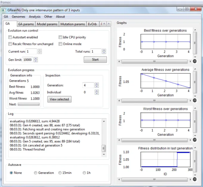
3.1 A screenshot of the initial window of GReaNs software . . . 31
3.2 The structure of the genome in GReaNs . . . 32
3.3 How edges between nodes in the GRN are created in GReaNs . . . 33
3.4 The relation between the affinity of the connection between any promoter and any gene in the genome and the β factor in GReaNs . . . 33
3.5 A simple model to test the behaviour of SNNs in GReaNs . . . 38
3.6 The difference between the behaviour of a simple SNN using both GReaNs and Brian simulator . . . 39
4.1 The behaviour of the champion networks evolved to match a response of a single neuron, but shifted with 5 ms . . . 43
4.2 The behaviour of the champion networks evolved to match a response of a single neuron, but shifted with 10 ms. . . 44
4.3 The behaviour of the champion networks evolved to match a response of a single neuron, but shifted with 20 ms. . . 44
4.4 The behaviour of the champion networks evolved to match a response of a single neuron, but doubled and shifted with 5 ms . . . 45
4.5 The behaviour of the best LIF network (in terms of generalization) to match the spikes of single AdEx neuron shifted by 20 ms. . . 47
4.6 The behaviour of the best LIF network (in terms of generalization) to match the spikes of single AdEx neuron shifted by 5 ms. . . 47
4.7 The behaviour of the best AdEx network (in terms of generalization out of 10 independent evolutionary runs) evolved to double-shift the spikes of single LIF neuron. . . 48
5.1 The evolved SNN to distinguish one pattern of four inputs . . . 52
5.2 The behaviour of the evolved SNN to distinguish the pattern 1-2-3-4 . . . 53
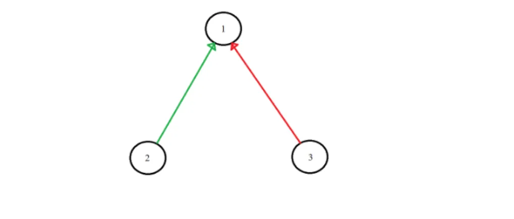
5.3 The evolved SNN with one interneuron to distinguish one pattern of three inputs . . . 54
5.4 The evolved SNN with two interneurons to distinguish one pattern of three inputs . . . 55
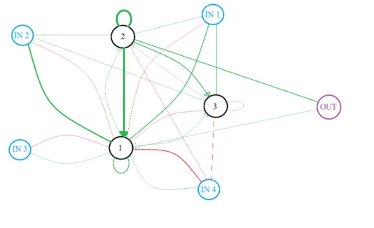
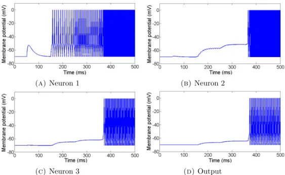
5.5 A SNN from category 1 with three inputs and two interneurons robust to noise with sd 10 ms. . . 59
5.6 A SNN from category 2 with three inputs and two interneurons robust to noise with sd 10ms . . . 61
5.7 A SNN from category 3 with three inputs and two interneurons robust to noise with sd 10ms . . . 63
6.1 The model of the animat evolved in order to collect targets on 2D maps. . 67
6.2 The gradation of the strength of food smell generated by 20 targets in GReaNs . . . 68
6.3 A suboptimal behaviour of the agent that has been discovered before when the GRN was used in GReaNs. . . 70
6.4 The behaviour of the animat that had been evolved using simulation time 2 s and synaptic conductance injection coding when it was simulated for 2 s . . . 72
6.5 The behaviour of the animat evolved using simulation time 10 s and synaptic conductance injection coding when it was simulated for 10 s . . . 73
6.6 The behaviour of the evolved animat using synaptic conductance injection coding using simulation time 6 s during the evolution when simulated for 10 s . . . 74
6.7 The behaviour of the best evolved animat using synaptic conductance injection coding using simulation time 6 s during the evolution . . . 75
6.8 The evolution history of the best animat evolved using conductance in-jection coding . . . 75
6.9 The behaviour of the best evolved animat using unary coding using sim-ulation time 6 s . . . 78
6.10 The evolution history of the best animat evolved using unary coding . . . 78
6.11 The right and the forward thrusts generated by the actuators during the simulation of the best animat evolved using unary coding and (V −Vth)
thrust with 1 target on the map. . . 80
6.12 The right and the forward thrusts generated by the actuators during the simulation of the best animat evolved using unary coding and (V −Vth)
6.13 The behaviour of the evolved animat using unary coding and constant thrust using simulation time 6 s . . . 82
6.14 The behaviour of the evolved animat using unary coding and constant thrust using simulation time 12 s . . . 83
6.15 The right and the forward thrusts generated by the actuators during the simulation of the best animat evolved using unary coding and constant thrust with 1 target on the map. . . 84
6.16 The right and the forward thrusts generated by the actuators during the simulation of the best animat evolved using unary coding and constant thrust with 20 targets on the map. . . 85
6.17 The behaviour of the best evolved animat using unary coding and sliding window thrust using simulation time 6 s . . . 86
6.18 The behaviour of the best evolved animat using unary coding and sliding window thrust using simulation time 12 s . . . 87
6.19 The right and the forward thrusts generated by the actuators during the simulation of the best animat evolved using unary coding and sliding window thrust with 1 target on the map. . . 88
6.20 The right and the forward thrusts generated by the actuators during the simulation of the best animat evolved using unary coding and sliding window thrust with 20 targets on the map. . . 89
6.21 The relation between the strength of smell at the sensors and the injected current at the input neurons using the Hill function (Equation 6.10) using a step period 1 ms. . . 91
6.22 The relation between the strength of smell at the sensors and the firing rate of the input neurons using the Hill function (Equation 6.10) using a step period 1 ms. . . 91
6.23 The relation between the injected current at the inputs and the firing rate of the input neurons using the Hill function (Equation 6.10) using a step period 1 ms. . . 92
6.24 The relation between the strength of smell at the sensors and the injected current at the input neurons using the Hill function (Equation 6.10) after decreasing the step period to 25 µm. . . 92
6.25 The relation between the strength of smell at the sensors and the firing rate of the input neurons using the Hill function (Equation 6.10) after decreasing the step period to 25 µm. . . 92
6.26 The relation between the injected current at the inputs and the firing rate of the input neurons using the Hill function (Equation 6.10) after decreasing the step period to 25 µm. . . 93
6.27 The difference between the animat before and after modifications . . . 93
6.28 The difference between the strength of smell at the right sensor and the left sensor before increasing the radius of the animat and the length of the sensors and after increasing the radius of the animat and the length of the sensors . . . 93
6.29 The behaviour of the best evolved animat using current injection coding after 1000 generations on a map for 6 targets. . . 95
6.30 The evolution history of the best animat evolved using current injection coding . . . 95
6.31 The behaviour of the best evolved animat using current injection coding after 1100 generations . . . 96
6.32 The behaviour of the best animat after re-evaluation using current injec-tion coding simulated for 3 s . . . 97
6.33 The behaviour of the best animat after re-evaluation using current injec-tion coding simulated for 30 s . . . 98
7.1 A simplified description of the task of collecting sound sources. . . 102
7.2 The evolution history of the evolved animat to collect sound sources with pattern 1-2-3 and ignore sound sources with other five patterns . . . 104
7.3 The evolution history of the best animat in the population to collect sound sources with pattern 1-2 and ignore sound sources with pattern 2-1 . . . . 105
7.4 The behaviour of the evolved animat when the sound sources with the first pattern were presented . . . 106
7.5 The behaviour of the evolved animat when the sound sources with the second pattern were presented. . . 107
8.1 The communication protocol between GReaNs and SpiNNaker . . . 111
8.2 The distribution of the neurons of the 300 SNNs over SpiNNaker board . 112
8.3 The small SpiNNaker board with only 4 chips which was used in the first version of the integration . . . 113
8.4 The big SpiNNaker board with 48 chips which was used in the second version of the integration . . . 115
3.1 Mapping the Gene Regulatory Network to Spiking Neural Network in GReaNs . . . 35
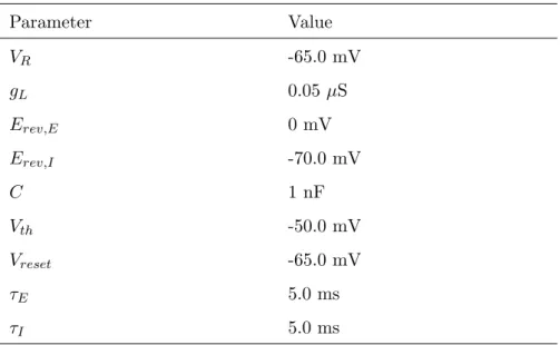
3.2 LIF model parameters values . . . 36
3.3 AdEx model parameters values . . . 37
4.1 Statistics on the behaviour of the best networks of 10 independent evolu-tionary runs . . . 46
4.2 Comparison between the networks with the best ferr values during the
evolution and the networks with the best ferr values for generalization
over the 10 independent evolutionary runs. The numbers out side the parentheses are the values offerr during the evolution while the numbers
in the parentheses are the values offerr for generalization . . . 46
5.1 Evolution of robustness to noise in a temporal pattern recognition task in LIF networks with 1 interneuron . . . 56
5.2 Evolution of robustness to noise in a temporal pattern recognition task in LIF networks with 2 interneurons . . . 56
5.3 Evolution of robustness to noise in a temporal pattern recognition task in LIF networks with 5 interneurons . . . 57
5.4 Evolution of robustness to noise in a temporal pattern recognition task in LIF networks with 10 interneurons. . . 57
Introduction
1.1
Motivation and Goals
The work I have carried out during my PhD is part of broader research program to compare the computational properties of Spiking Neural Networks (SNNs) and networks that are not spiking. At the beginning of my studies, I built two SNN models: Leaky Integrate and Fire model (LIF) [1, 2] and Adaptive exponential leaky integrate and fire model (AdEx) [3] based on the previous Gene Regulatory Networks (GRNs) that have been implemented before in the artificial life platform GReaNs (the name stands for Gene Regulatory evolving artificial Networks) [4]. Mapping the GRNs to SNNs in GReaNs allowed me to use theem genetic algorithm which was already implemented before in GReaNs and used for GRNs.
Researchers showed that the brain uses temporal patterns of spikes to encode sensory information [3, 5–11]. It has been shown that temporal coding is used in vision [5], hearing [12], and olfaction [13] (more details in 2.5.1). The exact learning mechanism the brain uses for training the neurons to recognize temporal pattern is not clear yet. Hopfield [14] presented a mechanism for encoding and decoding temporal patterns of spikes. This mechanism is based on the delays of the synapses of the input neurons and a coincidence detection mechanism. Based on Hopfield’s work, some studies have been done in training the delays of the input neurons synapses for temporal pattern recognition [15–18].
In contrast, I developed a learning algorithm that is based on evolving only the weights and the topology of the networks using fixed delays for the synapses. After successfully obtaining SNNs able to recognize some patterns of inputs, I investigated the behaviour of these networks and checked their robustness when noisy patterns were used for testing.
The foraging system of many animals depends on the olfactory sensory neurons that allow collecting information about the odours in the environment [19, 20]. Moths for example have a strong olfactory system on which their foraging system depend. These tiny animals with very small brain have the ability to locate chemical sources even if they are miles away from them [19, 20]. The exact way how the sensory information is encoded in animal’s brain and how these sensory information is transferred for actions is not clear yet.
During my PhD studies, I investigated the different ways of encoding the sensory infor-mation in spiking neural networks and the different ways of updating the forces at the actuators based on these sensory information.
The ability of using SNNs for animat foraging was also investigated in previous work [21–25]. GReaNs platform was used before for evolving GRNs able to control animats for food foraging [26,27]. Using the same genetic algorithm, I evolved SNNs in GReaNs to control animats for collecting food particles in 2D environment and compare their behaviour with the behaviour of the animats when GRNs were evolved.
Being able to explore the tasks of temporal pattern recognition and animat foraging in GReaNs opened the gate for me to investigate more interesting tasks by merging both tasks together. I replaced the food particles in the food foraging task with sound sources. Each sound source is represented with number of input neurons each with different frequency.
SpiNNaker [28] (Spiking Neural Network Architecture) is a massively parallel computing system which was designed to support large scale spiking neural networks simulations. I was interested in using the computational power of SpiNNaker with GReaNs. I inte-grated SpiNNaker with GReaNs so that the simulation step of the evolutionary algorithm is done with SpiNNaker and the rest of the steps are carried out using GReaNs.
1.2
Contribution to Knowledge
My main contribution to knowledge has been to extend the range of behaviour of spiking neural network models. In particular I show how the inherently temporal behaviour of a spiking neural network can be used in both the decoding of temporally coded information and in the production of temporal behaviour. This has been shown in the more detailed contributions described below:
1. I have created a biologically inspired Spiking Neural Network (SNN) model to al-low the evolution of the topology of the SNNs and the weights of their synapses. I
build this model based on Gene Regulatory Network model which was implemented before in GReaNs platform. I used two popular SNN models in my work: Leaky integrate and fire model (LIF) and Adaptive exponential leaky integrate and fire model (AdEx) SNN models. Using genetic algorithm, I evolved the SNN to ac-complish number of tasks including generating a predefined spike train in response to specific input, temporal pattern recognition, animat foraging, and temporal pattern recognition with animats.
2. The first main evolutionary task I have carried out during my PhD studies was evolving SNNs able to perform temporal pattern recognition. I have introduced an evolutionary algorithm based on evolving only the topology of the network and the weights of the synapses between the neurons in the network. Learning algorithms have been used before in order to obtain SNNs able to perform temporal pattern recognition [15–18]. These algorithms were based on adjusting only the delays between the neurons in the SNNs. I have used networks with various numbers of interneurons (1, 2, 5, and 10) and I compared their robustness to Gaussian noise with various standard deviation (10, 20, and 30 ms) added to the spike times of the inputs. Furthermore, I studied the different behaviours of the SNNs of two interneurons which are robust to noise and found that the positive feedback loops are important for robustness of the SNNs to noise.
3. I evolved SNNs which were able to control animats in order to perform food for-aging. I have introduced various coding strategies for the sensory information represented the concentration of the food. I have also investigated three different ways of determining the thrusts at the actuators of the animats. After using these coding strategies and the ways of determining the thrusts, I compared the evolved animats based on some factors. These factors include the ability of the evolved animat to cope with high food density when it was simulated on a map which contained large numbers of targets.
4. I have investigated the ability to evolve spiking neural networks in order to control an animat able to detect and distinguish between temporal patterns emitted by simulated sound sources. The animat was supposed to effectively discriminate between different sequences of simulated acoustic signals, measure the distance to the sound source, and move towards a desired source. Althought it was not possible to evolve this animat successfully, I presented some suggestions that could lead in the future work to have an animat that could successfully do this task.
5. I have integrated the GReaNs evolutionary software with SpiNNaker system [28] in order to use its computational power to simulate large scale SNNs. The idea was to run the simulation part in the genetic algorithm with SpiNNaker while the
other steps of the genetic algorithm were carried out with GReaNs. I have used two evolutionary tasks for the integration each with different SpiNNaker board. Although the integration did not afford any improvement, this work can be seen as a contribution to theory by presenting a communication protocol between an evolutionary algorithm and a neuromorphic hardware. I also suggested some ideas in order so speed up the integration between GReaNs and SpiNNaker.
1.3
Structure of the Thesis
The structure of the thesis is the following:
1.3.1 Chapter 2
This chapter presents the literature review I have done during my PhD studies. At the beginning of the chapter, I introduced briefly the different neural networks from the first, second, and third generations. Then I explained two models of artificial neurons commonly used in SNN research and which I used in my work (Leaky Integrate and Fire (LIF) [1, 2] and Adaptive exponential leaky integrate and fire model (AdEx) [3, 29]). Later in this chapter, I presented various neural coding and how sensory and motor information can be represented in the brain using spikes.
The main two tasks I carried out during my PhD studies were evolving SNNs for temporal pattern recognition and animat foraging. In the last part of the chapter, I reviewed the work that have been done previously in these two tasks.
1.3.2 Chapter 3
The third chapter describes the GReaNs platform. This platform was used before to evolve gene regulatory networks (GRN) to perform some tasks including controlling mul-ticellular development in three dimensions [30–32], processing signals [33] and controlling animats [26,27].
At the beginning of the chapter I describe how the GRN is constructed from the genome and the steps of the genetic algorithm which is used to evolve the GRNs. The third chapter includes also a description for the first task I carried on during my PhD study of mapping the GRN in GReaNs to spiking neural network (SNN). In this task I im-plemented two different SNN models, Leaky Integrate and Fire model (LIF) [2] and Adaptive exponential leaky integrate and fire model (AdEx) [3,29].
Finally I validated the behaviour of a simple SNN in GReaNs by comparing its behaviour with the behaviour of the same SNN simulated using PyNN package [34] with Brian simulator [35] as a back-end simulator.
1.3.3 Chapter 4
This chapter presents the first evolutionary task I have tried in GReaNs after mapping the GRN to SNN successfully. This task includes evolving SNNs to obtain a network able to generate a predefined spike train in response to specific input. This task can be divided to two main parts. First, obtain LIF (or AdEx) SNN able to generate the same spike train (shifted by 5ms, 10ms, or 20ms) generated by a single AdEx (or LIF) neuron when both the SNN and the single neuron are connected to the same input.
The second part consists of obtaining LIF (or AdEx) SNN able to double (generate two spikes 5 ms and 25 ms after each spike) the spike train generated by a single AdEx (or LIF) neuron when both the SNN and the single neuron are connected to the same input. Finally, I tested the generalization of the final networks obtained from the previous two sub-tasks by comparing the behaviour of the single neuron and the evolved SNN when both of them are connected to a different input other than the one which was used during the evolution.
1.3.4 Chapter 5
The temporal pattern recognition task which is one of the two main tasks I did during my studies is presented in this chapter. In this chapter I studied the ability to evolve spiking networks, with varying numbers of LIF neurons (1, 2, 5, 10, and unlimited) to recognize predefined temporal patterns of different number of inputs (3 and 4). Then I tested the behaviour of the final networks when Gaussian noise with different standard deviations (10, 20, and 30 ms) was applied to the time of the spike in each input. Furthermore, I used the noisy inputs during the evolution and checked if I could get final networks without error. It was interesting then to study the difference between the structure of the final networks (with only 2 interneurons) which were evolved in absence of noise and the final networks (with 2 interneurons also) which were evolved with presence of noise.
1.3.5 Chapter 6
After evolving SNNs for generating predefined spike trains and for temporal pattern recognition, I explored a more practical task that is relevant for evolutionary robotics. This task includes evolving SNNs for real time control of foraging behaviours. This task is introduced in this chapter. First, I introduce the the model I used of the animat and the description of the simulation environment; this includes the structure of the animat and the food resources on the map. The next section describes the genetic algorithm used in this task.
One of the most important issues covered in this chapter is the various strategies of encoding the sensory information in the SNN. Finally, I introduce the results and discuss about the methods I applied in order to improve the behaviour of the animat.
1.3.6 Chapter 7
This chapter presents the description of the integration of the temporal pattern recogni-tion task and the real time control of foraging behaviours task. The descriprecogni-tion includes the structure of the animat, and the simulation environment. Finally, I introduce the results of the experiments and discuss these results.
1.3.7 Chapter 8
The integration work I have done with SpiNNaker [28] (SpikingNeuralNetworkArchitecture) is presented in this chapter. SpiNNaker is a massively parallel computing system. Due to its high computational power, it can afford real-time simulation for a large scale SNNs with thousands of neurons. In this chapter, I introduce two versions of integration I have done with two different SpiNNaker boards.
In the first version, the task of evolving LIF SNNs to match the spike train of a single AdEx neuron shifted by 5 ms described in chapter 4 was presented using the small SpiN-Naker board with only four chips. In the second version, I used the bigger SpiNSpiN-Naker board with 48 chips to integrate with GReaNs. The task of evolving SNNs with 10 interneurons for temporal pattern recognition in the presence of noise was explored in this version. Finally, I compare in terms of computational time the results of the two tasks with the results of the same tasks when SpiNNaker boards were not used.
Literature Review
2.1
Central Nervous System
The nervous system is responsible for controlling all the body parts and for commu-nications between them. The nervous system consists of two main parts, the central nervous system which includes the brain and the spinal cord and the peripheral nervous system which includes sensory and motor neurons responsible for connecting the central nervous system with all body parts and the environment.
The spinal cord is a long and thin bundle of nervous tissue that resides in the vertebral cavity. It is responsible for a large part of the communication between the brain and the rest of the body. On the other hand, the brain, which resides in the head, is considered the most complex organ in the human body. It is responsible mainly for processing and analysing the information it receives from the sensory neurons located in the peripheral nervous system and taking decision based on it. Most of the actual information processing takes place in the cerebral cortex which plays a very important rule in consciousness, memory, attention, perception, and language.
The structure and the function of the brain have been studied by many experimentalists and theoretical neurobiologists over the past hundred years. These studies showed that the size of the brain varies a lot between animals. African elephant brain contains 257 billion neurons which makes it the animal with the largest counted number of neurons [36]. Most of the neurons in the elephant brain are located in the cerebellum [36]. Sperm whale brain is about two times larger than elephant brain, but the exact number of neurons in the whale brain is not known yet. On the other hand, the predatory rotifer Asplanchna brightwellii brain contains only 200 neurons [37].
Human brain has around 80 billions [38] of neurons (Fig. 2.1). These neurons are considered the elementary processing units in the nervous system [39]. Neurons connect to each other in an efficient way to process the incoming signals in order to make decisions and control movements. Neurons communicate with each other with short electrical pulses.
2.2
Neuron
Fig. 2.1 shows the biological neuron: for a simplified view, each neuron receives most of the incoming signals through their dendrites, these signals change the voltage (also called membrane potential) of this neuron. When the voltage reaches the value of the threshold, the neuron generates a spike or an action potential which is sent to the connected neurons through the axon. The effect of the presynaptic neurons on the postsynaptic neurons depends mainly on the type of the presynaptic neuron (excitatory or inhibitory) and the strength of the synapses between them.
Figure 2.1: A simplified structure of a biological neuron. At the middle of the cell body of the neuron resides the nucleus which contains the genetic material. Each neuron receives input spikes from other neurons through its dendrites and cell body. At the output stage, the neuron uses its axon to send spikes to all connected neurons. From
http://webspace.ship.edu/cgboer/theneuron.html.
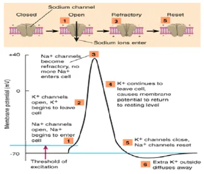
The action potential (Fig. 2.2) generated by a neuron is a fast depolarization resulted from opening of the two ion channels (sodium Na+ and potassium K+) of the neuron. When the membrane potential reaches the maximum value, the membrane is repolarized
until the potential reaches the minimum value during the refractory period in which the neuron cannot fires more spikes.
Figure 2.2: A schematic diagram for a spike generated by a neuron. When
the membrane potential of a neuron reaches the threshold (1), its ion channels open leading for membrane depolarization (2). When the membrane potential reaches the maximum value (3), the membrane is repolarized and the potential decreases till it reaches the rest potential (5). The potential continue decreas-ing until it reaches the minimum value durdecreas-ing the repfractory period (6). From
http://www.bazaarmodel.net/Onderwerpen/neuron/ps2lec1.htm.
The spike is transferred from the presynaptic neuron to the postsynaptic neuron through the synapse between the two neurons. The synapse (Fig. 2.3) is a microscopic gap that lies between the axon of the presynaptic neuron and the dendrites of the postsynaptic neuron. A series of chemical events occur during the transferring of the signal through the synapse. These events include releasing of neurotransmitters (chemical substances) from the presynaptic neuron and receiving them by receptor sites in the postsynaptic neuron.
2.3
Spiking Neural Networks
Modeling neural systems has passed a number of generations of research, starting from McCulloch-Pitts threshold neurons [40] which are considered the first generation of ar-tificial neural networks. This model simply considers the neuron as a digital element which sends a binary signal if the sum of the incoming signals, scaled by their weights,
Figure 2.3: An example of a synapse between two neurons. The transfer of the spike from the axon of the presynaptic neuron (upper part) to the dendrite of the postsynaptic neuron (lower part) includes transmission of neurotransmitters to the posysynaptic
receptors. From http://www.bazaarmodel.net/Onderwerpen/neuron/ps2lec1.htm.
crosses the value of the threshold (Fig. 2.4). This model have been applied on many artificial neural networks, for example, multi-layer perceptrons and Hopfield networks [41].
McCulloch-Pitts’s model has been modified in the second generation by replacing the threshold by a continuous activation function (usually sigmoid or hyperbolic tangent [42]) which allows for analog inputs and outputs. The output of the neuron in this network lies in the range [0, 1] when the sigmoid function is used while it lies in the range [-1, 1] when the hyperbolic function is used. Second generation neural networks are considered more powerful as they can be used for analog input and output.
Figure 2.4: The first generation model of an artificial neuron. In this model the neuron
works as a digital element which sends a binary signal if the sum of the incoming signals (x1, ..., xn), scaled by their weights (w1, ..., wn), crosses the value of the threshold (θ).
The use of spikes (Fig. 2.5) appeared in the third generation of neural models, which is considered even more biologically realistic. Using spikes allows the model neurons in these spiking neural networks (SNNs) [39,44–46] to communicate with each other using single pulses like real neurons. This facilitates the representation of time in the model.
Figure 2.5: An example of a spike generated by a neuron. The neuron receives
inputs from the connected neurons (x1, ..., x4) which allows the membrane potential to
integrate until it reaches the threshold voltage when the neuron fires a spike. After firing a spike the membrane potential is set to the reset voltage. The neuron needs to wait for a period of time until it can fire another spike (refractory period). Taken from http://lis2.epfl.ch/CompletedResearchProjects/EvolutionOfAdaptiveSpikingCircuits/.
2.3.1 Leaky Integrate-and-Fire neural model
The Leaky Integrate-and-Fire (LIF) model [1, 2] is the simplest and most widely used spiking neuron model. In this model, a neuron is represented by a basic electrical circuit (Fig. 2.6). As we can see in the circuit on the right-hand side, an input current I(t) charges a capacitor and flows across a resistor, which are arranged in parallel.
I(t) =I(C) +I(R) (2.1)
whereI(C) is the current which charges the capacitor, andI(R) is the current through the resistor. From Ohm’s law:
I(R) = V
R (2.2)
whereV is the voltage over the resistor. From the definition of the capacity:
I(C) =CdV
dt (2.3)
I(t) = V(t)
R +C
dV
dt (2.4)
We can introduce a new constant called membrane time constant:
τm=RC (2.5)
then we can write the previous equation as following:
τmdV
dt =−V(t) +RI(t) (2.6)
which is the general equation of the membrane potential in the LIF model. When the membrane voltage of a neuron reaches the value of thresholdθ, the neuron generates a spike, and the value of the membrane potential is reset toVr. Often, a short refractory period where the neuron is unresponsive is included by clamping the membrane potential toVr for the duration of a few milliseconds.
Figure 2.6: Schematic diagram of the LIF model. On the left side, a presynaptic
spike arrives at the synapse. A low-pass filter is used to convert the pulseδ to input current I(t). On the right side, the basic circuit of the neuron which shows the current I(t) charges the RC circuit. If the voltage crosses the value ofθ at time t(if), a spike
δ(t−t(if)) is fired. Taken from [43].
2.3.2 Non-Linear Integrate-and-Fire models
The LIF model is too simple to produce many behaviours observed in real neurons. For example, behaviours that are not captured by standard LIF models include bursting and spike rate adaptation, that is, the gradual reduction of spike rate over time. Adding
an adaptation variable and a non-linearity can make Integrate-and-Fire models more biologically realistic. The adaptation variable allows for the production of spiking and bursting behaviour of known types of cortical neurons (regular spiking, adapting, delayed spike initiation, bursting, initial bursting, and fast spiking) [47]. The general equations of such models are as following:
dV
dt =F(V)−w+I (2.7)
dw
dt =a(bV −w) (2.8)
wherewis the adaptation variable, a and b are constants, and the functionF(V) varies from model to model.
• Adaptive Exponential (AdEx) LIF Model [3,29] is one of the non-linear integrate-and-fire models that uses an exponential function (for exampleexp(V−Vt
δ ) whereV
is the membrane potential,Vtis the threshold potential, andδis the slope factor).
Both the membrane voltage V and the adaptation variable w are reset when the neuron fires a spike (Fig. 2.7).
Figure 2.7: The temporal evolution of the membrane potential (top) and the
adap-tation variable (bottom) in an AdEx model. When the AdEx neuron fires a spike, the value of the adaptation variable is increased by a constant value which decreases the
• Izhikevich model [48] is also considered non-linear integrate-and-fie model. This model uses a quadratic function (xV2+yV+z, whereV is the membrane potential and x,y, and zare constants) forF(V) in Equ. 2.7.
2.3.3 Hodgkin and Huxley model
In 1952, Alan Lloyd Hodgkin and Andrew Huxley presented a neural model when they performed some experiments on the giant axon of the squid [49–53]. Their model is based on three different ionic currents, sodium (Na), potassium (K), and a leak current (L). These ionic currents charge the capacitor as following:
CdV
dt =−ΣjIt(j) +I(t) (2.9)
where C is the capacitance, V is the membrane potential, ΣjIt(j) is the sum of the
current from all the ionic channels, and I(t) is the injected current.
The current from all the ionic channels (ΣjIt(j)) can be calculated using the following
equation:
ΣjIt(j) =gN am3h(V −EN a) +gKn4(V −EK) +gL(V −EL) (2.10)
wheregN a,gK,gLare constanct conductances,EN a,EK,ELare reversal potentials, and
m, n, and h are called gating variables which are used for activation and deactivation and caclulated using following equations:
dm dt =αmV(1−m)−βmV m (2.11) dn dt =αnV(1−n)−βnV n (2.12) dh dt =αhV(1−h)−βhV h (2.13)
whereα and β are voltage dependent rate constants.
The Hodgkin and Huxley model is not suitable for large number of neurons simulation and for real time simulations as it is very expensive model to implement. To evaluate 0.1
ms of model time using Hodgkin and Huxley model, it takes 120 floating point operations [54].
On the other hand, adaptive leaky integrate and fire models (AdEx and Izhikevich models) allow to adequately simulate the behaviour of cortical neurons [54].
I used only LIF and AdEx models during my studies as both of them are supported in SpiNNaker [28] system with which I was planning to integrate my work.
2.3.4 Simulation of Spiking Neural Networks
Simulating SNNs is a field that attracted many researchers and engineers. Many software tools have been implemented for simulating SNNs on personal computers. These tools include the simulators Brian [35], Nest [55], and Neuron [56].
Dedicated hardware systems have been also used for SNN simulation. Hardware sim-ulators can provide real time simulations of SNNs and consume less energy. Based on the approach used for the implementation of the neural models, the hardware simula-tors can be divided into analog (for example, Neurogrid [57]) and digital (for example, SpiNNaker [28]) hardware simulators.
Analog hardware simulators consume less energy and take less area. It has been shown [58] that analog simulators consume 20 times less energy than digital simulators while they take 5 times area less than digital simulators. On the other hand, the digital hardware simulators are less noisy which make them not sensitive to process variability. Using all of these software and hardware tools will require writing different scripts for each tool to define the structure and the settings of the SNNs. To make the simulation of SNNs on different simulation tools, PyNN [34] has been developed. PyNN is a simulator-independent platform for building neuronal network models. Using PyNN, the network structure can be described in the Python programming language. PyNN also allows choosing which simulator back-end to be used during the simulation. Both software simulators and hardware simulators can be used as a back-end simulator for PyNN.
2.4
Neural coding
The previous section provided a brief overview about some types of neuronal models, and gave examples of simple spiking neuron models that can be used to study the spike-based representation of information in neural networks. The current section explores how sensory and motor information can be represented in the brain using spikes. This work was presented originally in [59].
2.4.1 Rate code
A firing rate code is the simplest and most commonly used form of information trans-mission between neurons. This model is based on considering the sensory neurons as analog-to-frequency converters as the intensity of the stimulus is mapped onto the firing rate, with high stimulus intensity mapped onto high firing rate and low intensity mapped onto low firing rate [59].
Figure 2.8: The difference between count, latency, and rank coding schemes for 10
neurons over a time window of 10 ms. Each neuron can generate only one spike. In this simple example, there are (10 + 1) possible states with a count code, while by using a latency code we can get 1010states. Finally, there are 10! possible states using a rank
2.4.2 Population rate code
This code is a special case of a rate code that is based on counting the number of spikes generated by a number of neurons during a specific time window. The advantage of a population rate code compared to a rate code that relies on a single neuron is that the time window that is required to count spikes is smaller. Fig. 2.8illustrates a population rate code (here called count code) that operates based on a single spike per neuron. In this particular example there are nine spikes generated during a window of 10 ms, so the population frequency of this population of N = 10 neurons is 90s−1. In order to compare this code with other codes, the amount of data (in bits) that can be represented by this code will be calculated by taking the logarithmic value with base 2 of the possible number of states that can be represented with each code. There are (N + 1) possible states for the count code of this population during this window (from 0 toN spikes). In which means that the maximum amount of data that can be transferred using this code islog2(N+ 1) bits.
2.4.3 Binary code
During the observation window, each neuron could either fire one spike or keep silent, so each neuron could be seen as a line in a ten-line digital cable. As we can see in Fig. 2.8, the current state of the population could be described by the binary sequence 1111111101, and the total amount of information that could be transmitted would be
log2(210) bits or in general forN neuronslog2(2N) bits.
2.4.4 Latency code
The latency or timing code is one of the most efficient codes as it is based on the precise timing of the spikes of each neuron. The middle column in Fig. 2.8 shows the latency code of each neuron. Since the observing window is 10 ms, the latency code can take any of the values from 1 to 10 or null. The amount of information that can be transmitted using this code depends on the precision of the determination of the time of each spike. Using a precision of 1 ms, the maximum amount of information that could be transmitted in the observation window (t) is log2(t)N bits, whereN is the number of
neurons. However, although efficient, latency codes are very sensitive to temporal noise in the spike trains.
For a population of neurons, the relative latency code of each of them can be interpret the spiking patterns generated by this population.
2.4.5 Rank order code
Instead of looking at the exact timing of the spikes, this code is based on the order in which the neurons fire spikes, thereby addressing the problem of the sensitivity of a latency code to noise. For the population in Fig. 2.8 the order C-B-D-A-E-F-G-J-H-I is transmitted. There are N! different orders that can be generated by N neurons which makes the total amount of information that could be transferred usingN neurons
log2(N!) bits.
2.5
Temporal Pattern Recognition with Spiking Neural
Networks
2.5.1 Introduction
In the 20th century, it was widely believed that neurons in the brain use firing rate (described in 2.2.1) to encode their sensory information (for example, [60, 61]). One of the early and leading studies in neural coding showed that there is a strong relation between the firing rate of the stretch receptor neurons in the muscles and the force applied to the muscle [62,63]. Based on these studies, the firing rate coding was used to describe the properties of different sensory neurons in response to various actions. It was used to describe the modality and topographical attributes of cat’s cortex neurons in response to different actions including movement of hairs and pressure upon the skin [60]. Moreover, the firing rate was used to describe the properties of anesthetized cat’s cortical neurons in response to stimulating its retina separately or simultaneously with light spots of various sizes and shapes [61].
By the end of the 20th century, many studies have been made criticizing the ability of firing rate to encode all sensory information. Temporal pattern code was presented as an alternative [3,5–11]. For example, one of these studies [5] criticized the ability of the firing rate coding to be used in the movement-sensitive neuron in the visual system of the blowfly. The reason behind that is that the course correction of the blowfly takes only 30 ms while the firing rate of the movement-sensitive neuron is in the range between 100 to 200s−1. This constraint limits the number of spikes generated by the movement-sensitive neurons during the course correction of the blowfly to an extent that makes using firing rate code not appropriate.
Other studies [9] proposed that cortical neurons use more than one form of neural coding. For single neurons both firing rate code and temporal structure of the spike trains are used. For large population of neurons, both the population coding and the
temporal coding can be used. As I mentioned in the previous section, the population code is considered a special case of the firing rate code which involves counting the spikes generated by a population of neurons. The coordinated-coding uses the relationship between the signals from the neurons in this population to represent the messages in the cortical neurons. This relationship could be the order of the spikes generated by each neuron in the population.
Thorpe and colleagues argued that human brain can recognize 3D objects in less than 400 ms which makes it impossible for the straight forward firing rate code to be used for processing information for vision without using the exact time of spikes [64]. Fur-thermore, it has been shown that temporal coding is used for processing information for hearing [12] and olfaction [13].
2.5.2 Encoding and decoding mechanism for Temporal Pattern
Recog-nition
As we explored in the previous section that it is widely accepted that the brain uses temporal pattern of inputs to encode sensory information. Hopfield suggested an encod-ing and decodencod-ing mechanism for temporal pattern recognition [14]. His mechanism was based on the synaptic delays of the inputs with the temporal patterns, then detecting the coincidences between these inputs (Fig. 2.9). He suggested that radial basis function can be used by the decoding neurons for recognizing specific temporal patterns.
2.5.3 Training SNNs for Temporal Pattern Recognition
Delays play a crucial rule in the mechanism suggested by Hopfield. If his mechanism is true, then there must be a learning mechanism for these delays in the brain. Natschl¨ager and Ruf have suggested a structure of a Spiking Neural Networks used for temporal pattern recognition [15]. They also proposed a learning algorithm for the synaptic delays that allows obtaining a network able to differentiate between different temporal patterns.
The network Natschl¨ager and Ruf have presented (Fig. 2.10) contains two layers. The input neuron layer contains all the inputs of the network (u1 to um). Each input (ui)
fires only one spike at timexi during a total interval T. The second layer is the output
layers which contains the output neurons (v1 to vn). Since the main job of the output
neurons is to calculate a radial basis function (RBF), output neurons are called RBF neurons.
Figure 2.9: Hopfield decoding mechanism. The mechanism that was suggested by
Hopfield includes two aspects. First, each of the synapse between the inputs and the decoding neuron has delay, then coincidences of the input patterns is detected using radial basis function (RBF) in the decoding neuron which is called RBF neuron. Taken
from [65]
RBF neuron is a neuron that spikes only if it observes the same input pattern that the neuron was encoded with.
Each input neurons is connected with RBF neuron by a synapses with weight wij and delaydij. If the spikes from all input neurons arrive at any RBF neuron at the same time,
this will let the RBF neurons fire a spike which will inhibit the other RBF neurons before this RBF neuron inhibits itself. Natschl¨ager and Ruf have used leaky-integrate-and-fire model to model the RBF neurons.
Natschl¨ager and Ruf used an unsupervised learning algorithm for the RBF neurons to be able to cluster input patterns. The idea of their algorithm is to allow each input neuron ui to be connected with each RBF neuron vj with multiple synapses each with different weight wij(k) and delay d(ijk). The values of the weights and delays are initially chosen randomly from predefined ranges. Each RBF neurons vj should receive at least one spike from all inputs before it spikes. The idea of the algorithm is that each RBF neuron rewards the synapses which drive it to spike and punish the other synapses. The rewarding and punishment mechanism is performed by allowing each RBF neuron to propagate spikes back through its synapses when it fires a spike. Based on the differ-ence between the presynaptic and postsynaptc spikes times each synapse is rewarded (punished) by increasing (decreasing) the synaptic weight respectively. In case that the
Figure 2.10: The structure of Natschl¨ager and Ruf network. Each input neuronui
is connected with each output neuronvj by a synapse with weight wij and delay dij.
When the output neuron fires a spike it inhibits the other output neurons and then it inhibits itself.Taken from [15]
difference between the presynaptic and postsynaptc spikes times is small, the synapse is rewarded and vise verse.
Steuber and colleagues also showed that decoding of temporal parallel fibre input pat-terns can be implemented in a multi-compartmental model of a cerebellar Purkinje cell [16–18,66]. They used a non-hebbian learning algorithm for training the synaptic delays between the neurons in the network. They used a biochemical mechanism for adapting the synaptic delays. Adapting the synaptic delay was modelled by adapting the latencies of calcium responses after activation of metabotropic glutamate receptors.
2.6
Animat Foraging with Spiking Neural Networks
2.6.1 Introduction
Many animals depend on their olfactory system for foraging [19]. The foraging system relies on the olfactory sensory neurons to collect information about odours in the en-vironment. The information collected by the sensory neurons is encoded as spikes and sent to the brain through the axons of the sensory neurons [67]. Many coding strategies have been proposed in the olfactory system to encode the information collected from the environment. These coding strategies include the firing rate, the number of the active
sensory neurons and the synchronization of firing between the sensory neurons [19]. Re-cently, Oros and collaborators have investigated the ability of evolving SNNs to control animats for foraging [22]. In the following sections I will cover in more detail the work by Oros and colleagues on controlling agents.
2.6.2 The model
A network of simple LIF models was used to control the agent. In this model the membrane potential of every neuron was updated every time step (0.1 ms was used) based on the following equation:
dV dt =− V τm + n X j=1 IjWj (2.14)
where V is the membrane potential of the neuron, τm is the membrane time constant, nis the number of synapses, Ij is the current received from synapse numberj, and Wj
is the weight of this synapse (in units of 1/F). During the experiments, the value of the membrane time constant (τm) was set to 50 ms.
The resting potential was set to 0 mV, the thresholdθwas set to 20 mV, and a refractory period of 3 ms was used. After a neuron fires a spike, the synaptic current of all postsynaptic target neurons is given by the following equation:
Ij(t) = t−(tspike+delay) τs exp 1−(t−(tspike+delay)) τs (2.15)
where tspike is the time when the presynaptic neuron fired the spike, delay is the con-duction delay between the neuron which fired the spike and the neuron which received it, and τs is the synaptic time constant. The synaptic time constant (τs) was set to 2
ms. The delay is calculated with the following function:
delay=coef fdelay×distance (2.16)
wherecoef fdelay is the delay coefficient anddistanceis the distance between the neuron which fired the spike and the neuron which received it. coef fdelay = 5×10⁻⁵ was used.
2.6.3 The agent
Oros and colleagues used an agent similar to a Braitenberg vehicle [68]. In this model (Fig. 2.11) the agent has two wheels, one on the right side and one on the left side;
each of them is controlled by two motor neurons. Each wheel can move forward or backward. One motor neuron supports forward movement and another motor neuron supports backward movement.
On the front of the agent, there are two antennae. Each of these antennae is connected to a sensory neuron. The distance between the two antennae was long enough in order to allow a large difference in the chemical concentration. In the absence of any chemical concentration, the agent will be still be able to move forward thanks to adding a baseline input current (0.5 A/F) to the forward motor neurons. Every 10ms, the velocity of the agent is updated by calculating the difference between the firing rate of the forward motor neurons and the backward motor neurons as following:
Vw =Kv Sf orward−Sbackward tperiod (2.17)
whereVw is the velocity of each wheel, Kv is a constant,tperiod is the period after which
the velocity was updated, Sf orward is the number of spikes fired by the forward motor
neuron duringtperiod andSbackward is the number of spikes fired by the backward motor
neuron during the same period tperiod. Kv = 0.3 and tperiod = 10ms were used during the experiments.
Figure 2.11: The agent model used by Oros and colleagues. Two long antennae
(black) were connected to sensors (yellow) in order to detect the chemicals and two wheels controlled by 4 neurons 2 of them were responsible for forward movement (green) and the other 2 were responsible for the backward movement (orange). The numbers
2.6.4 The environment
Oros and colleagues used a 2-dimensional map to simulate the world. Only two chemi-cals were placed on the map. Each chemical was represented as a circle of concentration where the maximum concentration is at the centre of the circle and the concentration gradually decreases with the distance from the centre (Fig. 2.12).
Figure 2.12: The representation of chemicals in the model presented by Oros and
colleagues. The chemical is represented as a circle where the maximum concentration is at the centre of the circle, and it linearly decreases when we move far from the centre.
Taken from [25].
The concentration of each chemical can be calculated at any place on the map using the following equation:
c=max((M ax−(K×d)),0) (2.18)
wherecis the concentration at any place on the map,M axis the maximum concentration (at the center of the chemical),K is a constant anddis the distance between the center of the chemical and the place where the concentration is calculated. M ax= 300 andK
2.6.5 Encoding strategies for the sensory information
Oros and colleagues showed that the agent could use both temporal coincidence and firing rate encoding strategies depending on the level of concentration of the chemical at the antennae. When the network used the firing rate encoding only, the agent was not able to detect the difference of the chemical concentration between its two sensors for low concentrations. The network used temporal coincidence encoding for low concentration. With high chemical concentrations, the firing rate encoding was working well.
For the firing rate encoding, choosing the suitable equation to map the concentration of chemicals to sensory neuron current was the main concern for Oros and colleagues. As we can see in Fig. 2.11, the two antennae are connected with 2 sensory neurons. Based on the concentration of the chemical read at the antennae, the sensory neuron current is calculated. The membrane potential is updated every time step based on the sensory neuron current and when the membrane potential reaches the threshold θ, the sensory neuron fires a spike. This leads to an indirect relation between the concentration of the chemical at the antennae and the firing rate of the sensory neuron connected to this antennae (Fig. 2.13).
Figure 2.13: The relation between the concentration of chemicals at the antennae and the firing rate of the sensory neurons in the model presented by Oros and colleagues.
Take from [23].
In order to obtain a model able to detect the small differences between the concentration of the chemicals between the right and left antennae it was very important to find a suitable function to map the chemical concentration to sensory neuron current so that there would be linear relation between the concentration and the firing rate of the sensory neuron. Oros and colleagues tried many equations to map the concentration at the antennae to sensory neuron current [23]. First they started by setting a linear relation between the concentration and the current but the firing rate of the sensory neurons was saturating. They also tried to use Hill function to map the concentration
to the sensory neuron current. Hill function was first used by Archibald Hill in 1910 for describing the binding of oxygen to Hemoglobin.
Using the Hill function they got a better relation between the concentration and the firing rate of the sensory neurons but it was not linear yet. Finally they used a sigmoid function with offset. The equation they used was as following:
I =K1× 1 1 +exp h−C K2 +b (2.19)
where I is the current, K1, K2, h, and b are constants, and C is the concentration. K1 = 3.9∗104, K2 = 59, h =691, and b = 0.08 were used. The relation between the
concentration and the firing rate (Fig. 2.14) was not exactly linear, but it was still accepted.
Figure 2.14: The relation between the concentration of the chemicals and the firing
rate of the sensory neurons using sigmoid function in the model presented by Oros and colleagues. Taken from [23].
2.6.6 Adding noise to the neural network
Oros and collaborators noticed that the agent moved straight through and then away from the chemical source when the agent trajectory was directly along the direction of the gradient of the chemical concentration. In this case the values of the concentration of the chemical were equal at the two antennae and the agent could not recognize the position of the chemical source. They added noise to the neural network in order to overcome this problem [21]. Diffusive Ornstein-Uhlenbeck current noise [69] was added to the equation of the total current (Eqn. 2.15). The noise current was calculated as following: dI(t) dt =− 1 τI (I(t)−I0) + s 2σ2 τI ξ(t) (2.20)
where I is the total current, τI is the current noise time constant (2ms in their case),
I0 is the mean synaptic current (0 in their case),σ is the noise diffusion coefficient and ξ(t) is a white Gaussian noise (with mean = 0 and standard deviation = 1). Different values ofσ were used in the experiments in the range of [0, 0.001].
Adding this coloured noise mimicked the subthreshold voltage fluctuations in real neu-rons due to the intense network activity [70]. After implementing this noise, the agent was able to stay in the range of the chemical concentration (Fig. 2.15).
In the work I present in Chapter 6 and Chapter 7, I built on the work that had been done by Oros and colleagues. I used the Hill function they used in order to map the food concentration at the sensors to input current.
My work can be considered an extension to the work I have just presented in this chapter. In the work done by Oros and colleagues, they used only one food source from the same type. I allowed the environment to have more food sources (up to 20 food sources), and when the animats ate one of these food sources, this food source disappeared and the concentration map was updated. This task is considered more difficult as the animat should be able to deal with different levels of concentrations.
One of the main extensions I have also done was upgrading the food sources to sound sources. Each sound source produces a different temporal pattern of sounds. The animat should distinguish between them and be able to move forward to only one sound source with a specific pattern.
The differences and the similarities between my work and the work that had been done by Oros and colleagues are presented in more details in chapter 6.
2.7
Genetic Algorithm
The genetic algorithm (GA) is one of the heuristic search algorithms which was invented by John Holland in the 1960s [71]. It was inspired by the evolution theory of Darwin (survival of the fittest) and is well described in many books [72–76]. It is an example of the evolutionary algorithms which uses natural evolution techniques for searching opti-mal solution. These techniques include inheritance, mutation, selection, and crossover. In nature, crossover occurs in the reproduction process of the chromosomes in which genes from parent chromosomes recombine together to produce new chromosomes. An-other operation which also happens during reproduction of chromosomes is mutation. Mutations happen by applying some changes in the produced chromosomes. Fitness is another term that is used as a measurement of how good a solution is. It is kind of
Figure 2.15: The behaviour of the animat before and after adding the colored noise in the model presented by Oros and colleagues. After running the agent for 300s, the agent (red path) was not able to stay in the range of the chemical concentration (blue circle) when no noise was added (left panel). When a colored noise was added (right panel) the agent (red path) was able to stay inside the range of the chemical concentration
(blue circle) when the same simulation time was used (300s). Taken from [21].
evaluation of the produced chromosomes on which the selection of the chromosomes, which will pass for the next generation, is based on.
In order to apply GA on optimization problem, the first step should be the encoding in which the problem is represented as chromosomes. For example, if we want to apply GA on eight queens problem, one possible representation of the board is a string of 64 bits (encodes a string of genes) for the 64 squares in the boards. The value of each bit in this string shows if this bit is occupied by a queen or not. Another important step is defining the fitness function with which the individuals are evaluated. The fitness function in the eight queens problem would be the number of queens that do not threat any other queen.
More factors should be put in consideration when desiging a GA such as the cross over probability, the probability of mutations, number of individuals in each generation, .. etc.
2.8
Gene Regulatory Network
Gene Regulatory Network (GRN) [77–79] is a network between DNA segments in a cell that describes the interaction between genes in this cell. This network is used to formulate the differential equations that represent the kinetics of gene products synthesis and degradation in the cell.
The vertices in the GRN represent genes products while the edges represent the regula-tion between the genes products. Each edge should have a direcregula-tion from the regulator gene to the target gene. The target gene is the gene that its expression can be activated or suppressed by the regulator gene. On the other hand, the regulator gene is the gene which controls the target gene.