NETWORK SCIENCE DEGREE CORRELATION

ALBERT-LÁSZLÓ BARABÁSI

NETWORK SCIENCE

MÁRTON PÓSFAI

GABRIELE MUSELLA

MAURO MARTINO

NICOLE SAMAY

ACKNOWLEDGEMENTS

ROBERTA SINATRA

SARAH MORRISON

AMAL HUSSEINI

PHILIPP HOEVEL

DEGREE CORRELATION

1 2 3 4 5 6 7 8 9 10 11 12

INDEX

This book is licensed under a

Creative Commons: CC BY-NC-SA 2.0. PDF V24 18.09.2014

Figure 7.0 (cover image) TheyRule.net by Josh On

Introduction

Assortativity and Disassortativity Measuring Degree Correlations Structural Cutoffs

Correlations in Real Networks Generating Correlated Networks The Impact of Degree Correlations Summary

Homework

ADVANCED TOPICS 7.A

Degree Correlation Coefficient

ADVANCED TOPICS 7.B

Structural Cutoffs Bibliography

Created by Josh On, a San Francisco-based de-signer, the interactive website TheyRule.net uses a network representation to illustrate the interlocking relationship of the US economic class. By mapping out the shared board mem-bership of the most powerful U.S. companies, it reveals the influential role of a small num-ber of individuals who sit on multiple boards. Since its release in 2001, the project is inter-changeably viewed as art or science.

3 DEGREE CORRELATIONS

SECTION 7.1

Angelina Jolie and Brad Pitt, Ben Affleck and Jennifer Garner, Harri-son Ford and Calista Flockhart, Michael Douglas and Catherine Zeta-Jones, Tom Cruise and Katie Holmes, Richard Gere and Cindy Crawford (Figure 7.1). An odd list, yet instantly recognizable to those immersed in the head-line-driven world of celebrity couples. They are Hollywood stars that are or were married. Their weddings (and breakups) has drawn countless hours of media coverage and sold millions of gossip magazines. Thanks to them we take for granted that celebrities marry each other. We rarely pause to ask: Is this normal? In other words, what is the true chance that a celebrity marries another celebrity?

Assuming that a celebrity could date anyone from a pool of about a hundred million (108_{) eligible individuals worldwide, the chances that} their mate would be another celebrity from a generous list of 1,000 other celebrities is only 10-5_{. Therefore, if dating were driven by random} encoun-ters, celebrities would never marry each other.

Even if we do not care about the dating habits of celebrities, we must pause and explore what this phenomenon tells us about the structure of the social network. Celebrities, political leaders, and CEOs of major corpo-rations tend to know an exceptionally large number of individuals and are known by even more. They are hubs. Hence celebrity dating (Figure 7.1) and joint board memberships (Figure 7.0) are manifestations of an interesting property of social network: hubs tend to have ties to other hubs.

As obvious this may sound, this property is not present in all networks. Consider for example the protein-interaction network of yeast, shown in

Figure 7.2. A quick inspection of the network reveals its scale-free nature: numerous one- and two-degree proteins coexist with a few highly connect-ed hubs. These hubs, however, tend to avoid linking to each other. They link instead to many small-degree nodes, generating a hub-and-spoke pattern. This is particularly obvious for the two hubs highlighted in Figure 7.2: they almost exclusively interact with small-degree proteins.

INTRODUCTION

Figure 7.1 Hubs Dating Hubs

Celebrity couples, representing a highly vis-ible proof that in social networks hubs tend to know, date and marry each other (Images from http://www.whosdatedwho.com).

4 A brief calculation illustrates how unusual this pattern is. Let us as-sume that each node chooses randomly the nodes it connects to. Therefore the probability that nodes with degrees k and k′ link to each other is

Equation (7.1) tells us that hubs, by the virtue of the many links they have, are much more likely to connect to each other than to small degree nodes. Indeed, if k and k′ are large, so is pk,k’ . Consequently, the likelihood that hubs with degrees k=56 and k’ = 13 have a direct link between them is pk,k’ = 0.16, which is 400 times larger than p1,2 = 0.0004, the likelihood that a degree-two node links to a degree-one node. Yet, there are no direct links between the hubs in Figure 7.2, but we observe numerous direct links between small degree nodes.

Instead of linking to each other, the hubs highlighted in Figure 7.2 al-most exclusively connect to degree one nodes. By itself this is not unex-pected: We expect that a hub with degree k = 56 should link to N₁p_{1, 56} ≈ 12 nodes with k = 1. The problem is that this hub connects to 46 degree one neighbors, i.e. four times the expected number.

In summary, while in social networks hubs tend to “date” each other, in the protein interaction network the opposite is true: The hubs avoid linking to other hubs, connecting instead to many small degree nodes. While it is dangerous to derive generic principles from two examples, the purpose of this chapter is to show that these patterns are manifestations of a general property of real networks: they exhibit a phenomena called degree correla-tions. We discuss how to measure degree correlations and explore their im-pact on the network topology.

(7.1)

p

k,k′

=

k

_2L

k

′

.

DEGREE CORRELATIONS INTRODUCTION

The protein interaction map of yeast. Each node corresponds to a protein and two pro-teins are linked if there is experimental evi-dence that they can bind to each other in the cell. We highlighted the two largest hubs, with degrees k = 56 and k′ = 13. They both connect to many small degree nodes and avoid linking to each other.

The network has N = 1,870 proteins and L = 2,277 links, representing one of the earliest protein interaction maps [1, 2]. Only the larg-est component is shown. Note that the protein interaction network of yeast in TABLE 4.1 rep-resents a later map, hence it contains more nodes and links than the network shown in this figure. Node color corresponds to the es-sentiality of each protein: the removal of the red nodes kills the organism, hence they are called lethal or essential proteins. In contrast the organism can survive without one of its green nodes. After [3].

Hubs Avoiding Hubs Figure 7.2

Pajek

k = 56

5

ASSORTATIVITY

AND DISASSORTATIVITY

SECTION 7.2

Just by the virtue of the many links they have, hubs are expected to link to each other. In some networks they do, in others they don’t. This is il-lustrated in Figure 7.3, that shows three networks with identical degree se-quences but different topologies:

• Neutral Network

Figure 7.3b shows a network whose wiring is random. We call this net-work neutral, meaning that the number of links between the hubs co-incides with what we expect by chance, as predicted by (7.1).

• Assortative Network

The network of Figure 7.3a has precisely the same degree sequence as the one in Figure 7.3b. Yet, the hubs in Figure 7.3a tend to link to each other and avoid linking to small-degree nodes. At the same time the small-degree nodes tend to connect to other small-degree nodes. Net-works displaying such trends are assortative. An extreme manifesta-tion of this pattern is a perfectly assortative network, in which each degree-k node connects only to other degree-k nodes (Figure 7.4). • Disassortative Network

In Figure 7.3c the hubs avoid each other, linking instead to small-de-gree nodes. Consequently the network displays a hub and-spoke char-acter, making it disassortative.

In general a network displays degree correlations if the number of links between the high and low-degree nodes is systematically different from what is expected by chance. In other words, the number of links between nodes of degrees k and k′ deviates from (7.1).

6

DEGREE CORRELATIONS ASSORTATIVITY AND DISASSORTATIVITY

(a,b,c) Three networks that have precisely the same degree distribution (Poisson pk), but dis-play different degree correlations. We show only the largest component and we highlight in orange the five highest degree nodes and the direct links between them.

(d,e,f) The degree correlation matrix eij for an assortative (d), a neutral (e) and a disassorta-tive network (f) with Poisson degree distri-bution, N=1,000, and 〈k〉=10. The colors cor-respond to the probability that a randomly selected link connects nodes with degrees k₁ and k₂.

(a,d) Assortative Networks

For assortative networks eij is high along the main diagonal. This indicates that nodes of comparable degree tend to link to each other: small-degree nodes to small-degree nodes and hubs to hubs. Indeed, the network in (a) has numerous links between its hubs as well as be-tween its small degree nodes.

(b,e) Neutral Networks

In neutral networks nodes link to each other randomly. Hence the density of links is sym-metric around the average degree, indicating the lack of correlations in the linking pattern.

(c,f) Disassortative Networks

In disassortative networks e_ij is higher along the secondary diagonal, indicating that hubs tend to connect to small-degree nodes and small-degree nodes to hubs. Consequently these networks have a hub and spoke charac-ter, as seen in (c).

Figure 7.3

Degree Correlation Matrix

assor ta tive neutral disassor ta tive (a) (d) (b) (e) (c) (f) 10 10 15 15 20 20 5 0.01 0.015 0.02 0.005 0 5 0 k1 k₂ 10 10 15 15 20 20 5 0.01 0.015 0.02 0.005 0 5 0 k₁ k₂ k1 k2 k1 k2 15 10 10 15 15 20 20 5 0.01 0.015 0.02 0.005 0 5 0 k1 k₂ k₁ kk22 k1 k₂

7 DEGREE CORRELATIONS

The information about potential degree correlations is captured by the degree correlation matrix, eij, which is the probability of finding a node with degrees i and j at the two ends of a randomly selected link. As eij is a probability, it is normalized, i.e.

In (5.27) we derived the probability qk that there is a degree-k node at the end of the randomly selected link, obtaining

We can connect qk to eij via

In neutral networks, we expect

A network displays degree correlations if eij deviates from the random expectation (7.5). Note that (7.2) - (7.5) are valid for networks with an arbi-trary degree distribution, hence they apply to both random and scale-free networks.

Given that e_ij encodes all information about potential degree correla-tions, we start with its visual inspection. Figures 7.3d,e,f show eij for an assor-tative, a neutral and a disassortative network. In a neutral network small and high-degree nodes connect to each other randomly, hence eij lacks any trend (Figure 7.3e). In contrast, assortative networks show high correlations along the main diagonal, indicating that nodes predominantly connect to nodes with comparable degree. Therefore low-degree nodes tend to link to other low-degree nodes and hubs to hubs (Figure 7.3d). In disassortative net-works eij displays the opposite trend: it has high correlations along the sec-ondary diagonal. Therefore high-degree nodes tend to connect to low-de-gree nodes (Figure 7.3f).

In summary information about degree correlations is carried by the de-gree correlation matrix e_ij. Yet, the study of degree correlations through the inspection of eij has numerous disadvantages:

• It is difficult to extract information from the visual inspection of a matrix.

• Unable to infer the magnitude of the correlations, it is difficult to compare networks with different correlations.

• e_jk contains approximately k2

max/2 independent variables, representing a huge amount of information that is difficult to model in analytical calculations and simulations.

We therefore need to develop a more compact way to detect degree cor-relations. This is the goal of the subsequent sections.

ASSORTATIVITY AND DISASSORTATIVITY

In a perfectly assortative network each node links only to nodes with the same degree. Hence e_jk = δ_jkq_k, whereδ_jk is the Kronecker del-ta. In this case all non-diagonal elements of the e_jk matrix are zero. The figure shows such a perfectly assortative network, consisting of complete k-cliques. Figure 7.4 Perfect Assortativity (7.2) (7.3) (7.4) (7.5) qk=kp_〈kk_〉 eij=qiqj. i, j

∑

eij=1.

e

ij j

=

q

i

.

.

8 DEGREE CORRELATIONS

SECTION 7.3

While e_ij contains the complete information about the degree correla-tions characterizing a particular network, it is difficult to interpret its content. In this section is to introduce the degree correlation function that offers a simpler way to quantify degree correlations.

Degree correlations capture the relationship between the degrees of nodes that link to each other. One way to quantify their magnitude is to measure for each node i the average degree of its neighbors (Figure 7.5)

The degree correlation function calculates (7.6) for all nodes with degree k [4, 5]

where P(k’|k) is the conditional probability that following a link of a k-de-gree node we reach a dek-de-gree-k' node. Therefore knn(k) is the average degree of the neighbors of all degree-k nodes.To quantify degree correlations we inspect the dependence of knn(k) on k.

• Neutral Network

For a neutral network (7.3)-(7.5) predict

This allows us to express k_nn(k) as

Therefore, in a neutral network the average degree of a node’s neigh-bors is independent of the node’s degree k and depends only on the global network characteristics ⟨k⟩ and ⟨k2_{⟩. So plotting k}

nn(k) in func-tion of k should result in a horizontal line at ⟨k2_{⟩/⟨k⟩, as observed for}

MEASURING DEGREE

CORRELATIONS

(7.6) (7.8) (7.7) (7.9)

To determine the degree correlation function

knn(ki) we calculate the average degree of a

node’s neighbors. The figure illustrates the calculation of knn(ki) for node i. As the degree of the node i is ki = 4, by averaging the degree of its neighbors j1, j2, j3 and j4, we obtain knn(4) = (4 + 3 + 3 + 1)/4 = 2.75.

Figure 7.5

Nearest Neighbor Degree: knn knn(ki)=_k1 i

∑

j=1 N Aijkj

k

nn

(k)

=

k

′

′ k

∑

P(

k | k)

′

P(

k | k)

′

=

e

kk′

e

kk′ ′ k

∑

=

e

q

kkk′

=

q

k′

q

k

q

k

=

q

k′

k

nn

(k)

=

k

′

′ k

∑

q

k′

=

k

′

′ k

∑

k p(

′

_〈

_k

k )

_〉

′

= 〈

k

2

〉

〈

k

〉

.

. . j2 j1 j₄ j3

i

j₂ ,

9

DEGREE CORRELATIONS MEASURING DEGREE CORRELATIONS

the power grid (Figure 7.6b). Equation (7.9) also captures an intriguing property of real networks: our friends are more popular than we are, a phenomenon called the friendship paradox (BOX 7.1).

• Assortative Network

In assortative networks hubs tend to connect to other hubs, hence the higher is the degree k of a node, the higher is the average degree of its nearest neighbors. Consequently for assortative networks k_nn(k) increases with k, as observed for scientific collaboration networks

(Figure 7.6a).

• Disassortative Network

In disassortative network hubs prefer to link to low-degree nodes. Consequently knn(k) decreases with k, as observed for the metabolic network (Figure 7.6c).

The behavior observed in Figure 7.6 prompts us to approximate the de-gree correlation function with [4]

If the scaling (7.10) holds, then the nature of degree correlations is deter-mined by the sign of the correlation exponent μ:

• Assortative Networks: μ > 0

A fit to knn(k) for the science collaboration network provides μ = 0.37 ± 0.11 (Figure 7.6a).

• Neutral Networks: μ = 0

According to (7.9)knn(k) is independent of k. Indeed, for the power grid we obtain μ = 0.04 ± 0.05, which is indistinguishable from zero (Figure 7.6b).

• Disassortative Networks: μ < 0

For the metabolic network we obtain μ = − 0.76 ± 0.04 (Figure 7.6c). In summary, the degree correlation function helps us capture the pres-ence or abspres-ence of correlations in real networks. The knn(k) function also plays an important role in analytical calculations, allowing us to predict the impact of degree correlations on various network characteristics ( SEC-TION 7.6). Yet, it is often convenient to use a single number to capture the magnitude of correlations present in a network. This can be achieved ei-ther through the correlation exponent μ defined in (7.10), or using the de-gree correlation coefficient introduced in BOX 7.2.

The degree correlation function knn(k) for three real networks. The panels show k_nn(k) on a log-log plot to test the validity of the scaling law

(7.10).

(a)Collaboration Network

The increasing knn(k) with k indicates that the network is assortative.

(b)Power Grid

The horizontal knn(k) indicates the lack of degree correlations, in line with (7.9) for neutral networks.

(c)Metabolic Network

The decreasing knn(k) documents the

net-work’s disassortative nature.

On each panel the horizontal line corresponds to the prediction (7.9) and the green dashed line is a fit to (7.10).

Figure 7.6

Degree Correlation Function

(7.10) knn(k)=akµ. 100 ₁₀1 Random prediction NEUTRAL METABOLIC NETWORK DISASSORTATIVE ASSORTATIVE ~k-0.04 Random prediction ~k0.37 Random prediction ~k-0.76 101 101 102 102

k

_nn

(k)

k

_nn

(k)

k

_nn

(k)

k

100 ₁₀1 101 102 102 103 103

k

100 ₁₀1 ₁₀2

k

₁₀3 SCIENTIFIC COLLABORATION POWER GRID (c) (a) (b)

10

DEGREE CORRELATIONS MEASURING DEGREE CORRELATIONS

BOX 7.2

DEGREE CORRELATION COEFFICIENT

If we wish to characterize degree correlations using a single number, we can use either μ or the degree correlation coefficient. Proposed by Mark Newman [8,9], the degree correlation coefficient is defined as

with

Hence r is the Pearson correlation coefficient between the degrees found at the two end of the same link. It varies between −1 ≤ r ≤ 1: For r < 0 the network is assortative, for r = 0 the network is neutral and for r > 0 the network is disassortative. For example, for the scientific collaboration network we obtain r = 0.13, in line with its assortative nature; for the protein interaction network r = −0.04, supporting its disassortative nature and for the power grid we have r = 0.

The assumption behind the degree correlation coefficient is that knn(k) depends linearly on k with slope r. In contrast the correlation exponent μ assumes that knn(k) follows the power law (7.10). Naturally, both cannot be valid simultaneously. The analytical models of SEC-TION 7.7 offer some guidance, supporting the validity of (7.10). As we show in ADVANCED TOPICS 7.A, in general r correlates with μ.

(7.11) (7.12) r= jk

∑

jk(ejk−qjqk) σ2 σ2₌ k

∑

k2_q k− k

∑

kqk ⎡ ⎣⎢ ⎤ ⎦⎥ 2

BOX 7.1

FRIENDSHIP PARADOX

The friendship paradox makes a suprising statement: On av-erage my friends are more pop-ular than I am [6,7]. This claim is rooted in (7.9),telling us that the average degree of a node’s neighbors is not simply ⟨k⟩, but depends on ⟨k2_{⟩ as well.}

Consider a random network, for which ⟨k2_{⟩ = ⟨k⟩(1 + ⟨k⟩).} Accord-ing to (7.9)knn(k) = 1+⟨k⟩. There-fore the average degree of a node’s neighbors is always high-er than the avhigh-erage degree of a randomly chosen node, which is

⟨k⟩.

The gap between ⟨k⟩ and our friends’ degree can be partic-ularly large in scale-free net-works, for which ⟨k2_⟩/⟨k⟩ signifi-cantly exceeds ⟨k⟩ (Figure 4.8). Consider for example the actor network, for which ⟨k2_{⟩/⟨k⟩ = 565}

(Table 4.1). In this network the av-erage degree of a node's friends is hundreds of times the degree of the node itself.

The friendship paradox has a simple origin: We are more like-ly to be friends with hubs than with small-degree nodes, simply because hubs have more friends than the small nodes.

11 DEGREE CORRELATIONS

SECTION 7.4

Throughout this book we assumed that networks are simple, meaning that there is at most one link between two nodes (Figure 2.17). For example, in the email network we place a single link between two individuals that are in email contact, despite the fact that they may have exchanged multi-ple messages. Similarly, in the actor network we connect two actors with a single link if they acted in the same movie, independent of the number of joint movies. All datasets discussed in Table 4.1 are simple networks.

In simple networks there is a puzzling conflict between the scale-free property and degree correlations [10, 11]. Consider for example the scale-free network of Figure 7.7a, whose two largest hubs have degrees

k = 55 and k' = 46. In a network with degree correlations e_kk' the expected number of links between k and k' is

For a neutral network ekk, is given by (7.5), which, using (7.3), predicts

Therefore, given the size of these two hubs, they should be connected to each other by two to three links to comply with the network’s neutral nature. Yet, in a simple network we can have only one link between them, causing a conflict between degree correlations and the scale-free property. The goal of this section is to understand the origin and the consequences of this conflict.

For small k and k' (7.14) predicts that Ekk’ is also small, i.e. we expect less than one link between the two nodes. Only for nodes whose degree exceeds some threshold ks does (7.14) predict multiple links. As we show in ADVANCED TOPICS 7.B, ks, called structural cutoff, scales as

STRUCTURAL CUTOFFS

(7.13) (7.14) Ekk′=ekk′〈k〉N Ekk'= kpk_kk' pk'N= 55 30030046 3 300=2.8. .

12

>

a b

>

a b STRUCTURAL CUTOFFS

(a) A scale-free network with N=300, L=450, and γ=2.2, generated by the configuration model (Figure 4.15). By forbidding self-loops and multi-links, we made the network sim-ple. We highlight the two largest nodes in the network. As (7.14) predicts, to maintain the network’s neutral nature, we need ap-proximately three links between these two nodes. The fact that we do not allow multi-links (simple network representation) makes the network disassortative, a phe-nomena called structural disassortativity.

(b) To illustrate the origins of structural cor-relations we start from a fixed degree se-quence, shown as individual stubs on the left. Next we randomly connect the stubs (configuration model). In this case the ex-pected number of links between the nodes with degree 8 and 7 is 8x7/28 ≈ 2. Yet, if we do not allow multi-links, there can only be one link between these two nodes, making the network structurally disassortative.

Figure 7.7

Structural Disassortativity

a

(a)

13

DEGREE CORRELATIONS STRUCTURAL CUTOFFS

In other words, nodes whose degree exceeds (7.15) have Ekk’ > 1, a conflict that as we show below gives rise to degree correlations.

To understand the consequences of the structural cutoff we must first ask if a network has nodes whose degrees exceeds (7.15). For this we compare the structural cutoff, k_s, with the natural cutoff, k_max, which is the expected largest degree in a network. According to (4.18), for a scale-free network k_max∼N . Comparing k_max to k_s allows us to distinguish two regimes:

• No Stuctural Cutoff

For random networks and scale-free networks with

γ

≥ 3 the exponent of kmax is smaller than 1/2, hence kmaxis always smaller than ks. In oth-er words the node size at which the structural cutoff turns on exceeds the size of the biggest hub. Consequently we have no nodes for which Ekk’ > 1. For these networks we do not have a conflict between degree correlations and the simple network requirement.

• Stuctural Disassortativity

For scale-fee networks with

γ

< 3 we have 1/(

γ

-1) > 1/2, i.e. k_s can be smaller than k_max. Consequently nodes whose degree is between k_s and k_max canviolate E_kk’ > 1. In other words the network has fewer links be-tween its hubs than (7.14) would predict. These networks will therefore become disassortative, a phenomenon we call structural disassorta-tivity. This is illustrated in Figures 7.8a,b that show a simple scale-free network generated by the configuration model. The network shows disassortative scaling, despite the fact that we did not impose degree correlations during its construction.

We have two avenues to generate networks that are free of structural disassortativity:

(i) We can relax the simple network requirement, allowing multiple links between the nodes. The conflict disappears and the network will be neutral (Figures 7.8c,d).

(ii) If we insist having a simple scale-free network that is neutral or as-sortative, we must remove all hubs with degrees larger than ks. This is illustrated in Figures 7.8e,f: a network that lacks nodes with k ≥ 100 is neutral.

Finally, how can we decide whether the correlations observed in a par-ticular network are a consequence of structural disassortativity, or are generated by some unknown process that leads to degree correlations? De-gree-preserving randomization (Figure 4.17) helps us distinguish these two possibilities:

(i) Degree Preserving Randomization with Simple Links (R-S)

We apply degree-preserving randomization to the original network

1

γ 1

14

DEGREE CORRELATIONS STRUCTURAL CUTOFFS

The figure illustrates the tension between the scale-free property and degree correlations. We show the degree distribution (left pan-els) and the degree correlation function knn(k) (right panels) of a scale-free network with N = 10,000 and γ= 2.5, generated by the configura-tion model (Figure 4.15).

(a,b) If we generate a scale-free network with the power-law degree distribution shown in (a), and we forbid self-loops and multi-links, the network displays structural dis-assortativity, as indicated by knn(k) in (b). In this case, we lack a sufficient number of links between the high-degree nodes to maintain the neutral nature of the net-work, hence for high k the knn(k) function must decay.

(c,d) We can eliminate structural disassor-tativity by relaxing the simple network requirement, i.e. allowing multiple links between two nodes. As shown in (c,d), in this case we obtain a neutral scale-free network.

(e,f) If we impose an upper cutoff by removing all nodes with k ≥ ks≃ 100, as predicted by(7.15), the network becomes neutral, as seen in (f).

Figure 7.8

Natural and Structural Cutoffs

(b) (a) (d) (c) (f) (e) 100 101 102 103 104 ₁₀0 ₁₀1 ₁₀2 ₁₀3 ₁₀4 100 101 102 103 104 ₁₀0 ₁₀1 ₁₀2 ₁₀3 ₁₀4 100 101 102 103 104 ₁₀0 ₁₀1 ₁₀2 ₁₀3 ₁₀4 103 102 101 100 103 102 101 100 103 102 101 100 100 10-4 10-6 10-10 10-2 10-8 p_k 100 10-4 10-6 10-10 10-2 10-8 p_k 100 10-4 10-6 10-10 10-2 10-8 p_k

k

_nn

(k)

k

_nn

(k)

k

_nn

(k)

k k k k k k

15

DEGREE CORRELATIONS STRUCTURAL CUTOFFS

To uncover the origin of the observed degree correlations, we must compare knn(k) (grey symbols), with knnR-S(k) and kR-Mnn (k) obtained after degree-preserving randomization. Two de-gree-preserving randomizations are informa-tive in this context:

Randomization with Simple Links (R-S):

At each step of the randomization process we check that we do not have more than one link between any node pairs.

Randomization with Multiple Links (R-M):

We allow multi-links during the randomiza-tion processes.

We performed these two randomizations for the networks of Figure 7.6. The R-M procedure always generates a neutral network, conse-quently knnR-M(k) is always horizontal. The true insight is obtained when we compare knn(k) with k_nnR-S(k), helping us to decide if the observed correlations are structural:

(a) Scientific Collaboration Network

The increasing knn(k) differs from the hori-zontal knnR-S(k), indicating that the network’s assortativity is not structural. Consequent-ly the assortativity is generated by some process that governs the network’s evo-lution. This is not unexpected: structural effects can generate only disassortativity, not assortativity.

(b) Power Grid

The horizontal knn(k), kR-Snn(k) and knnR-M(k) all support the lack of degree correlations (neutral network).

(c) Metabolic Network

As both knn(k) and knnR-S(k) decrease, we con-clude that the network’s disassortativity is induced by its scale-free property. Hence the observed degree correlations are struc-tural.

Figure 7.9

Randomization and Degree Correlations

NEUTRAL POWERGRID DISASSORTATIVE METABOLICNETWORK ASSORTATIVE SCIENTIFICCOLLABORATION 100 ₁₀1 101 102 k_nn(k) k k_nn(k) 101 102 103 100 ₁₀1 ₁₀2 ₁₀3 k 101 102 k_nn(k) 100 ₁₀1 ₁₀2 ₁₀3 k R-S R-M Real Network NEUTRAL POWERGRID DISASSORTATIVE METABOLICNETWORK ASSORTATIVE SCIENTIFICCOLLABORATION 100 ₁₀1 101 102 k_nn(k) k k_nn(k) 101 102 103 100 ₁₀1 ₁₀2 ₁₀3 k 101 102 k_nn(k) 100 ₁₀1 ₁₀2 ₁₀3 k R-S R-M Real Network NEUTRAL POWERGRID DISASSORTATIVE METABOLICNETWORK ASSORTATIVE SCIENTIFICCOLLABORATION 100 ₁₀1 101 102 k_nn(k) k k_nn(k) 101 102 103 100 ₁₀1 ₁₀2 ₁₀3 k 101 102 k_nn(k) 100 ₁₀1 ₁₀2 ₁₀3 k R-S R-M Real Network (a) (c)

and at each step we make sure that we do not permit more than one link between a pair of nodes. On the algorithmic side this means that each rewiring that generates multi-links is discarded. If the real k_nn(k) and the randomized k_nn R−S₍k) are indistinguishable, then the correlations observed in a real system are all structural, ful-ly explained by the degree distribution. If the randomized knn R−S(k) does not show degree correlations while knn(k) does, there is some unknown process that generates the observed degree correlations. (ii) Degree Preserving Randomization with Multiple Links (R-M)

For a self-consistency check it is sometimes useful to perform de-gree-preserving randomization that allows for multiple links be-tween the nodes. On the algorithmic side this means that we allow each random rewiring, even if it leads to multi-links. This process eliminates all degree correlations.

We performed the randomizations discussed above for three real net-works. As Figure 7.9a shows, the assortative nature of the scientific collabo-ration network disappears under both randomizations. This indicates that the assortative correlations of the collaboration network is not linked to its scale-free nature. In contrast, for the metabolic network the observed disassortativity remains unchanged under R-S (Figure 7.9c). Consequently the disassortativity of the metabolic network is structural, being induced by its degree distribution.

In summary, the scale-free property can induce disassortativity in sim-ple networks. Indeed, in neutral or assortative networks we expect multi-ple links between the hubs. If multimulti-ple links are forbidden (simmulti-ple graph), the network will display disassortative tendencies. This conflict vanishes for scale-free networks withγ≥ 3 and for random networks. It also vanish-es if we allow multiple links between the nodvanish-es.

16 DEGREE CORRELATIONS

SECTION 7.5

To understand the prevalence of degree correlations we need to inspect the correlations characterizing real networks. In Figure 7.10 we show the knn(k) function for the ten reference networks, observing several patterns:

• Power Grid

For the power grid knn(k) is flat and indistinguishable from its ran-domized version, indicating a lack of degree correlations (Figure 7.10a). Hence the power grid is neutral.

• Internet

For small degrees (k ≤ 30) k_nn(k) shows a clear assortative trend, an effect that levels off for high degrees (Figure 7.10b). The degree correla-tions vanish in the randomized version of the Internet map. Hence the Internet is assortative, but structural cutoffs eliminate the effect for high k.

• Social Networks

The three networks capturing social interactions, the mobile phone network, the science collaboration network and the actor network, all have an increasing knn(k), indicating that they are assortative (Figures 7.10c-e). Hence in these networks hubs tend to link to other hubs and low-degree nodes tend to link to low-degree nodes. The fact that the observed k_nn(k) differs from the k_nn (k), indicates that the assortative nature of social networks is not due to their scale-free the degree dis-tribution.

• Email Network

While the email network is often seen as a social network, its knn(k) decreases with k, documenting a clear disassortative behavior (Figure 7.10f). The randomized knn (k) also decays, indicating that we are ob-serving structural disassortativity, a consequence of the network’s scale-free nature.

CORRELATIONS IN

REAL NETWORKS

R-S

17

DEGREE CORRELATIONS DEGREE CORRELATIONS IN REAL NETWORKS

• Biological Networks

The protein interaction and the metabolic network both have a nega-tive μ, suggesting that these networks are disassortative. Yet, the scal-ing of knn (k) is indistinguishable from knn(k), indicating that we are observing structural disassortativity, rooted in the scale-free nature of these networks (Figure 7.10 g,h).

• WWW

The decaying k_nn(k) implies disassortative correlations (Figure 7.10i). The randomized k_nn(k) also decays, but not as rapidly as k_nn(k). Hence the disassortative nature of the WWW is not fully explained by its de-gree distribution.

• Citation Network

This network displays a puzzling behavior: for k ≤ 20 the degree cor-relation function knn(k) shows a clear assortative trend; for k > 20, however, we observe disassortative scaling (Figure 7.10j). Such mixed behavior can emerge in networks that display extreme assortativity (Figure 7.13b). This suggests that the citation network is strongly as-sortative, but its scale-free nature induces structural disassortativity, changing the slope of k_nn(k) for k ≫k_s.

In summary, Figure 7.10 indicates that to understand degree correla-tions, we must always compare knn(k) to the degree randomized knn (k). It also allows us to draw some interesting conclusions:

(i) Of the ten reference networks the power grid is the only truly neu-tral network. Hence most real networks display degree correlations. (ii) All networks that display disassortative tendencies (email, protein,

metabolic) do so thanks to their scale-free property. Hence, these are all structurally disassortative. Only the WWW shows disassortative correlations that are only partially explained by its degree distribu-tion.

(iii) The degree correlations characterizing assortative networks are not explained by their degree distribution. Most social networks (mobile phone calls, scientific collaboration, actor network) are in this class and so is the Internet and the citation network.

A number of mechanisms have been proposed to explain the origin of the observed assortativity. For example, the tendency of individuals to form communities, the topic of CHAPTER 9, can induce assortative correla-tions [12]. Similarly, the society has endless mechanisms, from profession-al committees to TV shows, to bring hubs together, enhancing the assorta-tive nature of social and professional networks. Finally, homophily, a well documented social phenomena [13], indicates that individuals tend to as-sociate with other individuals of similar background and characteristics, hence individuals with comparable degree tend to know each other. This degree-homophily may be responsible for the celebrity marriages as well (Figure 7.1).

R-S

R-S R-S

18

DEGREE CORRELATIONS DEGREE CORRELATIONS IN REAL NETWORKS

The degree correlation function knn(k) for the

ten reference networks (Table 4.1). The grey symbols show the knn(k) function using linear

binning; purple circles represent the same data using log-binning (SECTION 4.11). The green dot-ted line corresponds to the best fit to (7.10) with-in the fittwith-ing with-interval marked by the arrows at the bottom. Orange squares represent kR-S

nn (k)

obtained for 100 independent degree-preserv-ing randomizations, while maintaining the simple character of these networks. Note that we made directed networks undirected when we measured knn(k). To fully characterize the correlations emerging in directed networks we must use the directed correlation function (BOX 7.3).

Figure 7.10

Randomization and Degree Correlations (a) (e) (c) (g) (i) (b) (f) (d) (h) (j)

k

_nn

(k)

k

POWERGRID INTERNET

MOBILEPHONECALLS SCIENTIFICCOLLABORATION

ACTOR EMAIL PROTEIN METABOLIC WWW CITATION 100 100 101 µ=-0.04

k

_nn

(k)

k

_nn

(k)

k

_nn

(k)

100 102 101 102 101

k

_nn

(k)

k

_nn

(k)

100 102 101

k

nn

(k)

101 104 103 102

k

_nn

(k)

k

_nn

(k)

k

_nn

(k)

101 104 103 102 101 102 101 105 104 103 102 100 103 102 101 100 103 102 101 101 ₁₀2

k

100 ₁₀1 ₁₀2

k

100 ₁₀1 ₁₀2 ₁₀3 ₁₀4

k

100 ₁₀1 ₁₀2 ₁₀3 ₁₀4

k

100 ₁₀1 ₁₀2 ₁₀3 ₁₀4 ₁₀5

k

100 ₁₀1 ₁₀2 ₁₀3 ₁₀4

k

100 ₁₀1 ₁₀2 ₁₀3 ₁₀4 ₁₀5

k

100 ₁₀1 ₁₀2 ₁₀3

k

100 ₁₀1 ₁₀2 ₁₀0 ₁₀1

k

₁₀2 ₁₀3 µ=0.56 µ=0.33 µ=0.16 µ=0.34 µ=-0.74 µ=-0.10 µ=-0.76 µ=-0.82 µ=-0.18

Real Network (lin-bin) Real Network (log-bin) R-S

19

BOX 7.3

CORRELATIONS IN DIRECTED NETWORKS

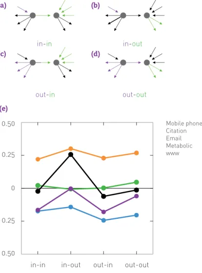
The degree correlation function (7.7) is defined for undirected net-works. To measure correlations in directed networks we must take into account that each node i is characterized by an incoming kin _and an outgoing kout _{degree [14]. We therefore define four degree} correla-tion funccorrela-tions, knnα,β(k), where α and β refer to the in and out indices (Figures 7.11 a-d). In Figure 7.11e we show knnα,β(k) for citation networks, in-dicating a lack of in-out correlations and the presence of assortativity for small k for the other three correlations (in-in, out-in, out-out).

DEGREE CORRELATIONS DEGREE CORRELATIONS IN REAL NETWORKS

i

i

(a)-(d) The four possible correlations charac-terizing a directed network. We show in purple and green the (α, β) indices that define the appropriate correla-tion funccorrela-tion [14]. For example, (a) describes the knn in,in(k) correlations be-tween the in-degrees of two nodes connected by a link.

(e) The kα, β

nn (k) correlation function for ci-tation networks, a directed network. For example knn in,in(k) is the average in-degree of the in-neighbors of nodes with in-degree kin. These functions show a clear assortative tendency for three of the four functions up to de-gree k ≃ 100. The empty symbols cap-ture the degree randomized kα, β

nn (k) for each degree correlation function (R-S randomization).

Figure 7.11

Correlations in Directed Network

10

2

10

1

10

0

10

0

10

1

10

2

10

3

10

4

10

3

in-in

in-out

out-in

out-out

in-in

in-out

out-in

out-out

a

c

d

b

k

_nn

(k

_β

)

k

_β α, β

10

2

10

1

10

0

10

0

10

1

10

2

10

3

10

4

10

3

in-in

in-out

out-in

out-out

in

-

in

in

-

out

out

-

in

out

-

out

k

_nn

(k

_β

)

k

_β α, β (a) (c) (e) (b) (d)

20 DEGREE CORRELATIONS

SECTION 7.6

To explore the impact of degree correlations on various network char-acteristics we must first understand the correlations characterizing the network models discussed thus far. It is equally important to develop algo-rithm that can generate networks with tunable correlations. As we show in this section, given the conflict between the scale-free property and degree correlations, this is not a trivial task.

DEGREE CORRELATIONS IN STATIC MODELS Erd_ős-Rényi Model

The random network model is neutral by definition. As it lacks hubs, it does not develop structural correlations either. Hence for the Erdő s-Rényi network knn(k) is given by (7.9), predicting μ = 0 for any ⟨k⟩ and N. Configuration Model

The configuration model (Figure 4.15) is also neutral, independent of the choice of the degree distribution pk. This is because the model allows for both multi-links and self-loops. Consequently, any conflicts caused by the hubs are resolved by the multiple links between them. If, however, we force the network to be simple, then the generated network will de-velop structural disassortativity (Figure 7.8).

Hidden Parameter Model

In the model ejk is proportional to the product of the randomly chosen hidden variables ηj and ηk (Figure 4.18). Consequently the network is tech-nically uncorrelated. However, if we do not allow multi-links, for scale-free networks we again observe structural disassortativity. Analytical calculations indicate that in this case [18]

knn(k) ~ k−1,

i.e. the degree correlation function follows (7.10) with μ = − 1.

Taken together, the static models explored so far generate either neu-tral networks, or networks characterized by structural disassortativity following (7.16).

GENERATING

CORRELATED NETWORKS

21

DEGREE CORRELATIONS GENERATING CORRELATED NETWORKS

DEGREE CORRELATIONS IN EVOLVING NETWORKS

To understand the emergence (or the absence) of degree correlations in growing networks, we start with the initial attractiveness model ( SEC-TION 6.5), which includes as a special case the Barabási-Albert model.

Initial Attractiveness Model

Consider a growing network in which preferential attachment follows

(6.23), i.e. Π(k) ∼ A + k, where A is the initial attractiveness. Depending on the value of A, we observe three distinct scaling regimes [15]:

(i) Disassortative Regime: γ < 3 If − m < A < 0 we have

Hence the resulting network is disassortative, knn(k) decaying follow-ing the power-law [15, 16]

(ii) Neutral Regime: γ = 3

If A = 0 the initial attractiveness model reduces to the Barabási-Al-bert model. In this case

Consequently knn(k) is independent of k, hence the network is neu-tral.

(iii) Weak Assortativity:γ > 3

If A > 0 the calculations predict

As k_nn(k) increases logarithmically with k, the resulting network dis-plays a weak assortative tendency, but does not follow (7.10).

In summary, (7.17) - (7.20) indicate that the initial attractiveness model generates rather complex degree correlations, from disassortativity to weak assortativity. Equation (7.19) also shows that the network gener-ated by the Barabási-Albert model is neutral. Finally, (7.17) predicts a power law k-dependence for knn(k), offering analytical support for the empirical scaling (7.10).

Bianconi-Barabási Model

With a uniform fitness distribution the Bianconi-Barabási model gen-erates a disassortative network [5] (Figure 7.12). The fact that the ran-domized version of the network is also disassortative indicates that the model's disassortativity is structural. Note, however, that the real knn(k)

The degree correlation function of the Bian-coni-Barabási model for N = 10,000, m = 3 and uniform fitness distribution (SECTION 6.2). As the green dotted line indicates, follwing (7.10)

indicates, the network is disassortative, con-sistent with μ ≃ -0.5. The orange symbols cor-respond to knn (k). As knn (k) also decreases, the bulk of the observed disassortativity is struc-tural. But the difference between knn(k) and knn (k) suggests that structural effects cannot fully account for the observed degree correlation.

R-S

R-S R-S

Figure 7.12

Correlations in the Bianconi-Barabási Model

(7.17) (7.18) (7.19) (7.20) knn(k)m (m+A) 1−A m 2m+A ς⎛⎝⎜2m2m+A⎞⎠⎟N − A 2m+A_kmA knn(k)∼k −_mA knn(k)m₂ln N. knn(k)≈(m+A)ln⎛_⎝⎜mk_+A⎞_⎠⎟.

>

10 10 10 Randomized (R-S)

~k

-0.5 10 10 0 1 2 3 4 ₁₀5 103 102 101 k_nn(k) k

22 DEGREE CORRELATIONS DISASSORTATIVE ASSORTATIVE · · · ··· · · · ··· (c) (d) (e) (f) k=3 kmax kmax k=3 k=2 k=2 k=1 k=3 k=2 k=1 k=1 k=3 k=2 k=1 ka≥kb≥kc≥kd DISASSORTATIVE ASSORTATIVE

STEP 1 LINK SELECTION

STEP 2 REWIRE (a) (b) 102 101 100 Assortative Neutral Disassortative 100 ₁₀1 ₁₀2 k_nn(k) k c b a d DISASSORTATIVE ASSORTATIVE

· · ·

···

· · ·

···

(c)

(d)

(e)

(f)

k=3 k_max k_max k=3 k=2 k=2 k=1 k=3 k=2 k=1 k=1 k=3 k=2 k=1 ka≥kb≥kc≥kd DISASSORTATIVE ASSORTATIVE

STEP 1 LINK SELECTION

STEP 2 REWIRE (a) (b) 102 101 100 Assortative Neutral Disassortative 100 101 ₁₀2

k

_nn

(k)

k

c b a d DISASSORTATIVE ASSORTATIVE · · · ··· · · · ··· (c) (d) (e) (f) k=3 kmax kmax k=3 k=2 k=2 k=1 k=3 k=2 k=1 k=1 k=3 k=2 k=1 ka≥kb≥kc≥kd DISASSORTATIVE ASSORTATIVE

STEP 1 LINK SELECTION

STEP 2 REWIRE (a) (b)₁₀2 101 100 Assortative Neutral Disassortative 100 ₁₀1 ₁₀2 knn(k) k c b a d DISASSORTATIVE ASSORTATIVE

· · ·

···

· · ·

···

(c)

(d)

(e)

(f)

k=3 k_max k_max k=3 k=2 k=2 k=1 k=3 k=2 k=1 k=1 k=3 k=2 k=1 ka≥kb≥kc≥kd DISASSORTATIVE ASSORTATIVE

STEP 1 LINK SELECTION

STEP 2 REWIRE (a) (b) 102 101 100 Assortative Neutral Disassortative 100 101 ₁₀2

k

_nn

(k)

k

c b a d

GENERATING CORRELATED NETWORKS

The algorithm generates networks with maximal degree correlations.

(a) The basic steps of the algorithm.

(b)knn(k) for networks generated by the al-gorithm for a scale-free network with N = 1,000, L = 2,500, γ = 3.0.

(c, d) A typical network configuration and the corresponding Aij matrix for the maximally assortative network generated by the algorithm, where the rows and col-umns of A_ij were ordered according to in-creasing node degrees k.

(e,f) Same as in (c,d) for a maximally disas-sortative network.

The Aij matrices (d) and (f) capture the in-ner regularity of networks with maximal correlations, consisting of blocks of nodes that connect to nodes with similar degree in (d) and of blocks of nodes that connect to nodes with rather different degrees in (f).

Xulvi-Brunet & Sokolov Algorithm

DISASSORTATIVE ASSORTATIVE

· · ·

···

· · ·

···

(c)

(d)

(e)

(f)

k=3 kmax kmax k=3 k=2 k=2 k=1 k=3 k=2 k=1 k=1 k=3 k=2 k=1 ka≥kb≥kc≥kd DISASSORTATIVE ASSORTATIVE

STEP 1 LINK SELECTION

STEP 2 REWIRE (a) (b) ₁₀₂ 101 100 Assortative Neutral Disassortative 100 101 ₁₀2

k

_nn

(k)

k

c

b

a

d

Figure 7.13 (a) (c) (e) (d) (f) (b) ASSORTATIVE DISASSORTATIVE

23

DEGREE CORRELATIONS GENERATING CORRELATED NETWORKS

and the randomized knn R-S (k) do not overlap, indicating that the disassor-tativity of the model is not fully explained by its scale-free nature. TUNING DEGREE CORRELATIONS

Several algorithms can generate networks with desired degree correla-tions [8, 17, 18]. Next we discuss a simplified version of the algorithm proposed by Xalvi-Brunet and Sokolov that aims to generate maximally correlated networks with a predefined degree sequence [19, 20, 21]. It consists of the following steps (Figure 7.13a):

• Step 1: Link Selection

Choose at random two links. Label the four nodes at the end of these two links with a, b, c, and d such that their degrees are ordered as

ka ≥ kb ≥ kc ≥ kd. • Step 2: Rewiring

Break the selected links and rewire them to form new pairs. Depend-ing on the desired degree correlations the rewirDepend-ing is done in two ways:

• Step 2A: Assortative

By pairing the two highest degree nodes (a with b) and the two lowest degree nodes (c with d), we connect nodes with compara-ble degrees, enhancing the network’s assortative nature.

• Step 2B: Disassortative

By pairing the highest and the lowest degree nodes (a with d and b with c), we connect nodes with different degrees, enhancing the network’s disassortative nature.

By iterating these steps we gradually enhance the network’s assortative (Step 2A) or disassortative (Step 2B) features. If we aim to generate a simple network (free of multi-links), after Step 2 we check whether the particular rewiring leads to multi-links. If it does, we reject it, returning to Step 1.

The correlations characterizing the networks generated by this algo-rithm converge to the maximal (assortative) or minimal (disassortative) value that we can reach for the given degree sequence (Figure 7.13b). The model has no difficulty creating disassortative correlations (Figures 7.13e,f). In the assortative limit simple networks display a mixed knn(k): assortative for small k and disassortative for high k (Figures 7.13b). This is a consequence of structural cutoffs: For scale-free networks the system is unable to sus-tain assortativity for high k. The observed behavior is reminiscent of the knn(k) function of citation networks (Figure 7.10j).

The version of the Xalvi-Brunet & Sokolov algorithm introduced in Fig-ure 7.13 generates maximally assortative or disassortative networks. We can tune the magnitude of the generated degree correlations if we use the algorithm discussed in Figure 7.14.

In summary, static models, like the configuration or hidden parameter model, are neutral if we allow multi-links, and develop structural disas-sortativity if we force them to generate simple networks. To generate net-works with tunable correlations, we can use for example the Xalve-Brunet & Sokolov algorithm. An important result of this section is (7.16) and (7.18), offering the analytical form of the degree correlation function for the hid-den paramenter model and for a growing network, in both case predicting a power-law k-dependence. These results offer analytical backing for the scaling hypothesis (7.10), indicating that both structural and dynamical ef-fects can result in a degree correlation function that follows a power law.

INTRODUCTION 24

25

DEGREE CORRELATIONS GENERATING CORRELATED NETWORKS

We can use the Xalvi-Brunet & Sokolov algo-rithm to tune the magnitude of degree cor-relations.

(a) We execute the deterministic rewiring step with probability p, and with probability 1 − p we randomly pair the a, b, c, d nodes with

each other. For p = 1 we are back to the

al-gorithm of Figure 7.13, generating maximal degree correlations; for p < 1 the induced

noise tunes the magnitude of the effect.

(b) Typical network configurations generated for p = 0.5.

(c) The knn(k) functions for various p values for

a network with N = 10,000, ⟨k⟩ = 1, and γ = 3.0.

Note that the correlation exponent μdepends on the fitting region, especially in the assor-tative case.

Figure 7.14

Tuning Degree Correlations

ASSORTATIVE DISASSORTATIVE

b

a

c

b

a

c-d

a-b

b-c

a-d

d

ka≥ kb≥ kc≥ kd DISASSORTATIVE

1 - p

p

RANDOMREWIRE ASSORTATIVE

STEP 1 LINK SELECTION STEP 2 REWIRE

c

ASSORTATIVE DISASSORTATIVE 102 102 101 101 100 p=0.2 p=0.4 p=0.6 p=0.8 p=1.0 p=1.0 p=0.2 µ=-0.064 p=0.4 µ=-0.080 p=0.6 µ=-0.085 p=0.8 µ=-0.095 k_nn(k) k 10 2 102 101 101 100 k_nn(k) k (a)

ASSORTATIVE

DISASSORTATIVE

b

a

c

b

a

c-d

a-b

b-c

a-d

d

ka ≥ kb ≥ kc≥ kd DISASSORTATIVE

1 - p

p

RANDOMREWIRE ASSORTATIVE

STEP 1

LINK SELECTION

STEP 2

REWIRE

c

ASSORTATIVE

DISASSORTATIVE

10

2

10

2

10

1

10

1

10

0 p=0.2 p=0.4 p=0.6 p=0.8 p=1.0 p=1.0 p=0.2 µ=-0.064 p=0.4 µ=-0.080 p=0.6 µ=-0.085 p=0.8 µ=-0.095

k

_nn

(k)

k

10

2

10

2

10

1

10

1

10

0

k

_nn

(k)

k

ASSORTATIVE

DISASSORTATIVE

b

a

c

b

a

c-d

a-b

b-c

a-d

d

ka≥ kb ≥ kc≥ kd DISASSORTATIVE

1 - p

p

RANDOMREWIRE ASSORTATIVE

STEP 1

LINK SELECTION

STEP 2

REWIRE

c

ASSORTATIVE

DISASSORTATIVE

10

2

10

2

10

1

10

1

10

0 p=0.2 p=0.4 p=0.6 p=0.8 p=1.0 p=1.0 p=0.2 µ=-0.064 p=0.4 µ=-0.080 p=0.6 µ=-0.085 p=0.8 µ=-0.095

k

_nn

(k)

k

10

2

10

2

10

1

10

1

10

0

k

_nn

(k)

k

(c)

_ASSORTATIVE

_{DISASSORTATIVE}

b

a

c

b

a

c-d

a-b

b-c

a-d

d

ka≥ kb ≥ kc≥ kd DISASSORTATIVE

1 - p

p

RANDOMREWIRE ASSORTATIVE

STEP 1

LINK SELECTION

STEP 2

REWIRE

c

ASSORTATIVE

DISASSORTATIVE

10

2

10

2

10

1

10

1

10

0 p=0.2 p=0.4 p=0.6 p=0.8 p=1.0 p=1.0 p=0.2 µ=-0.064 p=0.4 µ=-0.080 p=0.6 µ=-0.085 p=0.8 µ=-0.095

k

_nn

(k)

k

10

2

10

2

10

1

10

1

10

0

k

_nn

(k)

k

ASSORTATIVE

DISASSORTATIVE

b

a

c

b

a

c-d

a-b

b-c

a-d

d

ka≥ kb≥ kc≥ kd DISASSORTATIVE

1 - p

p

RANDOMREWIRE ASSORTATIVE

STEP 1

LINK SELECTION

STEP 2

REWIRE

c

ASSORTATIVE

DISASSORTATIVE

10

2

10

2

10

1

10

1

10

0 p=0.2 p=0.4 p=0.6 p=0.8 p=1.0 p=1.0 p=0.2 µ=-0.064 p=0.4 µ=-0.080 p=0.6 µ=-0.085 p=0.8 µ=-0.095

k

_nn

(k)

k

10

2

10

2

10

1

10

1

10

0

k

_nn

(k)

k

ASSORTATIVE ASSORTATIVE (b) DISASSORTATIVE DISASSORTATIVE

26 DEGREE CORRELATIONS

SECTION 7.7

As we have seen in Figure 7.10, most real networks are characterized by some degree correlations. Social networks are assortative; biological net-works display structural disassortativity. These correlations raise an im-portant question: Why do we care? In other words, do degree correlations alter the properties of a network? And which network properties do they influence? This section addresses these important questions.

An important property of a random network is the emergence of a phase transition at ⟨k⟩ = 1, marking the appearance of the giant compo-nent (SECTION 3.6). Figure 7.15 shows the relative size of the giant component for networks with different degree correlations, documenting several pat-terns [8, 19, 20]:

• Assortative Networks

For assortative networks the phase transition point moves to a lower

⟨k⟩, hence a giant component emerges for ⟨k⟩ < 1. The reason is that it is easier to start a giant component if the high-degree nodes seek out each other.

• Disassortative Networks

The phase transition is delayed in disassortative networks, as in these the hubs tend to connect to small degree nodes. Consequently, disas-sortative networks have difficulty forming a giant component. • Giant Component

For large ⟨k⟩ the giant component is smaller in assortative networks than in neutral or disassortative networks. Indeed, assortativity forc-es the hubs to link to each other, hence they fail to attract to the giant component the numerous small degree nodes.

These changes in the size and the structure of the giant component have implications to the spread of diseases [22, 23, 24], the topic of CHAPTER 10. Indeed, as we have seen in Figure 7.10, social networks tend to be assorta-tive. The high degree nodes therefore form a giant component that acts as

THE IMPACT OF DEGREE

CORRELATIONS

Relative size of the giant component for an Erdős-Rényi network of size N=10,000 (green curve), which is then rewired using the Xalvi-Brunet & Sokolov algorithm with p = 0.5 to induce degree correlations (Figure 7.14). The figure indicates that as we move from assor-tative to disassorassor-tative networks, the phase transition point is delayed and the size of the giant component increases for large ⟨k⟩. Each point represents an average over 10 indepen-dent runs.

Figure 7.15

Degree Correlations and the Phase Transition Point Assortative Neutral Disassortative 0.2 0 0.5 1 1.5 k S/N 2 2.5 3 0.6 0.8 1 0.4

27

DEGREE CORRELATIONS THE IMPACT OF DEGREE CORRELATIONS

a “reservoir” for the disease, sustaining an epidemic even when on average the network is not sufficiently dense for the virus to persist.

The altered giant component has implications for network robustness as well [25]. As we discuss in CHAPTER 8, the removal of a network's hubs fragments a network. In assortative networks hub removal makes less damage because the hubs form a core group, hence many of them are re-dundant. Hub removal is more damaging in disassortative networks, as in these the hubs connect to many small-degree nodes, which fall off the net-work once a hub is deleted.

Let us mention a few additional consequences of degree correlations: • Figure 7.16 shows the path-length distribution of a random network

re-wired to display different degree correlations. It indicates that in as-sortative networks the average path length is shorter than in neutral networks. The most dramatic difference is in the network diameter, dmax, which is significantly higher for assortative networks. Indeed, assortativity favors links between nodes with similar degree, result-ing in long chains of k = 2 nodes, enhancing d_max (Figure 7.13c).

• Degree correlations influence a system’s stability against stimuli and perturbations [26] as well as the synchronization of oscillators placed on a network [27, 28].

• Degree correlations have a fundamental impact on the vertex cover problem [29], a much-studied problem in graph theory that requires us to find the minimal set of nodes (cover) such that each link is con-nected to at least one node in the cover (BOX 7.4).

• Degree correlations impact our ability to control a network, altering the number of input signals one needs to achieve full control [30]. In summary, degree correlations are not only of academic interest, but they influence numerous network characteristics and have a discernable impact on many processes that take place on a network.

Distance distribution for a random network with size N = 10, 000 and ⟨k⟩ = 3. Correlations are induced using the Xalvi-Brunet & Sokolov algorithm with p = 0.5 (Figure 7.14). The plots show that as we move from disassortative to assortative networks, the average path length decreases, indicated by the gradual move of the peaks to the left. At the same time the di-ameter, d_max, grows. Each curve represents an average over 10 independent networks.

Figure 7.16

Degree Correlations and Path Lengths 0.05 0 5 10 _d 15 dmax = 24 dmax = 18 dmax = 21 pd 20 25 0.15 0.2 0.25 0.3 Assortative Neutral Disassortative 0.1

28

BOX 7.4

VERTEX COVER AND MUSEUM GUARDS

Imagine that you are the director of an open-air museum located in a large park. You wish to place guards on the crossroads to observe each path. Yet, to save cost you want to use as few guards as possible. How many guards do you need?

Let N be the number of crossroads and m < N is the number of guards you can afford to hire. While there are (m) ways of placing the m guards at N crossroads, most configurations leave some paths unsupervised [31].

The number of trials one needs to place the guards so that they cover all paths grows exponentially with N. Indeed, this is one of the six ba-sic NP-complete problems, called the vertex cover problem. The vertex cover of a network is a set of nodes such that each link is connected to at least one node of the set (Figure 7.17). NP-completeness means that there is no known algorithm which can identify a minimal vertex cover substantially faster than using as exhaustive search, i.e. check-ing each possible configuration individually. The number of nodes in the minimal a vertex cover depends on the network topology, being affected by the degree distribution and degree correlations [29].

DEGREE CORRELATIONS THE IMPACT OF DEGREE CORRELATIONS

Formally, a vertex cover of a network is a

set C of nodes such that each link of the

network connects to at least one node

in C. A minimum vertex cover is a vertex

cover of smallest possible size. The figure above shows examples of minimum ver-tex covers in two small networks, where the set C is shown in purple. We can check that if we turn any of the purple nodes into green nodes, at least one link will not connect to a purple node.

Figure 7.17

The Minimum Cover