DigitalCommons@USU
DigitalCommons@USU
All Graduate Theses and Dissertations Graduate Studies
5-2010
Random Forests Applied as a Soil Spatial Predictive Model in Arid
Random Forests Applied as a Soil Spatial Predictive Model in Arid
Utah
Utah
Alexander Knell Stum
Utah State University
Follow this and additional works at: https://digitalcommons.usu.edu/etd
Part of the Geographic Information Sciences Commons, and the Soil Science Commons
Recommended Citation Recommended Citation
Stum, Alexander Knell, "Random Forests Applied as a Soil Spatial Predictive Model in Arid Utah" (2010). All Graduate Theses and Dissertations. 736.
https://digitalcommons.usu.edu/etd/736
This Thesis is brought to you for free and open access by the Graduate Studies at DigitalCommons@USU. It has been accepted for inclusion in All Graduate Theses and Dissertations by an authorized administrator of DigitalCommons@USU. For more information, please contact [email protected].
RANDOM FORESTS APPLIED AS A SOIL SPATIAL PREDICTIVE MODEL IN ARID UTAH
by
Alexander Knell Stum
A thesis submitted in partial fulfillment of the requirements for the degree
of MASTER OF SCIENCE in Soil Science Approved: ________________________ ________________________
Dr. Janis L. Boettinger Dr. R. Douglas Ramsey
Major Professor Committee Member
________________________ ________________________
Dr. Michael White Dr. Byron R. Burnham
Committee Member Dean of Graduate Studies
UTAH STATE UNIVERSITY Logan, Utah
ABSTRACT
Random Forests Applied as a Soil Spatial Predictive Model in Arid Utah
by
Alexander Knell Stum, Master of Science Utah State University, 2010
Major Professor: Janis L. Boettinger Department: Plant, Soils, and Climate
Initial soil surveys are incomplete for large tracts of public land in the western USA. Digital soil mapping offers a quantitative approach as an alternative to traditional soil mapping. I sought to predict soil classes across an arid to semiarid watershed of western Utah by applying random forests (RF) and using environmental covariates derived from Landsat 7 Enhanced Thematic Mapper Plus (ETM+) and digital elevation models (DEM). Random forests are similar to classification and regression trees (CART). However, RF is doubly random. Many (e.g., 500) weak trees are grown (trained)
independently because each tree is trained with a new randomly selected bootstrap sample, and a random subset of variables is used to split each node. To train and validate the RF trees, 561 soil descriptions were made in the field. An additional 111 points were added by case-based reasoning using aerial photo interpretation. As RF makes
uncertainty can be derived. The overall out of the bag (OOB) error was lower without weighting of classes; weighting increased the overall OOB error and the resulting output did not reflect soil-landscape relationships observed in the field. The final RF model had an OOB error of 55.2% and predicted soils on landforms consistent with soil-landscape relationships. The OOB error for individual classes typically decreased with increasing class size. In addition to the final classification, I determined the second and third most likely classification, model confidence, and the hypothetical extent of individual classes. Pixels that had high possibility of belonging to multiple soil classes were aggregated using a minimum confidence value based on limiting soil features, which is an effective and objective method of determining membership in soil map unit associations and
complexes mapped at the 1:24,000 scale. Variables derived from both DEM and Landsat
7 ETM+ sources were important for predicting soil classes based on Gini and standard measures of variable importance and OOB errors from groves grown with exclusively DEM- or Landsat-derived data. Random forests was a powerful predictor of soil classes and produced outputs that facilitated further understanding of soil-landscape
relationships.
ACKNOWLEDGMENTS
I want to thank the Utah Agricultural Experiment Station and the Bureau of Land Management (BLM) of Utah for funding this research. And special thanks to Lisa Bryant with the BLM for her direct support in the field and her desire to apply this kind of research in the field.
Kent Sutcliffe and Tom Simper with the Natural Resources Conservation Service (NRCS) gave invaluable technical assistance, teaching me all the local plants, including me on field reviews, sharing knowledge of soil-landscape relationships, and much more.
My days in the field would have been at times unbearable without the company of my friends and undergraduate assistants Morgan Koenig and Colby Brungard. There is no way I could have canvassed so much area and remained so focused without them. I especially want to thank Colby whose desire to learn inspired me further.
I simply marvel at Janis’s aptitude to learn and deeply understand what each of her graduate students have done. My research has been no exception. I have learned so much from her in and out of the academic setting. Thank you for your continual support these many years.
This task could not have been completed without the gentle (sometimes urgent) persuasions of my mother (Rebecca Stum) and also my wife, Marci. Marci has sacrificed and given more than anyone else to get me here. I love you and thank you.
CONTENTS
Page
ABSTRACT ... ii
ACKNOWLEDGMENTS ... iv
LIST OF TABLES ... vii
LIST OF FIGURES ... ix
INTRODUCTION ... 1
Soil Formation – A Theoretical Framework ... 2
Digital Soil Mapping – A Spatial Framework ... 2
Objective ... 4
LITERATURE REVIEW ... 6
Environmental Covariates ... 6
Soil Properties (s) & Parent Material (p) ... 7
Climate (c) ... 8
Organisms (o) ... 9
Relief (r) ... 10
Time (a) ... 10
Spatial Position (n) ... 11
Soil Spatial Prediction Functions ... 12
STUDY AREA DESCRIPTION ... 16
Climate (c) ... 16
Organisms (o) – Vegetation ... 19
Parent Material (p) – Geology ... 21
Proterozoic to Early Cambrian ... 21
Paleozoic ... 23
Mesozoic ... 23
Cenozoic ... 24
Tertiary ... 24
Soil (s) ... 31
METHODOLOGY ... 33
Digital Data ... 33
Landsat-Derived Data ... 33
Digital Elevation Model-Derived Data ... 40
Digital Data Exploration and Transformation... 44
Customized Data Layers ... 45
Field Work ... 53
Predicting Soil Classes Using Random Forests ... 54
Soil Classes ... 54
Sampling of Digital Data ... 58
Random Forests Model ... 61
Variable Importance ... 63
Components and Map Units ... 63
RESULTS AND DISCUSSION ... 67
Groves 1A and 1B ... 67 Groves 2A and 2B ... 70 Grove 2B ... 75 Variable Importance ... 77 OOB ... 80 Model Confidence ... 83 Individual Components ... 86 Map Units ... 98 CONCLUSION ... 100 REFERENCES ... 103 APPENDICES ... 110 Appendix A: R Code ... 111
Appendix B: Prediction of Soil Attributes ... 116
Appendix C: Spectral and Topographic Characteristics ... 121
Appendix D: Natural Break - Overlay ... 127
LIST OF TABLES
Table Page
1 Orders of soil mapping ………... 4
2 Landsat 7 ETM+ spectral and spatial resolution of each band ……….. 9
3 Geologic chronology ……… 22
4 Environmental covariates represented by digital data ………. 34
5 The bounding coordinates of each independent variable source and the study area ………. 35
6 The general taxonomic class and soil series name of each predicted class ……. 59
7 The four groves selected for comparison of outputs ……… 63
8 Summary of the OOB error matrix for Groves 1A and 1B ……….. 68
9 Summary of the OOB error matrix for Groves 2A and 2B ……….. 71
10 A comparison of OOB error rates for 66 groves grown using the same parameters as Grove 2B ……….. 76
11 Variable importance from Random Forests Grove 2B ………..……... 79
12 The error matrix summarizes the OOB results by class ……….. 81
13 The Random Forests result from Grove 2B for an individual pixel in the San Francisco Mountains ………...…….. 84
14 A summary of Grove 2B ……….. 90
15 The prediction summary of diagnostic features ……….…… 118
16 The percentage of each soil class stratified into a categorical variable class for the 671 sample points and all pixels in the study area ………. 123
17 The average value of the continuous environmental covariates for the sample data ………. 124
18 The average value of each continuous environmental covariate of each pixel according to their predicted class……… 125
19 The Mean and Standard Deviation of each
continuous environmental covariate for all pixels in the study area ………….. 126
20 The distribution of all OOB votes summarized by class ………136
LIST OF FIGURES
Figure Page
1 Study area location in the state of Utah ………... 17
2 The Big Wash study area shown in a Landsat 7 scene false color (bands 5, 7, 1) ………. ………... 18
3 Aerial photograph of the SW slope of the Beaver Lake Mountains ………….... 28
4 Photograph looking northwest towards the San Francisco Mountains ……….... 32
5 Landsat 7 ETM+ imagery ……… 36
6 Landsat 7 ETM+ imagery ……….... 37
7 Normalized difference ratios of Landsat 7 ETM+ ………... 38
8 Normalized difference ratios of Landsat 7 ETM+ ………... 39
9 Normalized difference ratio of Landsat 7 ETM+ ……….... 40
10 DEM-derived data ……….... 42
11 DEM-derived data ……….... 43
12 Illustration of the transformation of aspect in degrees to continuous variable of north-south ranging from -π to π ………..……... 44
13 The Lake Bonneville shoreline prediction ………... 47
14 Feature space plot of Landsat 7 ETM+ (non-standardized) bands 3 and 4 ……….…….. 49
15 Climogeomorphic breaks ………... 50
16 The elevation range relative to aspect for each SMR ……….……... 51
17 Training data set for the random forests models ……….. 60
18 Conceptual example of an Imagine .ckb model ………... 66
20 The results of Groves 2A (A) and 2B (B) ……… 72
21 A comparison of Groves 1B (A) and 2B (B) ………... 74
22 The OOB error of groves grown with random subsets of the whole dataset …... 82
23 Model prediction outputs of Grove 2B. ………... 87
24 Model confidence outputs of Grove 2B ………... 88
25 The hypothetical extents of classes 1 (A), 2 (B), 3 (C), and 4 (D) ……….. 91
26 The hypothetical extents of classes 5 (A), 6 (B), 7 (C), and 8 (D)…………... 92
27 The hypothetical extents of classes 9 (A), 10 (B), 11 (C), and 12 (D) ………… 93
28 The hypothetical extents of classes 13 (A), 14 (B), 15 (C), and 16 (D) ……... 94
29 The hypothetical extents of classes 17 (A), 18 (B), 19 (C), and 20 (D) …..…… 95
30 The hypothetical extents of classes 21 (A), 22 (B), 23 (C), and 24 (D) ……….. 96
31 The hypothetical extents of Dixie (green) and Garbo (red) ………... 97
32 The results of the soil class combinations ……… 99
33 Prediction of diagnostic features ……… 119
34 Prediction of the three most common particle size family classes (texture classes) ………. 120
35 The area of interest selected for the natural breaks overlay process ………….. 130
36 Aerial photography ……… 131
37 Results of the natural breaks exercise ……… 132
38 Comparison of the Random Forest classification (A) to Random Forests laid over the unsupervised classification (B) ……… 133
INTRODUCTION
Knowledge of soil systems is necessary to understand our world's natural systems, geomorphology, hydrology, ecology, and climatology (Lookingbill and Urban, 2004). The incorporation of topographic and remotely sensed (RS) data into the study of soil systems has increased our ability to predict the spatial distribution of soils across the landscape (McBratney et al., 2003; Scull et al. 2003).
Typically, soils are represented on a thematic map made up of polygons
representing individual map units (Soil Survey Division Staff, 1993; Scull et al., 2003; USDA-NRCS, 2009). Each map unit represents the generalized distribution of soils in the landscape as an association, complex, consociation, or as undifferentiated (Moran and Bui, 2002). Soils or landscape features (e.g., rock outcrop) that are known to occur within a map unit are referred to as components. Components in an association can be delineated at the scale of mapping, whereas components of a complex cannot be delineated at the scale of mapping (Soil Survey Division Staff, 1993).
Traditional soil maps illustrate conceptual models of soil distribution on the landscape. When a soil scientist draws a line on the map he/she is predicting that certain soils are likely to be found within the delineated polygon. The parameters of this
conceptual model are complicated, and are related to the individual experience or tacit knowledge of the soil scientist, and are, therefore, subjective (Hudson, 1992).
Traditional soil survey methods, while thoroughly reviewed, are not assessed for accuracy. Many soil predictive models also produce uncertainty maps which can focus future field activities and give the user further information about the map. Ongoing
research in digital soil mapping has demonstrated that reasonably accurate soil maps can be produced using quantitative predictive models. Digital soil mapping may also expedite soil survey (Lagacherie and Holmes, 1997; Dobos et al., 2000; Zhu, 2000; Moran and Bui, 2002; McBratney et al., 2003; Scull et al., 2003; Cole, 2004; Shi et al., 2004; Henderson et al., 2005; Saunders, 2005; Scull et al., 2005; Cole and Boettinger, 2007; Saunders and Boettinger, 2007; Brungard, 2009).
Soil Formation – A Theoretical Framework
Hans Jenny (1941) presented an elegant function to explain the current state of a soil: S = f(c, o, r, p, t). Simply said, soil (S) is a function of five environmental factors: climate (c), organisms (o), relief (r), parent material (p), and time (t). While this function has proven difficult, if not impossible, to solve, it has set forth a theoretical framework whereby soil formation can be studied. To simplify the function and better understand soil formation, studies have focused on identifying transitions in soil properties along sequences of soils related to one environmental factor; such as climate (climosequences), time (chronosequences), relief (toposequences), etc. (Jenny, 1980; Birkeland, 1999).
Digital Soil Mapping – A Spatial Framework
Spatial data analysis seeks to elucidate some pattern or process that occurs in space, perhaps allowing us to make predictions where no observations have been made (Bailey and Gatrell, 1995). Based on Jenny’s soil forming factors (1941), McBratney et al. (2003) proposed an empirical formulation to quantitatively find correlations between spatially explicit data and the soil. They considered seven factors, or environmental
covariates, in their model, referred to as "scorpan." The five soil forming factors from Jenny (1941) are still present as covariates: ‘c’ climate; ‘o’ organisms, vegetation, fauna, and/or human activity; ‘r’ topography and landscape attributes; ‘p’ parent material, lithology; and ‘a’ time or age.
Two additional scorpan covariates are specifically directed towards spatial predictive models: ‘s’ soil or soil properties, and ‘n’ space, spatial position, or relative position. There are two general forms of the scorpan model (McBratney et al., 2003):
) , , , , , , ( ) , , , , , , (s c o r p a n or S f s c o r p a n f Sc = a =
where Sc is soil class and Sa is a soil attribute or property.
McBratney et al. (2002) demonstrated that some soil properties (e.g., saturated hydraulic conductivity) may be predicted from other soil properties (e.g. sand content) using quantitative functions, known as pedotransfer functions. Where a sufficient number of soil property observations are available, pedotransfer functions can be incorporated into spatial models to predict soil class or other soil attributes. Also, soil maps representing soil classes can help predict soil attributes. The general form of a soil spatial prediction function is ) ( ) , , , (x y z t f Q S =
where S is a soil located at coordinates x,y,z, for a period of time, t, and is a function of predictor variable(s) Q.
The values of predictor variables (independent variables) must be known at the points where the soil class or attributes are to be predicted.
Objective
The Bureau of Land Management (BLM) administers 258 million surface acres, mostly in the western United States (BLM, 2006). The BLM must make appropriate management decisions related to grazing allotments, recreational activities, fire restoration, mine reclamation, chaining, hydrologic studies, wildlife monitoring and much more. The BLM land managers need to know the spatial distribution of soils to support these management decisions.
For rangeland planning, the BLM normally needs third order soil survey maps at the 1:24,000 scale. Large tracts of BLM land have no soil data, or only have fourth order or fifth order soil maps which are completed at a very coarse spatial resolution and present insufficient detail for many land management activities (Table 1).
Table 1. Orders of soil mapping (Soil Survey Division Staff, 1993).
Mapping level Minimum-size
delineation [ha]
Appropriate map scale
1st Order – experimental plots, building sites 1 or less 1:15,840 or larger
2nd Order – agriculture/urban planning 0.6 to 4 1:12,000 to 1:31,680
3rd Order – range planning 1.6 to 16 1:20,000 to 1:63,360
4th Order – general soil information 16 to 252 1:63,360 to 1:250,000
5th Order – regional planning 252 to 4,000 1:250,000 to
The Natural Resources Conservation Service (NRCS) recently completed the soil mapping of privately owned lands in central Beaver County, Utah. The BLM manages 440,648 ha (1.14 million ac) of Beaver County, or 68.8% of the county’s area. Because of the high cost of traditional methods of soil mapping and the remoteness of much of the county, the BLM has been interested in facilitating the investigation of alternative soil mapping techniques. A 47,000-ha watershed northwest of Milford, Utah, was selected as a trial area to implement soil spatial predictive models to create a soil map. The objective of this study was to apply a soil spatial predictive model to create a soil map at the 1:24,000 scale with topographic and remotely sensed data as environmental covariates (soil-forming factors). I hypothesized that these spatially explicit data layers can be successfully incorporated into quantitative models (i.e. random forests) to predict soil types across the landscape and generate estimates of prediction uncertainty.
LITERATURE REVIEW
The following is a review of pertinent literature of scorpan environmental covariates and of spatial prediction functions and models.
Environmental Covariates
Most environmental covariates can be represented by remotely sensed spectral data or derivatives from digital elevation models. Satellite imagery and aerial
photography are remotely measured properties of the land surface itself, be it soil, water, geology, human infrastructure or various combinations of these. Electromagnetic (EM) radiation is reflected, absorbed, or emitted as a function of the physical and chemical properties of that surface (Goetz, 1989; Rees, 2001).
The topographic surface (x, y, z) can be represented in several formats, such as an isarithmic map (contour map), triangular irregular network (TIN), raster digital elevation model (DEM), and others (DeMers, 2000). The raster digital elevation model is the representation of a point data set as a raster surface. Each grid cell value is the predicted or interpolated elevation at the center or corner of the cell. Digital elevation models are the more commonly used in geographic information systems (GIS) environments because primary derivations, such as slope and aspect, can be easily calculated (Chaplot et al., 2006). Very useful secondary derivations, such as compound topographic index (CTI), specific catchment area, and stream networks can also be derived.
Soil Properties (s) & Parent Material (p)
Soil is a combination of inorganic solids, organic matter, gases, and soil water constituents. Each one of these influences the way in which electromagnetic radiation interacts with the soil surface. Teasing out specific soil properties from this surface signal can be difficult.
Gomez et al. (2008) modeled soil organic carbon by multivariate regression of Hyperion hyperspectral satellite imagery (242 bands in the visible and near infrared, 400-2500 nm). Anderson and Croft (2009) reviewed literature related to soil surface
roughness and soil moisture studies. They found promising applications of optical remote sensing to measure albedo and bidirectional reflection with regard to soil surface
roughness and physical structure. They also explored active microwave systems (e.g. ALOS, RADARSAT-2, and Terra SAR-X), which take advantage of the difference in dielectric constants between water and soil to determine soil surface moisture.
The largest constituent of the soils in this study area is the inorganic solids, which are primary and secondary minerals derived from the weathering of parent material (local geology) (Birkeland, 1999). These minerals may impart a unique spectral signature that can be used to identify the mineralogy of the soil surface (Goetz, 1989; Irons et al., 1989; McBratney et al., 2003). This information can be related to other soil attributes or classes.
El Rakaiby et al. (1994) measured in situ reflectance of geology members on the
Sinai Peninsula. The spectral signatures gathered in the field with handheld radiometers were analyzed and used to evaluate Landsat 7 ETM+ satellite imagery taken over the region. They determined that Landsat 7 ETM+ band ratios were effective in
the influence of shadows, as absolute brightness values of the satellite image are not being used but rather the relative brightness of one band compared to another (Goetz, 1989; Jensen, 2005).
Bodily (2005) used the normalized difference ratio of Landsat 7 ETM+ bands 5 and 2 to identify limestone outcroppings (Table 2). His findings were consistent with radiometric lab measurements of the spectral profile of limestone and dolomite, where limestone and dolomite have greater reflectance in band 5 relative to band 2 while andesite and other igneous materials have greater reflectance in band 2 relative to band 5 (NASA, 2008). Cole (2004) and Saunders (2005) incorporated simple Landsat band ratios (3/2, 3/7, and 5/7) with DEM-derived data to predict soil types with knowledge-based and decision tree classifications, respectively.
Nield et al. (2007) successfully used normalized difference band ratios with Landsat 7 ETM+ bands 5 and 7 and bands 5 and 4 to identify gypsic and natric soil areas, respectively, in an arid area of central Utah. Bands 5 and 7 appeared to be correlated with the occurrence of near-surface secondary gypsum, whereas bands 5 and 4 were most likely correlated with the co-occurrence of Fe-bearing desert varnish on surface rocks fragments near natric soil area training sites.
Climate (c)
Data layers that explicitly represent climatic variables at an appropriate scale (1:24000) are usually not readily available. For example, PRISM data has a spatial
resolution of approximately 4km (USDA-NRCS, 2000), which is too coarse for many 3rd
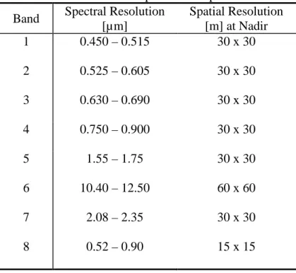
Table 2. Landsat 7 ETM+ spectral and spatial resolution of each band (Jensen, 2005).
Band Spectral Resolution
[µm] Spatial Resolution [m] at Nadir 1 0.450 – 0.515 30 x 30 2 0.525 – 0.605 30 x 30 3 0.630 – 0.690 30 x 30 4 0.750 – 0.900 30 x 30 5 1.55 – 1.75 30 x 30 6 10.40 – 12.50 60 x 60 7 2.08 – 2.35 30 x 30 8 0.52 – 0.90 15 x 15 Organisms (o)
Vegetation cover affects the absorbance and reflectance response of the land surface, and thus can be quantified using satellite imagery. Chlorophyll and other
pigments of plants absorb light in the visible spectrum (0.35-0.70 μm) for photosynthesis
(Jensen, 2005). This absorption feature is most pronounced around the blue (0.45-0.52
μm) and red (0.63-0.69 μm) portions of the visible spectrum. The spongy mesophyll layer
of the leaf transmits or reflects 90-95% of radiant energy from 0.7 to 1.2 μm in the near
infrared (NIR) portion of the spectrum. Therefore, the simple ratio of the measured
reflectance (ρ) of NIR to Red is greatest in areas of leafy vegetation. Normalized
difference vegetation index (NDVI) has most commonly been used to represent
vegetation in digital soil mapping (McBratney et al., 2003): NDVI
d NIR d NIR = + − Re Re ρ ρ ρ ρ
Relief (r)
Topography is the most commonly used soil factor in soil genesis studies related to soil catena (Birkeland, 1999; McBratney et al., 2003). Often, topography is the soil forming factor that expresses the most variation at the field scale and, therefore, must be addressed. Soil depth and soil production vary with slope and curvature (Heimsath et al., 1997). Aspect is an important control of soil microclimate and vegetation (Jenny, 1980). Gessler et al. (2000) demonstrated that compound topographic index (CTI), also referred to as the steady-state wetness index, is related to soil properties, such as A horizon
thickness:
β tan ln As
CTI =
where As is the specific catchment area (area [m2] per unit width [m]) and β is the slope
angle.
Time (a)
Time is the most difficult soil-forming factor to represent explicitly (McBratney et al., 2003; Noller, 2010) and at best only relative time can be assumed without
performing complicated and expensive dating procedures, e.g. luminescence, cosmogenic isotope dating, etc. Also, ages from these procedures would need to be interpolated or used to assume the age of entire surfaces. Specific geomorphic surfaces and positions may approximate relative age (Noller, 2010). Scull et al. (2005) represented time implicitly with Landsat imagery which can detect desert varnish.
Spatial Position (n)
Considering a pixel value in the context with its neighbors, or its spatial context, can enhance classification (Moran and Bui, 2002). Humans observe patterns, tonal differences, edges, etc. simultaneously. Generally, computer software can only consider each pixel individually and often cannot see the forest for the trees and/or the space between the trees. To add spatial relationships to the data set, various texture
transformations can be performed. A simple first-order statistical example is the use of a low pass filter. A pixel is assigned the average value of the neighboring pixel values. Variance and entropy are other first-order statistics in the spatial domain (Jensen, 2005). Similarly, Saunders (2005) buffered individual sample points to capture the range of characteristics within a map unit.
Relative position can be related to specific soil forming factors, such as proximity to a steep mountain slope or categorical distinctions. When strongly contrasting
pedogeomorphic or geologic regimes exist, McBratney et al. (2003) suggested that stratifying the study area into smaller physiographic regions may simplify the modeling process. Similar to a climosequence, where all factors are said to be constant except climate, stratification isolates regions where one or more factors are generally the same or similar. This allows the modeler to focus on the specific relationships between the soil and the environmental factors within each physiographic region (Di Paolo and Hall, 1983; Birkeland, 1999). Zhu (2000) stratified his study area by geology type before modeling the distribution of soil series using artificial neural networks. Scull et al. (2005) stratified their study area into two distinctive physiographic regions, basin and mountain
regions, improving the overall accuracy of their prediction with decision tree analysis (DTA).
Soil Spatial Prediction Functions
Initially, geographic information system (GIS) technologies for soil mapping focused on stratifying the area or creating topographic data layers derived from digital elevation models (e.g., slope and aspect), which assisted the soil scientist in line
placement on soil maps (Di Paolo and Hall, 1983; Amen and Foster, 1987). Since then, several workers have applied statistical models to predict both soil types and properties across the landscape (McBratney et al., 2003). Much of the current research in soil predictive models revolves around the method(s) by which the data are analyzed and the uncertainty of resulting predictions. Faster computers and more efficient software continually allow us to explore new techniques of data analysis.
Both McBratney et al. (2003) and Scull et al. (2003) extensively reviewed digital (predictive) soil mapping studies. Scull et al. (2003) generalized predictive soil mapping approaches into four categories: geostatistical methods (e.g., kriging), statistical methods (e.g., generalized linear models), decision tree analysis (e.g., classification and regression tree analysis), and expert systems (e.g., SoLIM [Shi et al., 2004]). Generally,
geostatistical and statistical methods are used in predicting soil attributes (Sa), where the
predicted outputs are continuous values (Scull et al., 2003). Logistic regression has been used to predict the presence or absence of soil features, such as an E horizon, and fuzzy logic has been used to predict soil classes (Odeh et al., 1992; Gessler et al., 1995).
Decision tree analysis and expert systems have usually been used to predict discrete soil
classes (Sc).
The pedogenic understanding raster-based classification (PURC) method was developed by Cole (2004), where conceptual models of the soil-landscape relationships were explicitly defined. Spatially explicit topographic and remotely sensed data
represented the soil forming factors. Initially, Cole produced unsupervised and supervised classifications of the individual data layers to identify patterns within the data. The
exploration and analysis of these data layers also guided future sampling, by allowing a soil scientist to observe which of these patterns may be meaningful. Rules for classifying data to represent conceptual models were created to predict soil distribution on the landscape.
The Soil-Land Inference Model (SoLIM) also incorporates expert knowledge from soil scientists (Zhu, 2000; Shi et al., 2004). Originally, Shi et al. (2004) had the soil scientist explicitly define the rules. But, they found that this approach can be complicated as it is difficult to explicitly make quantitative rules from tacit knowledge. Another complication arises from the assumption of independence between variables. This interplay between soil forming factors complicates the process of defining rules for each individual variable. To overcome this, Shi et al. (2004) took a case-based reasoning (CBR) approach. Similar to supervised classification, the soil scientist selects points and/or polygons within the GIS as training sites.
The significant difference between expert systems and decision trees is who makes the rules, the user or the data. Decision trees are data driven, where the data set (sample data) is divided with the objective of separating the data set into pure or
homogenous classes. At each node, an independent variable that most cleanly divides the data set is chosen. Recursively, splits are made with the objective of creating
homogenous groups. To mitigate over-fitting, trees are pruned, where branches are cut back to a higher node. After the tree is grown using training data, unknowns are thrown down the tree, and the class for that point is determined.
Moran and Bui (2002) used decision trees as a manner of machine learning or data mining. They input spatial data for multiple environmental variables to see if the computer could derive a set of rules to mimic or re-create the soil map of a previously mapped area. They were able to remap the area with 70% agreement with the original mapping of the soil scientists.
Moran and Bui (2002) also employed boosting and area-weighting, which
increased the accuracy and qualitative look of their prediction. Area-weighting samples in proportion to the spatial extent of the class, which can only work when the extent of the class is previously known. Boosting is a technique that reduces bias. Initially, a single tree is grown with all cases receiving equal weight. A new tree is grown where
misclassified cases are given more weight relative to correctly classified cases. This process is repeated a user-specified number of times. Each pixel is assigned to a class based on the modal result or “majority of votes” from the trees (Moran and Bui, 2002).
If the computer can capture the same soil patterns on the map, i.e. the conceptual model developed by the soil scientist, then the tree (the set of rules) could potentially predict the soils in unmapped areas. Scull et al. (2005) was able to take the next step with decision trees, extracting randomly sampled points from an existing soil survey, to train the trees and then extrapolate into areas that were not previously mapped.
Saunders (2005) was able to model soil map units as part of a third order soil survey in Wyoming in a previously unmapped area using classification tree analysis. The sample points were observations made in the field. To capture the range of environmental variables within a map unit, a buffer was set up around each point to sample the data layers (independent variables), reducing prediction error.
Developed by Breiman and Cutler (2009), random forests (RF) is an ensemble of classification and regression trees (CART). Random forests is said to be as accurate as or better than adaptive boosting, yet computationally faster (Breiman, 2001; Gislason et al., 2006). Instead of growing just one tree, many (hundreds to thousands) unpruned,
independent trees are grown. This ensemble of trees is referred to as a grove. Each tree is trained from an independent and random bootstrap sample, where a random subset of the sample is used to grow (train) the tree and the remaining points are left ("out of bag
sample") to test or validate the tree. Also, at each split, a random subset of predictor
variables is chosen (e.g., if there were 100 predictor variables, a subset of ten could be selected at random). From this random subset the strongest variable is selected to split the data. Because of the random bootstrap sample and the random subset of predictive
variables at each node, random forests is said to be doubly random. Unlike boosting, each tree is grown independent of each other to the maximum depth (no pruning). Like
boosting, the modal result of the entire grove determines the class membership. By making many weak, independent trees, random forests discern patterns in the data that otherwise may be overlooked when few strong trees are grown.
STUDY AREA DESCRIPTION
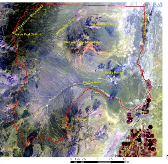
The study area is in the Basin and Range physiographic province, northwest of Milford in Beaver County, Utah (Figure 1).
The study area encompasses The Big Wash watershed and adjoining areas south of the Beaver-Millard County line, east of the crest of the San Francisco Mountains and west of the Beaver River bed (Beaver Bottoms), covering ~47,000 ha (~117,000 ac) (Figure 2). Each of the following sections addresses the five soil-forming factors of climate, organisms, parent material (geology), relief, and time within the study area.
Climate (c)
Situated between the Sevier and Escalante Deserts, the study area has an arid continental climate, with warm summers and cold winters. Precipitation estimates, from PRISM (Parameter-elevation Regressions on Independent Slopes Model) developed by Oregon State University, range from 20 cm (8 in.) at the Beaver Bottoms to 41 cm (16 in.) atop the San Francisco Mountains (see Figure 2) (USDA-NRCS, 2000). Milford has the nearest climate station, located at the airport with an elevation of 1533 m (5030 ft). National Climate Data Center (NCDC) 1961-1990 normal for Milford are 25.0 cm (9.84 in.) of annual precipitation, mean annual temperature of 9.3°C (48.8° F), mean summer temperature of 21.4° C (70.5° F) and -1.7° C (29.0° F) mean winter temperature (WRCC, 2005). The wettest months are March and April, when storms from the Pacific Ocean bring widespread rain and snow events. The driest time of the year is June into the beginning of July. Monsoonal moisture enters into the area in late July into September.
Precipitation during the summer is often associated with intense, convective thunderstorms which are often isolated.
The soil moisture regime across most of the area is aridic bordering on xeric (xeric aridic); meaning the soil is dry 50 to 75 percent of the time when the soil temperature is above 5ºC (Soil Survey Staff, 2003). In Utah, areas that are xeric aridic generally receive 8-12 inches of precipitation (Kent Sutcliffe, USDA-NRCS Utah, personal communication, 2005). The soil moisture regime of the Beaver Bottoms is typic aridic (dry >75 percent of the time when the soil temperature is above 5ºC). Much of the San Francisco Mountains have a xeric soil moisture regime (dry for 45 or more
consecutive days in the four months following the summer solstice and moist for 45 or more consecutive days in the four months following the winter solstice). The soil
temperature regime is mesic (mean annual soil temperature of 8-15ºC with ≥6ºC
difference between mean summer and mean winter soil temperatures) across the whole area, except for the top of the San Francisco Mountains where it is frigid (mean annual
soil temperature <8ºC with ≥6ºC difference between mean summer and mean winter soil
temperatures).
Organisms (o) – Vegetation
Vegetation in the Great Basin can be an important indicator of soil and climate characteristics. The vegetation in the study area has been grouped into four broad categories of commonly geographically associated species. Scientific names are from Winward (2004) or the Range Plants of Utah web page (USU Extension, 2009). The first group is a salt-desert community, generally found in the valley bottoms and playas where
soils are often saline, finer textured, and more alkaline (pH >8.5) in the rooting zone. The
plants are shadscale (Atriplex confertifolia), black greasewood (Sarcobatus
vermiculatus), four-wing saltbush (Atriplex canescens), budsage (Artemisia spinescens),
winterfat (Krascheninnikovia lanata), and squirrel tail (Elymus elymoides).
The second group is a sagebrush scrubland, which is the most prevalent
vegetation type in the study area. The plants include black sage (Artemisia nova),
Wyoming big sage (Artemisia tridentata ssp. wyomingensis), basin big sage (Artemisia
tridentata ssp. tridentata), spiny hopsage (Grayia spinosa), pygmy sage (Artemisia pygmaea), winterfat (Krascheninnikovia lanata), squirrel tail (Elymus elymoides),
needle-and-thread (Hesperostipa comata), indian rice grass (Achnatherum hymenoides), galleta
(Pleuraphis jamesii), scarlet globemallow (Sphaeralcea coccinea), cliffrose (Purshia stansburiana), rubber rabbitbrush (Chrysothamnus nauseosus), Douglas rabbitbrush (Chrysothamnus viscidiflorus), broom snakeweed (Gutierrezia sarothrae), ephedra (Ephedra viridis), and various species of Penstemon, Phlox, and Eriogonum.
The higher elevation terrain that surrounds the area is covered by open woodland
of Utah juniper (Juniperus osteosperma) and singleleaf pinyon (Pinus monophylla). The
understory vegetation is black sage (Artemisia nova), Wyoming big sage (Artemisia
tridentata ssp. wyomingensis), antelope bitterbrush (Purshia tridentata), bluebunch
wheatgrass (Agropyron spicatum), lupine (Lupinus sp.), Indian rice grass (Achnatherum
hymenoides), and needle-and-thread (Hesperostipa comata).
The higher elevations of the San Francisco Mountains are predominantly covered
by woodland composed of singleleaf pinyon (Pinus monophylla), Rocky Mountain
ponderosa pine (Pinus ponderosa), curlleaf mountain mahogany (Cercocarpus
ledifolius), limber pine (Pinus flexilis), lupine (Lupinus sp.), aspen (Populus tremuloides),
and white fir (Albies concolor).
Parent Material (p) – Geology
The soils in the study area have formed in parent materials derived from three distinct lithologies: metamorphic rocks from the Proterozoic, sedimentary rocks from the Paleozoic and early Mesozoic, and igneous rocks from the Tertiary and early Quaternary (Table 3).
Proterozoic to Early Cambrian
The oldest rocks exposed in the area make up the summit crests of the San
Francisco Mountains to the west and the very northern end of the Beaver Lake Mountains (East, 1966; Woodward, 1973; Hintze et al., 1984). These rocks represent six concordant units, from Proterozoic to early Cambrian, formed from initial deposits of the Cordilleran miogeosyncline: Cambrian Prospect Mountain Quartzite, Pre-Cambrian Mutual
Quartzite, Pre-Cambrian Inkon Slate, Proterozoic Caddy Canyon Quartzite, undivided Proterozoic Papoose Creek Argillite and Proterozoic Blackrock Canyon Limestone, and the upper member of Proterozoic Pocatello Quartzite (Woodward, 1973). While the map by Hintze et al. (1984) indicates that Frisco Peak is composed of Mutual Quartzite, a purple conglomerate quartzite, my observations indicate it is more likely the light pink to tan quartzite, Prospect Mountain Quartzite.
Table 3. Geologic chronology (U.S. Geological Survey Geologic Names Committee, 2007).
Eon Era Period Age [Ma]
Phanerozoic Cenozoic Quaternary Present to 1.8
Tertiary 1.8 to 65.5 Mesozoic Cretaceous 65.5 to 145.5 Jurassic 145.5 to 199.6 Triassic 199.6 to 251.0 Paleozoic Permian 251.0 to 299.0 Carboniferous 299.0 to 359.2 Devonian 359.2 to 416.0 Silurian 416 to 443.7 Ordovician 443.7 to 488.3 Cambrian 488.3 to 542.0 Proterozoic 542.0 to 2500
Paleozoic
Throughout most of the Paleozoic, the study area was covered by shallow seas and lagoons that ultimately deposited several dolomite and limestone formations. The Cambrian Orr Limestone, late Cambrian to early Ordovician Notch Peak Limestone Cherty Marble, Ordovician Pogonip Limestone, Ordovician Kanosh Shale, and
Ordovician Watson Ranch Quartzite are exposed on the lower eastern flanks of the San Francisco Mountains and in the northern part of the Beaver Lake Mountains (Welsh, 1973a, 1973b; Hintze et al., 1984; Lemmon and Morris, 1984; Best et al., 1989). Also occurring in the Beaver Lake Mountains are the Silurian Laketown Dolomite, Devonian Sevy Dolomite, Devonian Siminson Dolomite, Devonian Crystal Peak Dolomite, and Mississippian Monte Cristo Limestone (Welsh, 1973a, 1973b; Lemmon and Morris, 1984). The southern end of the Rocky Range has Permian Toroweap Limestone and undifferentiated Permian Kaibab-Plympton Limestone (Baer, 1973; Welsh, 1973a, 1973b; Best et al., 1989).
Mesozoic
During the Triassic, the formative environment transitioned from oceanic deposition to continental processes. This transition was recorded in the Triassic
Moenkopi Mudstone interlayered with Limestone, the remnants of a broad coastal plain (Hintze, 1993). Continental rocks, such as shale, siltstone, sandstone, and conglomerate, were deposited in the Chinle flood plain in the Late Triassic, as the region rose above sea level. On the western slope of the Star Range, Late Triassic to Early Jurassic Navajo Sandstone is believed to be the remnant of a coastal-inland dune field (Hintze, 1993).
Some portions of the Navajo formation were silicified into dense quartzite and may be confused with Proterozoic Prospect Mountain Quartzite or Permian Talisman Quartzite (Baer, 1973; Best et al., 1989; author's observations).
The landscape started to take on some familiar forms late in the Cretaceous as the area began to rise during the Sevier Orogeny, part of the Cordilleran Orogeny (Fiero, 1986). The North American plate overrode the Farallon Plate, compressing the region, metamorphosing Proterozoic Pocatello Quartzite through Cambrian Prospect Mountain Quartzite (Woodward, 1973; Fiero, 1986). These older rocks were then pushed over younger Late Cambrian to Ordovician sedimentary rocks at the Frisco Thrust (East, 1966; Woodward, 1973). Brecciated material and slip faces can be observed at the contact of the Frisco Thrust (East, 1966, on the west slope; author’s observation on the east slope). It is believed that the older Proterozoic to Cambrian units are allochtonous, having been thrust eastward some 65 to 100 km (40-60 mi.) (East, 1966; Welsh, 1973; Woodward, 1973; Fiero, 1986).
Cenozoic
Tertiary
Uplift during the Late Cretaceous was followed by a long period of erosion from which no major geologic record remains (Fiero, 1986). Evidence of this erosion exists as coarse debris deposits east of the Great Basin region (Stokes, 1988).
Volcanic activity moved eastward through the Great Basin during the Oligocene (Erickson, 1973; Fiero, 1986). The southern part of the study area is the northern extent of the Tonoquints Volcanic Field (Stokes, 1988). Fairly extensive deposits of andesite,
quartz latite, and dacitic and rhyolitic ignimbrites are associated with the Tonoquints Volcanic Field. Mineral enrichment in the north is associated with the Wah Wah-Tushar Mineral Belt (Stokes, 1988). Extensive mineral enrichment of granodiorite, quartz monzonite, and Paleozoic carbonates prone to hydrothermal enrichment, occurred in this region (Baer, 1973; Erickson, 1973; Best et al., 1989).
The southern flank of the San Francisco Mountains (Cactus Stock) and an
exposed pluton in the southeast corner of the Beaver Lake Mountains and northern Rocky Range are composed of granodiorite and quartz monzonite 28.7 to 31.2 Ma (Welsh, 1973b; Best et al., 1989). Both of these locations have rich deposits of copper ore (Whelan, 1973a). All sedimentary rocks have been thermally metamorphosed in the Rocky Range, as have many in the Beaver Lake Mountains (Whelan, 1973b). Copper deposits in the Beaver Lake Mountains and Rocky Range are still mined today.
Shauntie Hills Andesite, 31-34 Ma, occurs along the southeast corner of the area and on the lower slopes of the Star Range. Large areas of Horn Silver Porphyritic
Andesite, 31.6-35 Ma, occur on the lower flanks of the San Francisco Mountains, Beaver Lake Mountains, and Rocky Range (Best et al., 1989).
Several hot pyroclastic flows blanketed large areas south of the Big Wash in ignimbrites and ash fallout, filling valley bottoms (Erickson, 1973; Fisher and Schmincke, 1984; Fiero, 1986; Best et al., 1989). There are three major ignimbrites mapped in the area: Needles Formation, 29.7-32.3 Ma (strongly to moderately welded); Isom Formation, 22.5 Ma (Intensely welded); and the Quichapa Formation 22.3 Ma (moderately to loosely welded) (Erickson, 1973; Best et al., 1989).
The Squaw Peak formation, a coarsely porphyritic latite (23 Ma), occurs in the southwestern perimeter of the area. There are also smaller deposits of volcanic rock litter and some basalt about 13 Ma in age.
Before all volcanic activity ended, the Basin and Range began to subside and stretch (Stokes, 1988). Many of the ridges and basins started forming in this area around 10-15 Ma, during the Miocene (Hintze, 1993). Hundreds of normal faults, running north to south, formed a series of parallel ridges and basins across the Great Basin (Crosby, 1973; Erickson, 1973; Fiero, 1986; Stokes, 1988). It is estimated that the Basin and Range stretched some 100 to 160 km (60-100 mi.) (Stokes, 1988). Block faults in many of the basins may be listric, flattening at the bottom. Extension occurred when hanging blocks moved down relative to the foot wall, while the foot wall was moving horizontally from the hanging wall (Fiero, 1986; Hintze, 1993).
The asymmetric geometry of the San Francisco Mountains evolved from this process. The western slope rises dramatically over the Wah Wah Valley, 1414 m to 2944 m (4639 ft to 9660 ft). The eastern slope drops quickly to around 2010 m (6600 ft) and then gently slopes to 1510 m (4950 ft) over the course of about 16 km (10 mi) (East, 1966). Many of the volcanic bodies formed in the Oligocene were faulted and fractured from extension and local subsidence (Best et al., 1989). Newly formed basins have continually filled in with sediment, accumulating to depths greater than 1000 m in the valley bottom near Milford (Best et al., 1989).
Relief (r) and Time (t) – Quaternary History and Geomorphology
The area can be broken into three representative landforms and soil-forming environments: San Francisco Mountain Range and Beaver Lake Mountains, The Big Wash Basin (fan piedmont), and the valley bottom below the Lake Bonneville shorelines.
The slopes of the San Francisco Mountains are deeply mantled by colluvium and several large talus aprons are visible from several km away. The range also has several prominent cliff bands. Rock fall, rock avalanches and frost wedging seem almost certain to occur on these slopes. The colluvium is very angular and the entire range has an average slope just greater than 40%. Quartzite gravel from the San Francisco Mountains has been carried several km from the mountain range along drainages. There is no evidence of glaciation anywhere in the study area.
The Beaver Lake Mountains, Rocky Range, and the Shauntie Hills have much less relief, rising 1800 to 2300 m (6000-7500 ft) in elevation. They also exhibit lower gradients and shallower colluvial deposits than the San Francisco Mountains. Overland flow and diffusive transport of sediment seem more prevalent than mass movement. The Rocky Range has several active alluvial fans on both its eastern and western slopes. There are several alluvial fans and slopes coming off the neighboring Beaver Lake Mountains, and many are relict fans, having been deeply incised (see Figure 3). Many of the alluvial features in the survey appear to be relict features.
The Big Wash Basin and adjoining watersheds are a patchwork of alluvial fans, alluvial slopes, relict fans and alluvial surfaces, pediment surfaces, and numerous gullies and washes. Many of the alluvial features are highly incised, isolating higher surfaces.
Figure 3. Aerial photograph of the SW slope of the Beaver Lake Mountains. Relict alluvial fans are being incised and higher surfaces are isolated.
These higher surfaces have well developed soils, further suggesting that they are relict features (Figure 3).
The large washes in the study area are underfit streams: steeply walled with wide, flat bottoms and relatively small active channels. When water does run in these
drainages, the flows quickly dissipate, seeping into the coarse sediment. The average clast size increases upstream.
The slopes below the Star Range are mapped as Quaternary Alluvium. Upslope, the Lamdorf Tuff member of the Needles Formation and some undifferentiated volcanic rock are mapped (Baer, 1973; Best et al., 1989). Some hillslopes appear to have bedding plane morphology. Deeply incised gullies and ridges run parallel up the slope. Most southwestern slopes are steep, often exceeding 30%, whereas northeastern slopes are more gradual, 5-15%. The steeper slopes have an abundance of surface gravel and cobbles and the soils are skeletal (>50% rock fragments). The shoulder positions have appreciably less surface rock fragments, the soils are still skeletal (35-50% rock fragments) and with rock fragments that are thickly covered with silica and carbonate pendants.
The Big Wash has exposed the toe of one of these ridges. The bedding planes are parallel and have a dip that appears to be reflected in the hillslope geometry, which is possible evidence of faulting since the material has been deposited. The rock fragments appear sorted (pea gravel) with an occasional large cobble. The matrix is a pink-grey fine sediment, very fine sand or finer.
During the Pleistocene, Lake Bonneville filled up the basins of western Utah and smaller portions of eastern Nevada and southern Idaho. Lake Bonneville continued to rise
until its shoreline reached a maximum elevation of 1561.9m (5124.3ft), a depth of 73m (239ft) from the local valley bottom at about 15Ka. At this level, the lake etched a distinct shoreline known as the Bonneville high stand. The valley bottom was merely a small inlet on the very southern end of Lake Bonneville.
The Bonneville high stand is not the same elevation from north to south in the study area. There is approximately a 4 m (13ft) difference between 1558.2 m in the south, to 1561.9 m in the north. The entire basin of Lake Bonneville was upwarped due to isostatic rebound when the lake drained and evaporated (Gilbert, 1890; Crittenden, 1963). The distribution of the deformation across the state of Utah is fairly elliptical, the major axis running north to south. The valley bottom in the study area is along the south end of the major axis of deformation. This, combined with the valley bottom being relatively narrow, 6.5 to 21 km wide, resulted in negligible deformation east to west within the study area. The result is nearly linear deformation north to south in this valley.
Because of the presence of Lake Bonneville, soil formation below the Bonneville shoreline was reset to time 0 approximately 15ka ago. Therefore deposits below the Bonneville shorelines can be assumed to be lacustrine materials and recent alluvium from the Beaver River and other drainages with a geomorphic surface age of ~15ka or
younger. The relief is generally low and currently diffusive transport (slope alluvium) is the dominant process in action.
Above the Bonneville shoreline, many surfaces have been isolated by a network of gullies and washes. These relict surfaces above the Bonneville shoreline likely predate Lake Bonneville, as they are truncated by shoreline features. The drainages are
periodically reworked with high energy flows from summer convective storms. Closer to the mountain front there is evidence of debris flows within the channels.
Soil (s)
Soils have been classified according the 9th edition of Soil Taxonomy (Soil
Survey Staff, 2003). Aridisols are the most extensive soil order in the study area, with Typic and Xeric Haplocalcids, Typic and Xeric Calciargids, Typic Natrargids, Calcic Petrocalcids and Durinodic Xeric Calciargids and Haplocalcids covering most of the alluvial fan/piedmont and Lake Bonneville terraces. Entisols also occur, mainly as Torriorthents. Drainage bottoms have weakly developed Haplocalcids or Torriorthents. The mountains and ridges are dominated by Aridisols (Lithic Xeric Haplargids, Xeric Calciargids, Xeric Haplocalcids, and Xeric Lithic Haplocalcids), with minor Entisols (Xeric Lithic Torriorthents). At higher elevations of the San Francisco Mountains, Haploxeralfs are common (Figure 4).
Figure 4. Photograph looking northwest towards the San Francisco Mountains. The Big Wash is in the middle of the picture, with fan remnants coming off the Shauntie Hills in the foreground.
METHODOLOGY
Two types of data were required for this research: digital geospatial data that represent the environmental covariates (soil forming factors) in the scorpan empirical model, and field observations of soil and landscape properties. Field observations were used to train the random forest models. Each field observation was attributed with values from the environmental covariates.
Digital Data
The scorpan environmental covariates in the study area were represented by 22 digital data layers (Table 4). These covariates were principally derived from two types of raster data: Landsat 7 ETM+ and DEM. Much of the processing to prepare the Landsat
image was done with ERDAS Imagine 9.1™. The DEMs were processed in ArcGIS 9.2™.
All digital data were projected into Universal Transverse Mercator (UTM) and North American Datum 1983 (UTM 12S North, datum NAD83). All data layers were subset to the rectangular extent of the study area with about a 2-km buffer (Table 5).
Landsat-Derived Data
The entire study area is covered by one Landsat 7 ETM+ scene, path 038 and row 033, acquired July 31, 2000, which was obtained from the Intermountain Region Digital Image Archive Center (IRDIAC, 2006; Figure 5; Figure 6). The Landsat scene was standardized using the cosine theta (COST) method without tau (Chavez, 1996; RSGIS, 2003: script no. 3; Nield et al., 2007). The values for the dark object subtraction were sampled from Fish Lake, Utah, (deep lake) and shadows cast by cumulus clouds. These
Table 4. Environmental covariates represented by digital data.
Covariate Source Data Intermediate Data Final Data Vegetation Climate Landsat 7 10-m DEM Landsat 7 - Elevation Aspect (-π to π) Bands 3 & 4 NDVI: Bands (4-3)/(4+3) Soil Moisture Regime Xeric vs. Aridic Relief 10-m DEM 30-m DEM - - CTI - - Filtered DEM (11x11) Slope CTI Filtered CTI (5x5) Aspect (-π to π) Elevation Slope Curvature Parent Material and
Soil Age Landsat 7 Landsat 7 10-m DEM - - - Bands 1-5,7 Normalized Difference Ratios: Bands (4-5)/(4+5) Bands (3-7)/(3+7) Bands (5-2)/(5+2) Bands (5-1)/(5+1) Bands (4-7)/(4+7) Bands (3-1)/(3+1) Lake Bonneville Shoreline
values were also compared with the histogram for each spectral band to establish the
minimum reflectance in the scene.
Individual bands of Landsat 7 (1-5, 7) and several normalized difference band ratios were used to represent the scorpan covariates of vegetation, soil, and parent material in the study area:
ratio band difference Normalized B Band A Band B Band A Band = + − ρ ρ ρ ρ
where ρBand A is the reflectance in Band A and ρBand B is the reflectance in Band B. The
normalized difference ratio of bands 4 and 3 represented vegetation, known as the Normalized Difference Vegetation Index (NDVI). The normalized difference ratio of bands 5 and 2 distinguished most igneous geologic formations (andesite) from
sedimentary formations (limestone). In addition, normalized band ratios 4 and 5, 3 and 7, 5 and 1, 4 and 7, and 3 and 1 exhibited unique patterns wherein distinct landforms and vegetation communities were visually identified and thought to be useful in the model (Cole, 2004; Bodily, 2005; Scull et al., 2005; Nield et al., 2007; Saunders and Boettinger,
2007) (Figure 7, 8, and 9).
Table 5. The bounding coordinates of each independent variable source and the study area.
Northeast corner Southwest corner
10 m DEM 298484.8 E, 4272046.8 N 328659.8 E, 4243332.3 N
30 m DEM 298471 E, 4272051 N 328651 E, 4243341 N
Landsat 7 ETM+ 298456 E, 4272022 N 328696 E, 4243312 N
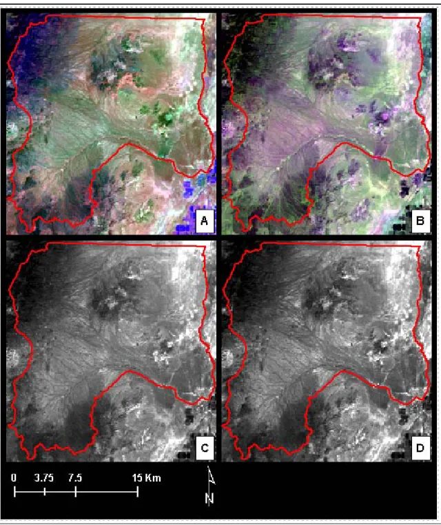
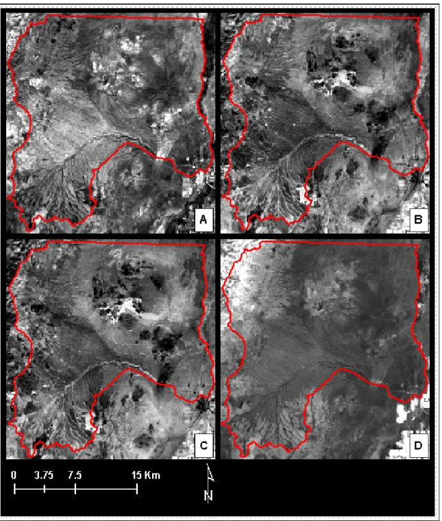
Figure 5. Landsat 7 ETM+ imagery. A: False color composite of bands 5 (red), 2 (green), 4 (blue); B: False color composite of bands 3 (red), 7 (green), 1 (blue); C: band 1; D: band 2.
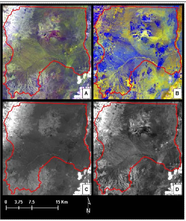
Figure 7. Normalized difference ratios of Landsat 7 ETM+ data. A: False color composite of ratios (4-7)/(4+7) (red), (4-5)/(4+5) (green), (4-3)/(4+3) (blue); B: false color composite of ratios (5-2)/(5+2) (red), (5-1)/(5+1) (green), (4-7)/(4+7) (blue); C: ratio (4-3)/(4+3); D: ratio (4-5)/(4+5).
Figure 8. Normalized difference ratios of Landsat 7 ETM+. A: ratio (3-7)/(3+7); B: ratio (5-2)/5+2); C: ratio (5-1)/(5+1); D: ratio (4-7)/(4+7).
Figure 9. Normalized difference ratio of Landsat 7 ETM+, (3-1)/(3+1).
Digital Elevation Model-Derived Data
Two raster DEM from the national elevation dataset were obtained from the Utah Automated Geographic Reference Center (AGRC, 2008; Figure 10A); one at 9.19-m grid cell resolution (referred to as the 10-m DEM) and another at 30-m resolution. The terrain analysis software, TauDEM (a toolbar addition for ArcGIS), was used to fill sinks in the 10-m and 30-m DEM data sets (Tarboton, 2005). The 10-m DEM was the highest resolution dataset obtainable at the time and offered the most detailed representation of the landscape.
An 11x11 low pass filter was applied to the 30-m DEM to add spatial context to each pixel. For example, consider two pixels that each has a slope of 10 percent: one is on structural bench perched on a steep mountain side and the other is on a small rise on gently sloping fan piedmont. By taking the average across the 330 m by 330 m area the
general slope of the landform that each of these pixels are found on can be determined from this filtered 30-m DEM layer.
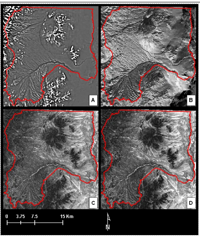
The flow direction raster was calculated from the 10-m DEM using TauDEM (Tarboton, 1997; Figure 10B), which uses the d-infinite algorithm in the slope algorithm. TauDEM was also used to calculate slope for both the 10-m DEM (Figure 10C) and the filtered 30-m DEM (Figure 10D). An ArcToolbox Spatial Analyst tool was used to calculate curvature of the filtered 30-m DEM (Figure 11A). Compound topographic index (CTI) was derived from the 10-m DEM and the flow direction raster using an ArcInfo avenue script (.aml) (Evans, 2004) (Figure 11C). A 5x5 low pass filter was run over the original CTI to produce an additional filtered CTI layer (Figure 11D).
Aspect and elevation were derived from the 10-m DEM . Aspect was
calculated in degrees (0-360º) then transformed to a range of -π to π, where north is –π,
south is π, and east and west are equal to 0 (Figure 11B):
(
)
(
)
° ≤ ° ≤ ° × ° ° − ° ° ≤ ° < ° × ° ° − ° − = ° = 180 0 90 / 90 360 180 90 / 270 1 0 / Aspect if Aspect Aspect if Aspect Aspect if S N Aspect d Transforme π πThis transformed aspect is essentially a measure of northness vs. southness. While there are microclimatic contrasts in microclimates between east- and west-facing slopes (aspect = 0), north- and south-facing slopes exhibit more pronounced differences in soil
Figure 10. DEM-derived data.A: 10-m DEM; B: Flow direction from 10-m DEM; C: Slope from 10-m DEM; D: Slope from the filtered 30-m DEM.
Figure 11. DEM-derived data.A: Curvature from 30-m DEM; B: Transformed aspect from 10-m DEM; C: CTI form 10-m DEM; D: CTI with 5x5 low pass filter from 10-m DEM.
Figure 12. Illustration of the transformation of aspect in degrees to continuous variable of
north-south ranging from -π to π.
Digital Data Exploration and Transformation
Unsupervised and supervised classifications of the digital data using Imagine helped identify patterns used to develop conceptual models and guide field data
collection, and to develop customized data layers used in the random forest classification.
Unsupervised classification requires no a priori knowledge of the study area because it is
completely driven by the digital data.Class means and clusters are found with the
Iterative Self-Organizing Data Analysis Technique (ISODATA). Each pixel is initially assigned to a cluster based on the spectral distance in feature space to the nearest cluster center (mean). Once each pixel has been assigned, a census of each cluster is made. Based on the average pixel value from the census in each cluster, the cluster center is shifted to the new cluster mean to reflect the membership. Once again, all pixels are
assigned to the nearest cluster center. This process is recursive, being reiterated until a user specified convergence percentage is reached or a specified number of iterations have been run. The convergence percentage refers to the percentage of pixels that do not change membership, e.g., when 95% convergence is reached, 95 % of the pixels did not change membership after the cluster mean was recalculated (Leica, 2005). Spectral signatures that are identified can be refined using supervised classification. Supervised
classification requires a priori knowledge. Cluster means for the concept are calculated
from the pixel(s) in a training site, which can be a point or a polygon.
Cluster means for classes may also be identified in spectral feature space (2D histogram) (Leica, 2005). When developing classes with the seeding tool, only a few pixels of a given class are sampled. From these pixels, the Imagine software computes the cluster mean of the class from which a parallelepiped is created in n-dimensional feature space. All pixels are then assigned to a class based on Euclidean distance in feature space. In contrast, the user can draw an area of interest (AOI) to select pixels in feature space. The main difference with editing in feature space is that the user is not merely sampling a few pixels of a class but rather the user is literally assigning pixels to a class – essentially this is direct supervision of pixel assignment. One limitation of the feature space analysis is that a multi-dimensional feature space is represented in only 2-dimensions at a time.
Customized Data Layers
Two customized data layers, the Lake Bonneville shoreline and the Xeric-Aridic soil moisture regime (SMR) raster layers, were created to help stratify the study area into
distinct pedo-geomorphic regions. The 10-m DEM was incorporated into both Lake Bonneville and Aridic SMR models. Landsat 7 data was also used in the Xeric-Aridic SMR model.
There were vector representations available of Lake Bonneville (AGRC, 2008), but they were inaccurate, off by several kilometers from the true shoreline (Figure 13B). While many prominent shoreline features (spits, deltas, shoreline scarps) can be clearly seen in aerial photography there were larger surfaces where shoreline features were not evident, making it difficult to heads-up digitize the shoreline.
The Lake Bonneville layer is a simple binary (true or false) raster layer, where surfaces below ancient Lake Bonneville are “true,” and surfaces that remained above the highest lake level, the Bonneville high stand, are “false.” As explained in the Quaternary History and Geomorphology section, the elevation of this shoreline feature ranged from1558.2 m in the south to 1561.9 m in the north. This northward trend was estimated with simple linear regression. Several prominent shoreline features of the Bonneville high stand were identified in the field and with the aerial photography. These points were attributed with the UTM northing and the elevation value from the 10-m DEM. Using Interactive Data Language (IDL) the elevation trend of the shoreline was estimated to be
1.99x10⁻⁴ m rise in elevation per meter in distance northward. A 10-m raster representing
the hypothetical surface elevation of Lake Bonneville’s shoreline was created where the elevation was calculated as a function of the northing of each cell center (Figure 13A). All raster cells in the 10-m DEM found to be lower than the Lake Bonneville shoreline trend were assigned “true” as they were below ancient Lake Bonneville. The final output
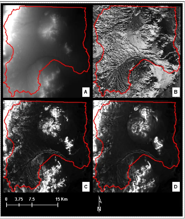
Figure 13. The Lake Bonneville shoreline prediction. A: Hypothetical surface elevation raster of the Lake Bonneville shoreline (gray shading) and the predicted extent of Lake Bonneville (blue). B: Previously available vector layer of the shoreline (red) (AGRC, 2008). Final shoreline output used as a predictive variable in random forests (blue). D: Predicted shoreline feature with linear regression (purple); final edited shoreline (blue).
was vectorized for further editing where minor adjustments (never more than 200 m) were made to match prominent shoreline features (Figure 13C).
The break between xeric and aridic SMR is characterized by single leaf pinyon trees becoming the dominant tree over Utah juniper trees. Spectrally, these two plant communities can be distinguished. Areas of interest (AOI) were delineated over known juniper stands and dominantly pinyon stands in the original Landsat image
(non-standardized). These pixels were then identified in a feature space plot (a two dimensional histogram) of Landsat bands 3 and 4 produced in Imagine. Dominantly pinyon and dominantly juniper stand pixels were found to be in two distinct but contiguous clusters in feature space (Figure 14).
Each cluster was then delineated in feature space (Figure 14) to perform a supervised classification with three general classes: 1) vegetation typical of the xeric SMR, including singleleaf pinyon, fir and others (see vegetation section in Area Description), 2)
woodlands dominated by Utah juniper, which are characteristic of the xeric aridic SMR, and 3) vegetation typical of the xeric aridic and typic aridic SMR, which are
non-woodland or a shrub steppe (e.g. sagebrushes). This output is referred to as the pinyon-juniper (PJ) classification as it was based on the presence of single-leaf pinyon or Utah juniper (Figure 15A).
Not all areas in the xeric SMR are covered by woodland, and areas of irrigated cropland and tamarisk at low elevations in the aridic SMR are spectrally similar to true woodlands at higher elevations. To account for these areas the PJ classification was combined with transformed aspect and elevation in a model (Figure 16). At all aspects, juniper was not observed in the field to occur below 1700 m; also, all farmland and