Structural Performance Comparison of Parallel Software Applications

(1)

Structural Performance Comparison

of Parallel Software Applications

Dissertation

zur Erlangung des akademischen Grades Doktor rerum naturalium

(Dr. rer. nat.)

vorgelegt an der

Technischen Universität Dresden Fakultät Informatik

eingereicht von Matthias Weber, M.Sc. geboren am 8. April 1980 in Cottbus

Gutachter:

Prof. Dr. rer. nat. Wolfgang E. Nagel, Technische Universität Dresden

Prof. Dr. techn. habil. Dieter Kranzlmüller, Ludwig-Maximilians-Universität München Tag der Einreichung: 30. August 2016

(2)

(3)

Acknowledgments

First and foremost, I want to thank Prof. Dr. Wolfgang E. Nagel for giving me the opportunity to work on this subject and for his continuous support over the last years. Also, I would like to thank Prof. Dr. Dieter Kranzlmüller for serving as the second reviewer.

Special thanks are due to Holger Brunst, Ronny Brendel, Kathryn Mohror, and Martin Schulz for their valuable feedback, ideas, and encouragement. Their knowledge and tremendous support improved this work a lot and helped me through the ups and downs of my dissertation work.

Furthermore, I am grateful to Tobias Hilbrich and Ronny Tschüter for their time and effort spent reading my dissertation, and for providing valuable criticisms and suggestions that helped bringing this dissertation into shape.

I also want to thank all of my colleagues and friends at the Center of Information Services and High Performance Computing for a very nice and pleasant working atmosphere that simply made my life better. It has always been fun to go to work over the last years.

Finally, very special thanks go to my beloved partner Claudia and to my mother Christina and brother Bernd-Uwe for their unconditional long term support. If it weren’t for you, the road would have been much more difficult.

(4)

(5)

Abstract

With rising complexity of high performance computing systems and their parallel software, performance analysis and optimization has become essential in the development of efficient applications. The compar-ison of performance data is a key operation required in performance analysis. An analyst may conduct different types of comparisons in order to understand the performance properties of an application. One use case is comparing performance data from multiple measurements. Typical examples for such com-parisons are before/after comcom-parisons when applying optimizations or changing code versions. Besides comparing performance between multiple runs, also comparing performance characteristics across the parallel execution streams of an application is essential to detect performance problems. This is typ-ically useful to detect imbalances, outliers, or changing runtime behavior during the execution of an application. While such comparisons are straightforward for the aggregated data in performance pro-files, only limited solutions exist for comparing event traces. Trace-based analysis, i.e., the collection of fine-grained information on individual application events with timestamps and application context, has proven to be a powerful technique. The detailed performance information included in event traces make them very suitable for performance analysis. However, this level of detail also presents a challenge because it implies a large and overwhelming amount of data. Currently, users need to perform manual comparison of event traces, which is extremely challenging and time consuming because of the large volume of detailed data and the need to correctly line up trace events.

To fill the gap of missing solutions for automatic comparison of event traces, this work proposes a set of techniques that automatically align traces. The alignment allows their structural comparison and the highlighting of differences between them. A set of novel metrics provide the user with an objective measure of the differences between traces, both in terms of differences in the event stream and timing differences across events.

An additional important aspect of trace-based analysis is the visualization of performance data in event timelines. This has proven to be a powerful approach for the detection of various types of performance problems. However, visualization of large numbers of event timelines quickly hits the limits of available display resolution. Likewise, identifying performance problems is challenging in the large amount of vi-sualized performance data. To alleviate these problems this work proposes two new approaches for event timeline visualization. First, novel folding strategies for event timelines facilitate visual scalability and provide powerful overviews of performance data at the same time. Second, this work presents an effec-tive approach that automatically identifies and highlights several types of performance critical sections in an application run. This approach identifies time dominant functions of an application and subsequently uses them to analyze runtime imbalances throughout the application run. Intuitive visualizations present the resulting runtime variations and guide the analyst to performance hot spots.

Evaluations with benchmarks and real-world applications assess all introduced techniques. The effec-tiveness of the comparison approaches is demonstrated by showing automatically detected performance issues and structural differences between different versions of applications and across parallel execu-tion streams. Case studies showcase the capabilities of the event timeline visualizaexecu-tion techniques by demonstrating scalable performance data visualizations and detecting performance problems and code inefficiencies in real-world applications.

(6)

(7)

1 Introduction

This work is centered in the field of High Performance Computing (HPC). Performance optimization of parallel applications is critical in this field to efficiently use available HPC resources. The comparison of performance data is an essential part of this optimization process. Especially the detailed structural comparison of performance data is still very cumbersome and involves manual comparison and alignment of related application sections. This work describes alignment-based solutions for automatic structural comparison of performance data and thereby fills a gap of missing comparison functionalities.

After a short introduction to HPC and performance analysis, this chapter describes open challenges for structural comparison of parallel applications, followed by a summary of the contributions of this work and an overview of the subsequent chapters.

1.1 High Performance Computing

Computers are general purpose devices that can be programmed to execute selected arithmetical and logi-cal operations. Early computers have been large machines filling entire rooms [42,119]. Those machines were available to a limited group of people only, and performed specialized tasks. With rising capability and gradual miniaturization computers have become omnipresent over the last decades. Today, comput-ers are found in many devices surrounding us, such as mobile devices, home appliances, or cars. In the majority of cases small embedded computers are used to carry out dedicated tasks. Also very common are general purpose computers, found in laptops or workstations. Besides building small devices and gen-eral purpose computers, humans always have been putting great effort into creating the most powerful computers possible with currently available technology. Such machines, so-calledsupercomputers, still fill entire rooms today. The computer itself along with the required supporting machinery for cooling, power supply, etc. usually require a dedicated building. With the capability of executing large numbers of operations as fast as possible, supercomputers are employed to solve complex and computationally intensive problems. The field of high performance computing (HPC) refers to all activities related to supercomputers, from the development of software to the design and construction of supercomputers. In the last few decades, HPC has been a critical factor for achieving and preserving scientific and economic competitiveness.

Main driver for HPC over the last 50 years has been an exponential increase in computational speed. This growth, related with Moore’s Law [102], has been accompanied with a continuous increase of memory and storage capacities. This enormous increase of available computing power has enabled unprecedented advancements in science and engineering.

One example are simulations that try to model nature as accurately as possible. Over the years, sim-ulations have become increasingly powerful and complex. Continuous improvements included higher model resolution, longer simulation time, and incorporation of more sub-models. Figure 1.1 gives an example showing the enhancements of climate simulations in the last decades.

Today, computational simulation is established as the third pillar of scientific methodology alongside theory and experiment. Simulations of physical, biological, and chemical processes allow insight when experiments are too expensive, dangerous, or infeasible. Famous examples of such simulations are the computation of molecular interactions in stars or simulations of the earth’s climate covering time spans of tens of thousands of years.

Besides improvements to existing applications, the growth of available computing power made new application domains possible. Application fields such as computational genomics or bioinformatics had been considered infeasible two decades ago. Nowadays, supercomputers are used to solve problems in

(10)

1 Introduction

Figure 1.1: History of horizontal resolution and complexity in climate models used for century scale simulations. The image on the left depicts the increase of the horizontal resolution used in climate models during the last decades. The image on the right lists the components of the Earth system added to climate models during the last decades [80, 139].

various fields, including physical simulations, oil and gas reservoir exploration, molecular modeling, or quantum mechanics. Moreover, scientists already anticipate steady improvements in compute capability to generate scientific advancements.

To satisfy the need for more computing power, ever-more powerful machines have been developed. As described by Moore’s Law the ever-shrinking cost of transistors combined with engineering advances of the processor vendors resulted in an exponential performance improvement of microprocessors. First, this performance improvement resulted directly in higher processing speeds of the microprocessors. On the software side, this effect resulted in direct performance improvement by simply upgrading the hard-ware. Then, in the beginning of the 21st century, physical limits inhibited further advancement of the clock speeds. Since then, additional transistors (which are no longer exclusively used for performance improvements of a single processor) have been used to build extra processors. This change resulted in an ever-increasing amount of parallelism in supercomputers. Figure 1.2 shows an example of the increasing parallelism using the last two supercomputers at the Lawrence Livermore National Laboratory (LLNL), USA. In four and a half years the parallelism between both systems increased by a factor of 7.4. In ad-dition to the rising parallelism, today’s supercomputers increasingly utilize hardware accelerators. The systemTianhe-2 at the National Super Computer Center in Guangzhou, China—No. 1 on the TOP500 list from June 2013 to November 2015—is a hybrid system consisting of 32,000 Intel Xeon processors and 48,000 Xeon Phi accelerators resulting in a total of 3,120,000 compute cores [131].

Increasing heterogeneity and parallelism result in rising complexity of HPC systems. Since almost all computing power improvements of current supercomputers stem from increased parallelism, applications need to exploit parallelism to achieve higher performance. However, the complexity of parallel programs is much higher than the complexity of sequential programs. Due to the current trend of rising complexity in both hardware and software, writing efficient parallel applications gets increasingly harder. Thus, performance analysis is necessary to efficiently exploit HPC systems.

(11)

1.2 Performance Analysis and Optimization

IBM BlueGene/L – 212,992 cores No. 1 on TOP500 list (November 2007) Linpack Performance: 478.2 TFlop/s [131]

IBM BlueGene/Q – 1,572,864 cores No. 1 on TOP500 list (June 2012)

Linpack Performance: 17,173.2 TFlop/s [131] Figure 1.2: Comparison of the last two IBM BlueGene systems installed at Lawrence Livermore National

Laboratory (LLNL). Both systems reached No. 1 in the TOP500 list of the world’s fastest supercomputers in November 2007 and June 2012, respectively. Compared to the four and a half year older BlueGene/L system the current BlueGene/Q system provides substantially increased parallelism and computing power [81].

1.2 Performance Analysis and Optimization

HPC systems provide a theoretical peak performance in terms of floating point rate. However, as the name theoretical suggests, actual production codes achieve only a fraction of that performance in prac-tice. Even highly optimized benchmark codes with considerable adaption for an individual system fall short of achieving theoretical peak performance. The Linpack benchmark [30], widely used to measure performance of HPC systems, primarily achieves only about 60%-85% of the theoretical peak perfor-mance across top 10 systems [29, 131]. Real scientific applications usually achieve less sustained per-formance. For instance, highly optimized applications, nominated for the Gordon Bell Prize—an award presented yearly for outstanding achievements in HPC applications—achieve only 55%1or 26%2of the theoretical peak performance. Yet, for the majority of scientific applications their fractions are even below these numbers.

The performance optimization goal is to achieve as much of the theoretical peak performance as pos-sible. However, this is no trivial task. The first viable part is to design and implement computationally efficient code, e.g., by choosing the best performing algorithm for a given problem. The second viable part to increase efficiency is to adapt the software to the particular hardware. Yet, modern computing systems are very complex, due to the addition of numerous performance optimization techniques. Cur-rent systems may include complex memory access behavior via multi-level caches, pipelined instruction execution (including complex dependencies), branch prediction, speculative execution, and parallel exe-cution features. All of these concepts provide considerable performance gains. However, failing to fully utilize any one of these concepts will result in loss of a noticeable fraction of the theoretical peak per-formance. Additionally, HPC machines are usually individual systems that require individual adaption strategies. The top HPC systems are replaced every three to five years with new systems, that may exhibit significant architectural differences. Thus, performance optimization of parallel software is a continuous and challenging task.

HPC systems exhibit a high degree of parallelism. Applications need to exploit that parallelism to fully utilize available resources. Therefore, the calculated problem is split up into sub-tasks (parallelization)

1

11 PFLOP/s Simulations of Cloud Cavitation Collapseon the IBM Blue Gene/Q systemSequoia[120].

2

(12)

1 Introduction

that are distributed across the available processing cores of the parallel machine. ThespeedupS then describes the relative performance improvement. In theory, the ideal parallelization of an application would result in a linear speedup, i.e., an application divided into ten parts computed in parallel on ten compute cores should run ten times faster than its sequential version on one core. However, due to synchronization and data dependencies, it might not be possible to parallelize all parts of an application. For instance, a simulation may first need to load input data before it can start with parallel calculations, or some calculations may require results of other calculations. In such cases, according to Amdahl’s Law [5], the sequential fraction of the application limits the maximal possible speedup. An alternative approach, suggested by Gustafson [50], to measure parallel performance improvement, is to increase the problem size along with rising compute core counts. An application version computing a problem twice the size than the initial version, on twice as many processors should still require the same runtime as the initial version. However, applications rarely achieve ideal speedups. Usually, with rising process counts and problem sizes, the relative performance improvement decreases. Consequently, thescalability of an application describes in general how well it can exploit parallelism to reduce its runtime and to compute larger problem sizes. Efficient parallelization of codes is no trivial task. The degree of scalability for an application highly depends on the possibilities of partitioning the underling problem. In the easiest case, the problem can be split up into many independent sub-tasks. In practice, HPC systems often solve problems that can only be separated into sub-tasks that depend on each other. For instance in climate simulations the simulated area is split up into small blocks. Each processor calculates the climate in its block. For the calculation of its block each processor additionally needs the results from the neighboring blocks. The dependence between sub-tasks introduces the need for communication. This dependence also requires synchronization between sub-tasks. Ideally, the problem is split up into completely equal sub-tasks. In practice, this is rarely possible. Using the example of a climate simulation: Even if the block sizes are completely similar, the individual workload also depends on the simulated weather conditions inside the block. As a result, some processes (calculating “faster” blocks) will need to wait for the result of other processes (calculating “slower” blocks) before they can continue with their computations. Consequently, communication and synchronization can severely limit scalability and thus reduce application efficiency.

To evaluate how good an application is adapted to the available hardware and how efficient the par-allelization is implemented, performance analysis is necessary. Yet, to assess the performance of an application and to identify performance problems, it is not sufficient to merely measure the application’s execution time. Application runtime alone reveals only few details about the complex execution behavior of parallel applications. Performance problems can have multiple causes that may be related to sequential and parallel behavior of arithmetic operations, memory accesses, I/O, communication, synchronization, and load balancing. Users require detailed insight into the application runtime behavior to reasonably evaluate the application’s performance. However, the complexity of many HPC applications renders a manual analysis cumbersome at best. For instance some HPC applications, like Trinity [55, 136] (a tool for de novo reconstruction of transcriptomes from RNA sequencing data), consist of a set of linked inde-pendent software components. Each component represents an own application itself. Results are passed from one component to the next. It is not unusual that components programmed in different programming languages or using different parallelization paradigms are linked together. The components in Trinity are programmed using C++, Java, or Python. The code connecting all components of Trinity is written in Perl. To evaluate the performance of such applications, analysts first need to find a way to measure how individual components contribute to the overall application runtime. Ideally, analysts need to assess more parameters, like the effectiveness of the parallelization and the memory consumption of each component. Then, after this initial analysis, promising components for performance analysis can be chosen. Only af-ter this step starts the actual search for performance bottlenecks of individual components. Then, afaf-ter performance problems are detected and fixed, the optimized component’s performance and the complete application’s performance need to be compared to the performance of the initial application version. Manually conducting and analyzing these numerous measurements is challenging and time consuming.

(13)

1.3 Challenges for Performance Data Comparison Performance data Performance data Perform changes Analyze performance impact of changes Application run: n Application run: n+1

Figure 1.3: Performance optimization is a repeating process.

Therefore analysts rely on performance analysis tools to support and alleviate their work. These tools manage measurements throughout the application’s execution and visualize the recorded data in profile and timeline charts. Profiles provide a statistical overview of performance critical parts of an application. Timeline visualizations allow insight into dynamic runtime behavior. Analysis of this performance data allows users to evaluate individual application executions and to find potential code sections for optimiza-tions. Moreover, detailed performance data of an application run allows to detect complex performance issues and to identify causes of insufficient performance. Typical HPC applications do not pose the prob-lem of comprehensively analyzing multiple linked components. They usually consist of only a single binary that is executed with a high degree of parallelism. When optimizing such applications, the user needs to analyze the behavior of hundreds of thousands of processes [37, 150, 151]. Manually conduct-ing and analyzconduct-ing measurements for such applications is not feasible anymore. Analysts require tools to manage and process large-scale measurements. In fact, it is challenging for performance analysis tools also, to keep up with the scale of applications and still produce meaningful results [150]. The amount of measurement data increases along with application scale. In order to support large scale applications, analysis tools need to improve and adapt their underlying technology [78]. To provide meaningful vi-sualizations of large data sets, tools cannot afford to simply visualize everything, but need to focus on relevant information [91].

1.3 Challenges for Performance Data Comparison

Performance optimization is usually an iterative process. As depicted in Figure 1.3 users first start with an initial measurement as a baseline for comparison. Then, they try to find and optimize inefficient parts of an application and conduct a new measurement. A comparison of the two measurements shows the effect of the optimization. Depending on the result of the comparison, the user may choose to change or add new optimizations and conduct new performance measurements for further comparisons. Without such comparisons, it is challenging to evaluate the performance impact of applied changes. Consequently, comparison of performance data is a key operation in performance analysis. Scenarios for comparisons include:

• Before/after comparisons when applying optimizations or changing code versions,

• Comparisons of runs on different platforms to study performance portability, and

• Contrasting the performance of different processes to study load balance or synchronization delays. Performance data is usually stored in form of profiles or traces. Profiles aggregate data during col-lection and provide an overview of the performance of an application. In principle, profiles consist of a list of numbers. Each number describes the performance of a specific part of the application, typically a function. This renders the comparison of profiles rather straightforward as related numbers can be compared directly. Numerous tools already support the comparison of profiles [63, 124].

(14)

1 Introduction

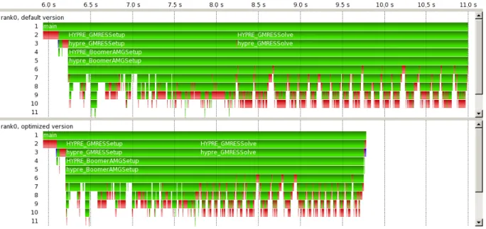
Figure 1.4: Manual visual comparison of two processes. The two timelines contrast a run of the default version (top) with an optimized version (bottom) of an application.

A trace is a sequential record of application behavior. Each application activity, e.g. entering or leaving a function, or sending a message from one process to another, is stored as time-stamped events. Traces allow in-depth insight into the performance behavior of an application. They are especially useful for detecting root causes of performance problems with temporal components. However, the comparison of traces is a challenging task due to the possibly large amount of complex performance data recorded. Figure 1.4 gives an example for this situation. The figure shows two timelines. Each timeline visualizes the trace data recorded on one process (the execution stream running on one compute core) of a parallel application. The top timeline shows a run of the initial version of the application. The bottom timeline shows a run of the optimized version of the application. Each timeline consists of multiple horizontal bars labeled with numbers on the left side. The numbers show the call level of the respective horizontal bar. The colors represent executed functions on the process. Red colors relate to MPI [103] functions (a library providing functionality for communication and synchronization between processes), while green colors relate to functions of the application code. When visually comparing both timelines, it is obvious that the optimized version runs faster than the initial version. The bottom timeline is shorter than the top timeline, thus the optimized version of the application finishes earlier. However, detailed structural differences or performance differences throughout the application run are not immediately visible. To see details, the analyst needs to manually compare both timelines. As the bottom timeline is shorter than the top timeline, related application areas do not appear above each other. For a detailed comparison, the analyst needs to manually align the timelines in order to compare related events. However, manual comparison is extremely challenging due to the large number of events and the need to correctly line up trace events. This renders this task cumbersome and error-prone. Analysts require automatic support for event-wise trace comparison. This dissertation helps to improve this situation by providing automatic alignment-based comparison methods for trace data.

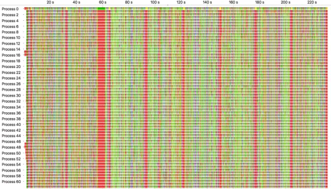
A similar situation arises when comparing multiple processes of a parallel application. Figure 1.5 demonstrates such a comparison case. The figure shows 63 timelines, representing individual application processes. The colors in the timelines represent different functions invoked on the processes. Visible are eight iterations, separated by red vertical blocks. The application invokes MPI calls for communication and synchronization in that area. Each process executes several different functions during its iterations, as the colors between the red areas suggest. Judging if all processes execute the same sequence of functions in their iterations is a tedious task when relying on manual analysis alone. Clearly visible

(15)

1.4 Contributions

Figure 1.5: Manual visual comparison of multiple processes of one application run.

is that the first process executes different functions than the other processes. But exactly quantifying other differences between processes is time consuming and error-prone. An additional difficulty pose time-shifts and different function durations between the processes, that cause related functions to appear at different horizontal positions between processes. Correctly performing such an analysis manually for larger process counts is almost impossible. To alleviate this task, this work introduces methods that allow an automatic structural comparison of multiple processes.

1.4 Contributions

The comparison of the structure of processes currently needs to be performed manually. Users have to align related events by hand and are required to compare large numbers of events. This work introduces methods that alleviate this cumbersome task for users. Automatic analysis methods allow fast structural comparisons of processes and build the basis for subsequent detailed performance comparisons between processes. This work provides missing functionalities for the task of comparing performance data and additionally introduces novel approaches for the visualization of event timelines. The following contri-butions are made.

1.4.1 Structural Comparison of Process Pairs

This work introduces a method to compare the event streams of two processes [140]. Based on algo-rithms from bioinformatics a fast hierarchical sequence alignment algorithm is developed. The novel hierarchical algorithm exploits the function call structure of a process to speed up the required alignment time. With this performance improvement, the alignment, and thus, structural comparison of processes becomes feasible. The introduced hierarchical sequence alignment algorithm allows a detailed detection of equal and differing areas between two processes.

(16)

1 Introduction

1.4.2 Alignment-Based Comparison Metrics

Based on the novel hierarchical alignment algorithm, new comparison metrics are introduced [144, 145]. These metrics include a definition of the structural similarity between two event streams and provide fine-grained insight into structural and temporal differences between two processes. A case study, applying the alignment-based metrics for the comparison of different versions of several applications, demon-strates their potential for the comparison of parallel applications. The metrics exposed differences that otherwise would have been hard or even impossible to find.

1.4.3 Structural Comparison of Multiple Processes

A new scalable clustering approach enables grouping of large numbers of processes according to their structure [141]. This novel grouping approach for processes has linear time complexity and results in a low number of clusters for many application types. The method is designed as a pre-clustering step for subsequent detailed analysis techniques.

A novel hierarchical multiple sequence alignment algorithm that is capable of aligning large num-bers of processes is introduced. Using the pre-clustering result, the algorithm compares processes of one cluster in detail and thereby identifies structural differences and similarities. Key components pro-viding the algorithm speed are the hierarchical approach and a new heuristic that evaluates structural similarity between processes. The algorithm computes a compact data structure, a so-called merged call tree, that combines the structural information of all compared processes and provides rich potential for performance analysis.

1.4.4 Visualization Techniques for Event Timelines

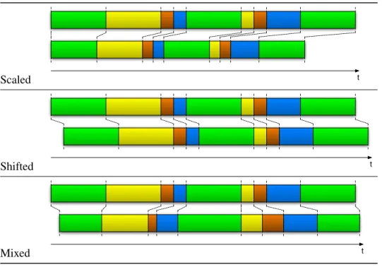
New visualization methods for the analysis and comparison of event timelines are introduced. By applying different folding strategies for timelines, scalable visualizations that facilitate easy detection of performance problems and provide condensed overviews of the performance behavior are demon-strated [142].

Additionally, this work introduces an analysis approach based on performance variations [143]. The approach automatically identifies and highlights performance critical sections. The visualization of per-formance variations is applicable to guide analysts in the task of identifying perper-formance bottlenecks.

1.5 Organization of This Dissertation

Chapter 2 explains the theoretical background of this work and describes related work. It identifies missing functionalities for the comparison of performance data. Chapter 3 provides solutions for the pairwise structural comparison of two processes. Event streams of two processes are compared using alignment techniques. Chapter 4 introduces performance metrics based on the pairwise alignment tech-niques described in Chapter 3. The effectiveness of introduced metrics for the comparison of processes is demonstrated in a case study with two applications and one benchmark. Chapter 5 provides approaches for the structural comparison of multiple processes. In a first step, processes are clustered based on their structural information. Then, for detailed comparison, processes of a cluster are aligned using multiple sequence alignment methods. Chapter 6 introduces novel techniques for the scalable visualization of performance data and automatic highlighting of performance hot spots. Chapter 7 summarizes this work and shows possible directions for further developments.

(17)

2 Background and Related Work

Performance analysis of software is getting increasingly important. This is especially true for the field of high performance computing (HPC). Rising complexity of both hardware and software requires per-formance analysis and optimization for the efficient exploitation of current high-end systems. Inefficient applications may waste valuable resources or may only provide reduced capacity due to performance bottlenecks. Consequently, considerable effort is put into performance analysis technology.

This chapter introduces fundamental concepts and tools for performance analysis. It discusses tech-niques related to performance data comparison and puts a special focus on automatic analysis and com-pression methods for trace data. It concludes with an analysis of discussed techniques in regard to trace file comparison and lists missing functionality required for a comprehensive comparison of parallel ap-plications.

2.1 Measurement of Performance Data

This section introduces fundamental techniques for the measurement of performance data and discusses trade-offs associated with them.

The performance analysis of an application requires measurements at application runtime. For accu-rate time measurement systems provide hardware support by high-resolution timers offering precision in the microsecond or nanosecond range. Besides timers, most systems also provide additional hardware performance counters. Such counters may count events like floating point operations, cache misses, instructions, or branch mispredictions.

In order to use hardware counters for measurements, instructions need to be inserted into the applica-tion’s control flow. This modification can be implemented in several ways.

The first major method to acquire performance data is calledinstrumentation. Instrumentation tech-niques insert measurement instructions directly into the control flow of an application itself. That way the instructions will be performed in the course of the application’s execution. Such inserted instructions may measure time intervals using high-resolution timers or collect values from hardware counters. There are three common techniques used to implement this method of performance data acquisition.

• Source code instrumentationadds measurement instructions to the source code of an applica-tion. In this way measurement routines are compiled together with the original application code. Usually, this is the first approach used by programmers to debug an application or to produce per-formance measurements by manually adding instructions to print data or timings to the screen. For the instrumentation of larger code projects, tools that automatically insert measurement in-structions into the source code may be used.

The disadvantage of source code instrumentation is that included measurement instructions are always executed. In order to dynamically enable and disable individual measurements, guard statements need to be placed around measurement instructions. Consequently, even disabled mea-surements will cause some perturbation during the application execution.

• Binary instrumentationadds measurement instructions directly into the application’s object code. This saves recompilation of the application. During runtime instructions for measurement are ex-ecuted along with application instructions. Typically, measurement instructions are inserted into an application’s object code by the usage of so-calledtrampoline functions. A trampoline function is an unconditional jump that transfers control to the measurement code that itself performs the actual measurement and returns control back to the application.

(18)

2 Background and Related Work

Instrumentation: Sampling:

t

Figure 2.1: Sampling and instrumentation. Both methods differ primarily in the way the measurements are triggered. Colored timelines indicate a series of executed functions. Black arrows below the timelines indicate measurements. In case of sampling, measurements are triggered at periodic time intervals. In case of instrumentation, measurement instructions are embedded into an application’s control flow and triggered at function begin and end points.

An advantage of binary instrumentation is that filtered/disabled measurement instructions can be dynamically removed from the object code. Thus, filtered measurements do not induce overhead as they are never executed.

• Link-level instrumentation uses the linker to insert measurement instructions into an applica-tion’s control flow. If an application uses libraries, its calls to these libraries are resolved by the linker. When using link-level instrumentation, awrapper library that implements wrappers for function calls of the target library is linked together with the application. Calls to the target library will first resolve to measurement routines in the wrapper library and then pass on to the target library.

For statically linked libraries re-linking of the application is necessary. With dynamically linked libraries, it may be possible to load the wrapper library at the application launch, e.g., via the LD_PRELOADenvironment variable in Linux.

The second method of performance data acquisition is calledsampling. Sampling issues measurement instructions asynchronously. Measurement instructions are not embedded into an application’s control flow but triggered at periodic time intervals. For this purpose most operating systems provide interrupt handlers that interrupt an application’s execution at a regular time interval. At each interrupt samples describing where an application spends its time or what resource it uses are taken. Sampling does not require any re-compiling or re-linking and can be directly used with the unmodified application binary.

Besides the different implementation approaches, both methods differ primarily in the way the mea-surements are triggered. Figure 2.1 depicts the difference between sampling and instrumentation. This difference induces inherent advantages and disadvantages for each method. Instrumentation measures all events as they occur in runtime, since measurement instructions are embedded directly into an appli-cation’s control flow. An instrumented function is guaranteed to be observed each time it is executed. This ensures a complete coverage. With sampling, as measurements are triggered at asynchronous time points, there is no such guarantee.

In case of instrumentation the amount of measurement overhead depends on the specific application and on how often instrumentation code is executed. The instrumentation of frequently called, short run-ning functions can induce a high perturbation to an application. Typically, individual functions causing a high measurement overhead need to be filtered. Depending on the method of instrumentation, even filtered functions may cause measurement overhead. In case of sampling the measurement overhead is controlled by the sampling rate. A fixed sampling rate allows to exactly estimate the overhead prior to the measurement. The chosen sampling rate is a trade-off between overhead and sampling error. If the sampling rate is too low, infrequent or short events can escape observation. If the sampling rate is too high, an application can be perturbed severely.

(19)

2.2 Performance Analysis Tools

Timeline Profile Data

t Execution Time Fractions Execution Time per Function

t Trace Data

Figure 2.2: Profile and trace data representations. A colored timeline at the bottom indicates a series of executed functions. Trace data allows the complete reconstruction of an application’s execution. A typical timeline generated from trace data, indicated at the bottom, displays the complete execution. Profile data aggregates information and provides statistics about an application’s execution. Indicated at the top, profile displays present function statistics of the application run indicated at the bottom.

Recorded measurement data is typically stored employing aprofileor atracedata format. Figure 2.2 depicts typical performance data representations generated from profile and trace data respectively. Pro-files are an aggregated record of an application’s behavior. Due to the data aggregation this approach is scalable. However, the data aggregation also limits the analysis potential of this technique. Perfor-mance problems occurring dynamically might not be visible in profile perforPerfor-mance data. Profiles are typically used for an overview or a first analysis of an application’s performance characteristics. A trace is a record of an application’s behavior as a series of events, such as function entry and exit, or message passing. Each event consists of a time-stamp along with relevant data, e.g., function name, or bytes of data transmitted. The detailed information included in traces make them very suitable for detection of many performance problems on HPC systems, e.g., the causes of synchronization delays. However, the level of detail also presents a challenge because it implies a large amount of data from a single run, even exceeding hundreds of megabytes for a single process [97]. A common approach to cope with large trace sizes is to use filtering mechanisms to exclude irrelevant information.

2.2 Performance Analysis Tools

Performance optimization is required to fully exploit available hardware and for the design of efficient code. Often the first step in understanding an application’s performance behavior is to manually instru-ment some parts of the application with available timer calls, likegettimeofdayon Linux systems, and print the results to the screen. The drawback is that this method only measures user selected code sections and provides no overview of the complete application’s performance characteristics. This man-ual approach is prone to miss important performance information. Also, manman-ual instrumentation tends to be cumbersome, especially with rising code complexity. When analyzing parallel software the man-ual approach becomes even more involved and the results are harder to analyze. To assist the analyst in this cumbersome task a large number of performance analysis tools have been developed. The tools automate the measurement process, using one or a combination of the above described performance data

(20)

Figure 2.3: Example of a flat profile generated by gprof [33]. The table is ordered by the percentage of the total execution time spent in individual functions. The profile provides additional information about the time spent in respective functions and their number of invocations.

acquisition methods, and provide convenient representations of the performance data. Depending on the employed measurement technology and the corresponding performance data representation these tools divide into two major groups.

Profilers The best-known group of performance analysis tools consists ofprofilers. A large number of profiling tools are available and basic profilers are often pre-installed on most operating systems. One example of a common profiler is gprof [33, 47]. gprof is distributed along with Linux/Unix systems. The key characteristic of a profiler is the aggregation of the measured performance data. This data aggregation results in a profile, hence the name profiler, providing an overview of the performance characteristics of the measurement run. Looking at a performance profile the developer can quickly identify performance critical parts during an application’s run. For instance a profile may list the most time consuming functions that thereby present good candidates for performance optimization. Typical representations of a performance profile use bar or pie charts as well as tables, see Figures 2.2 and 2.3.

Figure 2.3 depicts an example of a flat performance profile represented in a table view. A flat profile typically presents average times and frequencies of functions measured during an application run, ignor-ing the caller-callee relationship of functions. In addition to flat profiles most tools, e.g., gprof [33, 47], Intel VTune Amplifier [64] or AMD CodeXL [4], also support call-graph profiles. A call-graph profile presents average times and frequencies of functions broken down by the call-graph based on the callee.

Profilers use sampling or instrumentation techniques to measure performance data. Like in case of gprof, also hybrid approaches of sampling and instrumentation are employed. Depending on the measurement system profilers may also be able to aggregate performance data from multiple execution streams. This data aggregation provides a scalable method for performance data storage and presentation. Consequently, a range of profilers focusing on the analysis of multiple processes has been developed in the field of parallel computing. These parallel profiles also employ sampling as well as instrumenta-tion techniques. Examples of parallel profilers using sampling are Allinea MAP [2], HPCView [90], or HPCToolkit [1]. Profilers employing the instrumentation approach are, e.g., Cube [129], TAU [9, 61], mpiP [135], or Paradyn [92]. Like shown by Open|SpeedShop [125], also combinations of both tech-niques, sampling and instrumentation, are employed by parallel profilers.

Usual performance profiles present aggregated data of the complete application run. To achieve a more detailed and differentiated view of the performance behavior, some tools employ a technique called phase-based profiling. The phase-based technique splits the application execution into separate phases. Figure 2.4 shows a phase-based profile generated by TAU [89]. In the depicted example three

(21)

2.2 Performance Analysis Tools

Figure 2.4: Phase-based profile showing individual profiles for x, y, and z solver phases. The top view shows the three phases in a compound way. Functions occurring outside the phases are shown separately. The bottom view shows detailed information for each individual phase. [89] individual phases for the solver have been defined, i.e., y_solve_phase, z_solve_phase, and x_solve_phase. For each phase performance data is aggregated individually. Hence, the applica-tion is characterized by multiple profiles, each representing an individual phase. This approach allows a distinct performance analysis of individual code sections.

Tracing Tools Tracing toolsform the second group of performance analysis tools. These tools allow the most detailed analysis of an application’s performance behavior. Contrary to the data aggregation applied by profilers, tracing tools keep all recorded performance data. During the course of an applica-tion’s execution its behavior is recorded as a stream of events. Additionally to event specific data, like function name or bytes of data transmitted, each event also includes a time stamp indicating its time of occurrence. Tracing tools use this record of events, the trace file, to visualize and analyze the applica-tion’s behavior. Especially the preservation of all timing information allows the detailed reconstruction of application executions. Moreover, the full timing information is required for the analysis of dynamic performance behavior. For instance, dynamic load imbalances can severely limit performance of parallel applications [13]. Consequently, for performance analysis traces are more powerful than profiles and enable the detection of many performance problems critical to HPC applications.

In order to measure performance data tracing tools employ the methods described in the previous section. Many tools use instrumentation, e.g., Vampir [18, 106], Intel Trace Analyzer and Collector [63], or Jumpshot [28, 149, 152]. Also sampling is applied by some tools, like for instance Paraver [112] or HPCToolkit [1].

Tracing tools typically use timeline views to illustrate the behavior of parallel applications, see Fig-ure 2.5. Timeline views depict the state of each process at any point in time along with the communication between processes. Additionally to process states also performance metrics like values from hardware performance counters may be visualized in timeline views.

Besides timelines tracing tools also compute profiles from event data. In contrast to profiling tools where the profiles cover either the complete application run or defined application phases, the computa-tion of profiles from trace data is more flexible. Due to the timing informacomputa-tion included in each stored event, profiles can be computed for arbitrary time intervals.

(22)

Figure 2.5: A timeline view showing a simple ring program executed with eight processes. Each process is depicted as a separate timeline. One message, indicated by white arrows, is passed from one process to the next until it arrives back at the initial sender process. [152]

In addition to performance data visualization some tools provide automatic analysis features. For in-stance Jumpshot [152] provides detection of function invocations with irregular durations. The detection is driven by the assumption that all invocations of a particular function should run for approximately the same period of time. Using a normal distribution in combination with a high and low cutoff, Jump-shot identifies function invocations with irregular durations. Other examples are Scalasca [38, 148] and Periscope [11]. Both tools automatically detect wait states in parallel applications due to inefficient communication behavior.

The trade-off for more detailed analysis capabilities is a larger volume of performance data. To cope with the possibly large amount of performance data most tools apply filtering methods to exclude ir-relevant data. Additionally to filtering, the Vampir tracing framework provides a parallel analysis en-gine [17, 19], allowing to harness the power of a distributed system for the performance data analysis.

2.3 Analysis and Comparison Techniques

This section provides an overview of analysis techniques for event traces. Additionally, it introduces comparison techniques for performance data. First, tools for visual trace comparison are presented. Then tools for management and comparison of multiple measurement runs are discussed. Last, automatic techniques for compression and analysis of event traces are covered.

2.3.1 Visual Event-Trace Comparison

A straightforward method to compare event traces is to manually perform visual inspection. Users can open several instances of one tool, each showing an individual trace for comparison. Yet, this manual comparison is likely to be extremely challenging and time consuming. Since related events may appear in different places, it involves to correctly line up individual trace events. To alleviate this cumbersome task some tools provide a visual comparison mode. This mode shows multiple traces next to each other for easier comparison.

(23)

2.3 Analysis and Comparison Techniques

Figure 2.6: Three different traces displayed in the comparison view of Vampir. The traces are distin-guishable by their background color: white, light blue, and light green. Each trace shows the same application but measured on a different machine. Green and blue areas in the timelines depict functions performing computations. The different lengths of the computing functions indicate unequal performance of the measured machines. [134]

Vampir The comparison view provided by Vampir [19] arranges multiple traces side by side in one central display. To facilitate detailed comparison of selected events, traces can be individually shifted in time. This enables a manual alignment and compensates for varying start times of events, e.g., due to dif-ferent initialization durations in the traces. Figure 2.6 depicts the comparison view showing three traces. Each trace represents the same application but measured on a different machine. The figure displays the traces after manual alignment. The compute iterations are aligned next to each other. The runtime differences between the traces become obvious. Compared to the bottom trace, the computations (blue areas in the figure) are considerably faster in the top two traces. Figure 2.6 also shows the limitations of this approach. In case of high runtime differences it may be hard to display events side by side. As shown in Figure 2.6 the iterations of the middle trace barely consume half of the timeline space while the iterations of the bottom trace do not even fit on the available space.

An approach proposed by Knüpfer et al. [77] is based on C3G, an alternative data structure for trace data. When using C3G the trace data is stored in a tree-like graph. Similar repeated events share the same node in the graph. Hence the graph inherently identifies repetitive patterns. Knüpfer exploits this advantage and visualizes repetitive patterns in one process. This method simplifies the detection and visual analysis of patterns inside one trace. Consequently, this method assists in the visual comparison of patterns between multiple traces as well.

Intel Trace Analyzer Similar to Vampir the Intel Trace Analyzer and Collector [63] also provides support for visual trace comparison. The Intel Trace Analyzer limits the comparison to two traces at a time. It offers two modes of operation. The first mode depicts each trace according to its real execution time. The second mode visually stretches the shorter trace to the length of the longer trace. That way both traces appear to have the same total execution time and related areas are shown approximately next to each other. This type of visual display does not show the real trace timings anymore but may help in the visual comparison process. Additionally to the visual timeline comparison, the Intel Trace Analyzer also computes differences between the profile data of both traces.

(24)

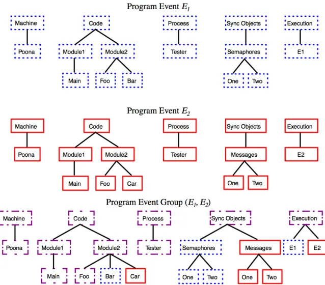
Figure 2.7: Structural comparison of the resource hierarchies of two application executions. EventsE1 andE2describe the first and the second application run respectively. The bottom set indicates similarities and differences in the structure between both runs. [69]

2.3.2 Measurement Management Support

Performance optimization of parallel applications usually involves multiple measurement runs. Typical use cases are comparing results of different optimization strategies or studying application portability when moving from one machine to another. Several solutions for managing and analyzing performance data from multiple measurement runs exist.

Differential Profiling The comparison of profiles from two application executions is an essential performance analysis step that users routinely perform. However, most profiling tools do not provide direct support for this analysis task. Yet, the comparison of profiles is straightforward. Usually, first the differences in function runtimes between two application runs are computed. Then the results are sorted from largest to smallest difference. This allows users to quickly identify the key differences between two application executions, typically by just looking at the top functions in the profile. Schulz and de Supinski provide tool support for this approach in their workPractical Differential Profiling[124]. They introduce an extension of the commonly used profiler gprof [47]. Their tool eGprof facilitates comparisons of two performance profiles inside gprof. The tool allows to “subtract” two performance profiles and provides call-graph visualization of the differences.

(25)

Experiment Management Support More comprehensive functionality allowing the management of multiple application executions provides the framework for multi-execution performance tuning pre-sented by Karavanic [67, 69, 70]. Each execution of an application is considered as an experiment. The framework defines aprogram spacethat gathers all information related to one application. The collected information consists of details about all experiments (application runs) like the components of the code executed, the execution environment, and the recorded performance profile data. An experiment man-agement tool facilitates exploration of the program space. The tool allows analyzing differences between multiple application executions. Displayed differences may regard changes in program source code and the resources used at runtime as well as differences in the application’s performance. Figure 2.7 depicts a structural comparison between two resource hierarchies. The collection of profile data spanning multi-ple program executions additionally allows analyzing the performance evolution of one application. The Paradyn performance tool [92] provides an automated search for performance bottlenecks. The incor-poration of information from the program space into the Paradyn Performance Consultant [60] allowed to guide the tool’s search strategy based on performance data gathered in previous executions. This re-sulted in a more effective diagnosis of bottlenecks. Later work [68] added database technology for more flexible collection and storage of performance data from multiple locations.

An algebra building upon the described framework for multi-execution performance tuning is pro-posed by Song et al. [129]. It provides additional arithmetic operations to merge, subtract, and average data. The algebra is used for cross-experiment performance analysis. It allows comparing, integrating, and summarizing performance data from multiple sources. Sources of the performance data may build multiple experiments of MPI and/or multithreaded applications as well as results obtained from sim-ulations and analytical modeling. The algebra represents performance data in a platform-independent fashion. The algebra output data is presented in the same way as the input data, allowing the use of the same set of tools for visualization.

The PerfExplorer tool [61, 62] provides a framework for performance data mining. Measured perfor-mance profile data is stored in a database and can be processed with data mining methods. Addition-ally to clustering and correlation algorithms also comparative analyses are supported. Runtime, relative speedup, and efficiency can be compared across different sets of profiles. PerfExplorer provides tool support for parameter or scalability studies of an application.

Vertical Profiling A work presented by Hauswirth [52, 53] introduces a technique calledVertical Profiling. The intention is to record and compare numerous metrics for one application. The metrics cover the entire system including, e.g., hardware, operating system, libraries, and application. For each metric a trace is collected. To control the measurement overhead only a limited number of metrics is recorded during a single application run. Therefore, multiple consecutive measurement runs are taken for the collection of all necessary metrics. The recorded traces are subdivided into successive interval parts. For each interval an aggregated profile value is computed. For the comparison and analysis of the metrics all traces are vertically arranged. Due to the inherent jitter in timing measurements the traces need to be aligned prior to the comparison of related interval parts. The alignment is computed using a dynamic time warping algorithm that requires a common metric in each measurement run. This approach only works for traces measured with the same application configuration and in presence of a suitable common metric for the alignment.

2.3.3 Similarity-Based Compression Techniques for Event-Traces

Traces store an application’s behavior as a series of events. Especially the preservation of all timing information enables the detection of a wide range of crucial performance problems. However, this de-tailed information also results in large data volumes. Performance measurements of parallel applications may lead to unmanageably large trace files. Studies investigated the overhead of tracing on parallel systems [94, 95, 97]. One critical cause of overhead is writing of trace data to disk. Periodic flushes of trace data may cause severe perturbation in the target application. Additionally, the overhead for

(26)

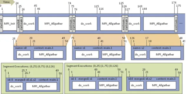
Figure 2.8: Intra-process segment matching scheme. The top bar represents a portion of an example trace with time values indicated above the trace. Segment markers are shown as light gray rectangles. The three resulting segments are displayed below the trace (s0, s1, and s2). In each segment the time stamps are adjusted relative to the segment start time. The bottom row shows two examples of segment matching. In the left example all three segments are merged together. In the right example the threshold is smaller allowing less variation. Hence, the segment s1 is incompatible and only segments s0 and s2 are merged together. [101]

writing strongly depends on the file system speed and increases with rising numbers of processors. Con-sequently, a range of approaches has been developed to compress the trace data at runtime and reduce the data volume required for writing. The compression techniques may target wide traces (large number of processes) and/or long traces (long runtime of the application). In order to achieve high compression rates all techniques aim to exploit similarities. Compression techniques for long traces benefit best from the iterative behavior of many HPC applications by exploiting repetitions in one process. Compression techniques for wide traces are based on the Single Program Multiple Data (SPMD) paradigm and try to exploit similarities across the processes of a parallel application.

Trace Profiling One solution addressing the reduction of overhead of writing traces is trace profil-ing[96, 99–101]. Trace profiling is a hybrid between tracing and profiling. This measurement technique collects summary information about event patterns that occur during program execution. The technique reduces the trace data volume and writes an approximate trace of a complete application’s run. The trace retains enough information to diagnose performance problems that traditionally require traces. The tool Scalasca [148] has been used to evaluate the retention of correct performance behaviors, by comparing automatically detected performance bottlenecks between the original trace and the reduced trace.

To accomplish the data reduction loops are used to partition an application into segments or patterns. The segments build the basis for intra- and inter-process comparison. Segments with the same context (equal patterns) are matched. If they have similar durations within a predefined threshold, only one representative segment is saved. Figure 2.8 depicts the intra-process segment matching scheme. Intra-process segment matching is done at runtime, reducing the data volume written to disk. For effective segment matching a study evaluated several similarity metrics for compression [98]. The study indicated that the average wavelet transform method provided the best trade-off between retention of performance trends and file size reduction.

(27)

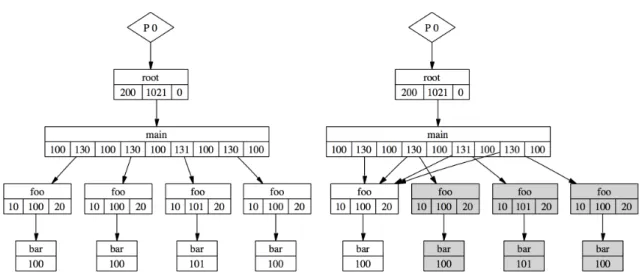
Figure 2.9: Compression scheme of Compressed Complete Call Graphs (C3G). The functionmaincalls function foo four times. In each invocation function foo calls function bar. The left hand side depicts the uncompressed call graph. The right hand side depicts the compression scheme. The four foo,bar function invocations are compressed to a single invocation, sharing one sub-tree. Note the differing duration of the thirdfoo,barinvocation. In this case the difference lies within the deviation bounds and the third invocation is unified with the other invocations. [76]

The second compression step is inter-process segment matching. Processes that have the same number and order of segments are compared. If all segment pairs are similar within a predefined threshold, only one process is kept. Additionally to comparing event measurements, also message-passing parameters are checked. All parameters except source/target rank must be identical. The source/target rank must either be the same rank or the same offset. The trace visualization also benefits from the inter-process matching step. In case of multiple similar processes, only one representative process needs to be visual-ized.

The trace profiling technique reduces the trace data volume by exploiting the repeated behavior in applications. This compression technique targets long as well as wide traces. A factor of ten for trace reduction has been reported.

Tree-Based Compression Techniques An alternative data structure for potentially lossy com-pression of trace data is presented by Knüpfer [73, 74, 76]. Unlike the common linear storage approach the describedCompressed Complete Call Graph(C3G) stores traces in a tree-based data structure. Reg-ular codes benefit from the tree structure. Repeating code sections can share nodes in the tree, resulting in less memory requirement for storage. In order to preserve temporal information while also allowing sharing of nodes, only durations of executed code sections are stored. Figure 2.9 depicts the compression scheme using C3G. The achievable compression rate depends on two major factors. First, the efficiency of the exploitation of the tree structure depends on the level of repetition in the code. Second, for suc-cessful reduction of multiple similar code sections to one node, their individual durations need to stay within specified deviation bounds. The size of the tolerated deviation is a trade-off between compression rate and accuracy of the performance data. The described approach builds one C3G structure exclusively for each application process. Consequently, this compression technique only targets long traces. Theo-retically, the approach can be extended for compression of wide traces. It is possible to store multiple processes together in one C3G structure. This way nodes and sub-trees could be shared across processes. However, this concept has not been tested in practice.

(28)

The toolScalaTraceprovides compression of communication traces for parallel applications [104,109, 110, 118]. Only the communication patterns of an application are recorded. Specific section descriptors allow a very efficient compression of loops. Communication end-points are encoded using relative dis-tances, e.g., processicommunicates with processi+ 1. The combination of both techniques provides a high lossless intra-node and inter-node compression rate. The first version captured only structural information resulting in near constant trace sizes for applications with regular communication patterns. The collected traces are useful for replay of the communication behavior but have limited value for performance analysis due to the omission of all temporal information. To alleviate this disadvantage a second version additionally stored approximate delta-timings between events using aggregated statistics and path-specific histograms. This compression technique targets long as well as wide traces.

Clustering A compression method targeting wide traces including many processes is clustering. The aim is to group similar behaving processes together. For each group one representative process is selected and stored. All remaining processes only need to refer to their cluster representative. Therefore, the compression factor depends on the number of clusters and the size of the representative processes for each cluster.

Work on this approach is reported by Roth and Nickolayev et al. [108, 121]. Performance properties of processes are summarized over a sliding window. Depending on the properties the processes are grouped using a centroid-based clustering algorithm. To adapt the clustering to changing behavior all processes are re-clustered adaptively or in fixed intervals. The approach has been evaluated with real-time compression with up to 128 parallel processes.

Gamblin et al. [35, 36] enhanced the method and showed sub-linear scaling for on-line clustering with up to 131,072 processes. Performance data required for the clustering process is recorded only in selected loops and packed using wavelet compression. To ensure short runtime only clusterings for small random sub-groups of all processes are calculated. The clustering results for the sub-groups are calculated in parallel. All results are distributed to all processes for evaluation. The best clustering result is applied to all processes. The clustering process is repeated in fixed intervals. Data volume reductions of up to four orders of magnitude have been reported.

2.3.4 Automatic Analysis Techniques for Event-Traces

Besides technical demands for processing of large trace volumes, the immense amount of data also makes manual analysis difficult. Analysts may easily overlook important performance properties. On the other hand, the comprehensive collection of performance data promises high analysis potential. Consequently, a range of automatic analysis techniques for traces have been developed. The methods either try to help the analyst by automatically categorizing the performance information or by searching for performance problems directly.

Automatic Structure Detection and Analysis In the scope of the CEPBA-Tools Environment [79] a range of new analysis methods for trace files have been developed.

Casas et al. [22, 23, 25–27] describe methods for automatic structure detection in traces of parallel applications. The approach is based on signal analysis methods and works in three steps, illustrated in Figure 2.10. First, they sample each process of a trace and take values according to a derived metric. The derived metric should describe the application’s behavior as clearly as possible. Examples of derived metrics areSum of Duration of Computing BurstsorNumber of Point to Point MPI Calls. The sampled values are added up across all processes to construct a single suitable signal for the analysis. Areas exhibiting disturbing effects like flushes of trace data to disk are detected and removed from the further analysis steps. The signal is then analyzed using the discrete wavelet transform (DWT). The wavelet transform identifies areas exhibiting high frequencies. These areas most likely represent the iterations of the application, as code is repeatedly executed there. The initialization and finalization phase of