CHALMERS UNIVERSITY OF TECHNOLOGY SE-412 96 Gothenburg, Sweden
Telephone: +46 (0)31 772 10 00 www.chalmers.se
Driver behavior models
for evaluating automotive
active safety
From neural dynamics to vehicle dynamics
GUSTAV MARKKULA
Department of Applied Mechanics
CHALMERS UNIVERSITY OF TECHNOLOGY
GUST
AV MARKKULA
Driver behavior models for evaluating automotive active safety
THESIS FOR THE DEGREE OF DOCTOR OF PHILOSOPHY IN MACHINE AND VEHICLE SYSTEMS
Driver behavior models for evaluating automotive active safety
From neural dynamics to vehicle dynamics GUSTAV MARKKULA
Department of Applied Mechanics
Driver behavior models for evaluating automotive active safety From neural dynamics to vehicle dynamics
GUSTAV MARKKULA ISBN 978-91-7597-153-7
c
GUSTAV MARKKULA, 2015
Doktorsavhandlingar vid Chalmers tekniska h¨ogskola Ny serie nr. 3834
ISSN 0346-718X
Department of Applied Mechanics Chalmers University of Technology SE-412 96 G¨oteborg
Sweden
Telephone: +46 (0)31-772 1000
Chalmers Reproservice G¨oteborg, Sweden 2015
Driver behavior models for evaluating automotive active safety From neural dynamics to vehicle dynamics
Thesis for the degree of Doctor of Philosophy in Machine and Vehicle Systems GUSTAV MARKKULA
Department of Applied Mechanics Chalmers University of Technology
Abstract
The main topic of this thesis is how to realistically model driver behavior in computer simulations of safety critical traffic events, an increasingly important tool for evaluating automotive active safety systems. By means of a comprehensive literature review, it was found that current driver models are generally poorly validated on relevant near-crash behavior data. Furthermore, competing models have often not been compared to one another in actual simulation.
An applied example, concerning heavy truck electronic stability control (ESC) on low-friction road surfaces (anti-skidding support), is used to illustrate the benefits of simulation-based system evaluation with a driver model, verified to reproduce human behavior. First, a data collection experiment was carried out in a moving-base driving simulator. Then, as a complement to conventional statistical analysis, a number of driver models were fitted to the observed steering behavior, and compared to one another. The best-fitting model was implemented in closed-loop simulation. This approach permitted the conclusion that heavy truck ESC provides a safety benefit in unexpected critical maneuvering, something which has not been previously demonstrated. Furthermore, ESC impact could be analyzed at the level of individual steering behaviors and scenarios, and this impact was found to range from negligible, when the simulated drivers managed well without the system, to large, when they did not. In severe skidding, ESC reduced maximum body slip in the simulations by 73 %, on average. Some specific ideas for improvements to the ESC system were identified as well. As a secondary applied example, an advanced emergency brake system (AEBS) is considered, and a partially novel approach is sketched for its evaluation inwhat-if resimulation of actual recorded crashes.
A number of new insights and hypotheses regarding driver behavior in near-crash situations are presented: When stabilizing a skidding vehicle, drivers were found to employ a rather simple and seemingly suboptimal yaw rate nulling strategy. Collision avoidance steering was found to be best described as an open-loop steering pulse of constant duration, regardless of amplitude. Furthermore, by analysis of data from test tracks as well as real-life crashes and near-crashes, it was found that detection of a collision threat, and also the timing of driver braking or steering in response to it, may be affected by a combination of situation kinematics and processes of neural evidence accumulation.
These ideas have been tied together into a modeling framework, describing driving control in general as constructed from intermittent, ballistic control adjustments. These, in turn, are based on overlearned sensorimotor heuristics, which allow near-optimal, vehicle-adapted performance in routine driving, but which may deteriorate into suboptimality in rarely experienced situations such as near-crashes.
Acknowledgments
The research work presented in this thesis was carried out jointly at the Adaptive Systems group at the Division of Vehicle Engineering and Autonomous Systems, Department of Applied Mechanics, Chalmers University of Technology, and Volvo Group Trucks Technol-ogy, Advanced Technology and Research. Funding for the research came from AB Volvo, VINNOVA FFI (project QUADRA, grant number 2009-02766) and the Transportation
Research Board of the National Academies (project SHRP 2 S08(A)).
Call me a nerd, but for me, spending five years worth of my life on one, narrow subject has been an absolute privilege. Doing so would not have been possible, nor anywhere near as fruitful, had it not been for a large number of people providing me with their support. Many sincere and heartfelt thanks are therefore due:
To friend and former PhD student Dr. Ola Benderius, for taking this journey with me, and staying your wonderful self through both ups and downs.
To my main academic supervisor Prof. Mattias Wahde, for your dedication, your insightful advice, and for allowing our work relationship to grow into one of mutual trust and appreciation. Thanks also to my co-supervisors Dr. Krister Wolff and Dr. Hans-Erik Pettersson, and to my co-co-supervisors in the QUADRA Scientific Advisory Board: Prof. Gregor Sch¨oner, Prof. Timothy Gordon, Prof. John D. Lee, Prof. John Wann, and Prof. Heikki Summala.
To my project managers at Volvo, especially Dr. Lennart Cider and Peter Wells, for being the nice guys you are and for keeping my PhD work a priority, and likewise to my group managers Joakim Svensson and Helene Niklasson. Thanks also to Dr. Stefan Edlund, for your continuing interest in and support for the QUADRA project.
To my friends, colleagues, and favorite amateur neuroscientists Dr. Johan Engstr¨om and Dr. Trent Victor. To the actual neuroscientist, Dr. Sergei Perfiliev.
To all of my amiable and talented Volvo colleagues, but especially Johan Lodin, Kristoffer Tagesson, Johan Ekl¨ov, and Niklas Fr¨ojd, for your support in various stages of this work, and likewise to Dr. Leo Laine and Erik Wikenhed.
To other colleagues in the QUADRA project, the SHRP 2 analysis project, and elsewhere, providing support not the least in setting up simulator studies and extracting naturalistic data: Dr. Jesper Sandin, Bruno Augusto, Jonas Andersson Hultgren, Christian-Nils Boda, Jonas B¨argman, Dr. Lars Eriksson, Anne Bolling, and Anders Andersson.
To my other friends and my family, who have patiently listened to me fussing about my research. This is of course especially true for my wife, now a driver behavior expert despite herself.
To you, Veronica. I could not have hoped for a better life companion.
Thesis
This thesis consists of a set of introductory chapters, and the following papers:
Paper I
G. Markkula, O. Benderius, K. Wolff, and M. Wahde. “Effects of expe-rience and electronic stability control on low friction collision avoidance in a truck driving simulator”. Accident Analysis & Prevention 50 (2013), pp. 1266–1277.
Paper II
O. Benderius, G. Markkula, K. Wolff, and M. Wahde. “Driver behaviour in unexpected critical events and in repeated exposures - a comparison”.
European Transport Research Review 6 (2014), pp. 51–60.
Paper III
Excerpt from: T. Victor, J. B¨argman, C.-N. Boda, M. Dozza, J. Engstr¨om, C. Flannagan, J. D. Lee, and G. Markkula. Safer Glances, Driver Inat-tention, and Crash Risk: An Investigation Using the SHRP 2 Naturalistic Driving Study. Phase II Final Report. Transportation Research Board of the National Academies, 2014.
Paper IV
G. Markkula, O. Benderius, K. Wolff, and M. Wahde. “A review of near-collision driver behavior models”. Human Factors 54.6 (2012), pp. 1117– 1143.
Paper V
G. Markkula, O. Benderius, and M. Wahde. “Comparing and validating models of driver steering behaviour in collision avoidance and vehicle stabilization”. Vehicle System Dynamics 52.12 (2014), pp. 1658–1680.
Paper VI
G. Markkula. “Modeling driver control behavior in both routine and near-accident driving”. Proceedings of the Human Factors and Ergonomics Society Annual Meeting. Vol. 58. Chicago, IL, Oct. 2014, pp. 879–883.
Other, related, publications by the author: [10, 11, 26, 34, 109, 113, 114] Manuscript in preparation, cited in this thesis: [107]
Technical terms and abbreviations
active safety evaluation, 2 active safety systems, 1
purpose of, 3 adaptive behavior, 3
Advanced Crash Avoidance Technologies (ACAT), 6
advanced emergency braking system (AEBS), 2
ballistic movement, 22, 44 behavioral variability, 4, 11
between-subject, 12 within-subject, 12 body slip angle, 15 control error, 20 control gain, 20 control loss, 15
delayed open-loop maneuver model, 19 desired path, 20
detection threshold, 28 driver behavior model
in active safety evaluation, 6 types, 19
driver-vehicle-environment (DVE) state, 3 driving simulators, 6
electronic stability control (ESC), 2 emergency brake, 2
evidence accumulation, 28 expectancy, 4, 28
far point, 21
field operational test (FOT), 5 formative evaluation, 2
forward collision warning (FCW), 2 genetic algorithm (GA), 22
intermittent control, 44 internal vehicle model, 20
inverse TTC (invTTC), 17 looming, 17
model, 19
National Highway Traffic Safety Adminis-tration (NHTSA), 6 naturalistic evaluation, 5 near point, 21 near-crash behavior, 4 open-loop control, 5 optical expansion, 17 optimal control theory, 20 perceptual cue, 21
physical reaction point, 18 pre-crash scenario, 33 process model, 19 repeatability, 5 satisficing, 3
Second Strategic Highway Research Pro-gram (SHRP 2), 16
sensorimotor heuristics, 25 steering wheel reversal rate, 15 summative evaluation, 2 test track evaluation, 5 time to collision (TTC), 12 uncontrolled parameter, 12 use case
for active safety, 33 for DVE simulation, 8, 33 the AEBS use case, 8 the ESC use case, 8 what-if evaluation, 6, 38 yaw angle, yaw rate, 13 yaw rate nulling, 22
Contents
Abstract i
Acknowledgments v
Thesis vii
Technical terms and abbreviations ix
Contents xi
1 Introduction 1
1.1 Driver behavior and accident causation . . . 3
1.2 Evaluation of active safety functions . . . 5
1.3 Research objectives and thesis structure . . . 7
1.4 Contributions to the included papers . . . 9
2 Measuring near-crash behavior 11 2.1 Aspects of behavioral variability . . . 11
2.2 A simulator study on near-crash steering . . . 13
2.3 Near-crash response timing in naturalistic data . . . 16
3 Models of near-crash behavior 19 3.1 Understanding the alternatives . . . 19
3.2 A comparison of steering models . . . 22
3.3 Comparing steering behavior using models . . . 25
3.4 Response timing: kinematics and expectancy . . . 27
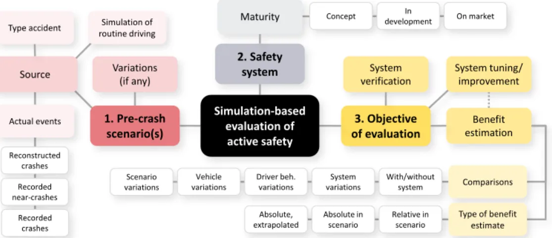
4 Simulation-based safety evaluation 33 4.1 Types of simulation-based evaluation . . . 33
4.2 A simulation-based evaluation of ESC . . . 35
4.3 Sketch of an AEBS what-if evaluation . . . 38
5 Frameworks for driver modeling 43 5.1 From routine driving to near-crash driving . . . 43
5.2 From sensorimotor heuristics to vehicle dynamics . . . 47
6 Conclusions and future work 49 6.1 The ESC and AEBS use cases . . . 49
6.2 Beyond the ESC and AEBS use cases . . . 51
6.3 Modeling frameworks . . . 53
Chapter 1
Introduction
A truck driver is taking her 30-ton vehicle down an arterial road, one which she knows well from almost daily passages during her fifteen years of professional experience. Traffic is flowing nicely, and there is just one more hour of work remaining before she can return home to her family. Suddenly, out of nowhere, our driver finds herself on a course for imminent, high-speed collision with the passenger car ahead, which is stopping for something, a traffic queue ahead, an animal passing on the road, or some obstacle blocking an intended exit from the road. Time freezes. The situation as such is clear, in all its minute detail: the distance separating truck and car, their current speeds and accelerations, how the two vehicles would respond to altered pedal or steering wheel inputs, the curvature of the road, the friction between asphalt and wheels. With all this knowledge, could we predict what will happen next? Will the truck driver crash into the rear of the passenger car, or will she brake quickly and strongly enough to stop behind it? Will she maybe reach the split-second decision to change lanes, and carry out a successful steering collision avoidance? Or will the specifics of her steering cause her to lose control over the truck, sending it skidding off the road? Crucially, what if the truck itself would have provided a warning to the driver, potentially making her realize the threat earlier? What if the truck would have applied automatic emergency braking as the collision drew nearer, or helped stabilize itself during skidding? Could such interventions have transformed a potentially fatal collision into nothing but a passing scare?
Any adult individual in modern society is well aware that road traffic occasionally leads to accidents, causing economic costs, injuries and sometimes even death. From a global or societal perspective, this is a major challenge. In 2010, 1.24 million people died in vehicle crashes [176], and current trends suggest that road traffic accidents will rise from being the ninth most common cause of death, worldwide, to a fifth place in 2030 [177]. Counting both fatalities and injuries, costs for crashes are estimated to amount to 1-3 % of countries’ gross domestic products [178].
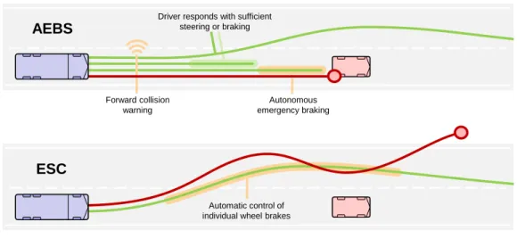
Furthermore, it is by now well established that driver behavior plays a major role in the causation of traffic accidents, in the form of for example inattention, excessive speeding, or inadequate evasive maneuvering [92, 156]. Based on such insights, recent accident prevention efforts by governments, industry, and academia, have placed a major emphasis on active safety technologies. These technologies provide warnings or control interventions with the aim of improving driver behavior or mitigating the effects of inadequate driver behavior, at the rare occurrences of a risk of, for example, vehicle instability, collision, or road departure [18, 68, 69]. Figure 1.1 introduces two active safety systems that will serve as recurring examples in this thesis: (i)advanced
Automatic control of individual wheel brakes
Autonomous emergency braking Forward collision
warning
Driver responds with sufficient steering or braking
AEBS
ESC
Figure 1.1: Illustration of how two active safety systems could prevent crashes (the red trajectories ending in circles) in a rear-end conflict scenario. Top: Advanced emergency braking system (AEBS), providing a forward collision warning (e.g. light and sound) to prompt a braking or steering response from the driver, and autonomous emergency braking when collision is imminent [78, 161]. Bottom: Electronic stability control (ESC), maintaining yaw stability of the truck in spite of limited road friction, by applying individual wheel brakes to achieve the trajectory indicated by the driver’s steering [153, 183].
emergency braking system (AEBS), with sub-functionalities forward collision
warning (FCW)andemergency brakeand (ii)electronic stability control (ESC).
As with any technology, active safety systems needevaluation, in order to determine to what extent they fulfill their intended purpose of reducing frequency or severity of crashes. System developers need to carry outformativeevaluation [98], in order to be able to optimize a system before making it available on the market, and governments, insurance agencies, and vehicle-buyers need summative evaluations [98] of the end-product, to know what it is worth, whether to subsidize it, or if it should perhaps even be made mandatory by law.
The high-level, societal perspective on accidents clearly motivates the efforts invested in active safety systems, but there is another perspective that one can also take, equally valid, but with some possibly serious implications for the evaluation of these systems:
From the perspective of the individual driver, accidents are extremely rare, and many
drivers never crash at all during their lifetime. In the U.S., a police-reported crash with person injury occurs only once every 3 million kilometers of driving, and the same figure for Sweden is once every 5 million kilometers [127]. In other words, even if driver behavior can be put to blame for most crashes, the average driver is nevertheless impressively proficient atnotcrashing. The question thus arises: How does one evaluate a system when its performance depends crucially on the interplay with human behavior in situations that, from a first-person perspective, practically never occur?
The research work reported in this thesis aims, in general, to address this challenge by 2
observing behavior in near-accident situations, and generalizing these observations into mathematical models of drivers’ near-accident control over their vehicles. Such driver models can provide quantitative answers to “what happens next?”types of questions, such as those formulated in the opening of this chapter, and can therefore permit evaluation of active safety systems in computer simulation [6, 20]. This approach has the potential to avoid some problems, related to cost or validity, of alternative evaluation methods. In order to maintain a manageable scope of behaviors to study and model, this thesis focuses on the two active safety systems shown in Figure 1.1, specifically in the depicted rear-end collision type of conflict scenario.
The remainder of this chapter provides introductions to the general state of knowledge with regards to driver behavior in accident situations, and existing methods for evaluation of active safety. Then, the main research questions and the general research approach are introduced, an outline is provided for the rest of the thesis, and the author’s contributions to the included papers are clarified.
1.1
Driver behavior and accident causation
How can one understand and describe behaviors such as, for example, those exhibited in Figure 1.1? On the conceptual level, there is a wealth of theories and models that propose different ways of how to best discuss driving, and sometimes also accidents [30, 34, 118, 151]. Here, a conceptual framework proposed by Ljung Aust and Engstr¨om [99], with the specific aim of supporting research in active safety, will be adopted.
In this framework, driving is viewed asadaptive behavior, the result of a balance betweenmotivationto fulfill high-level goals, such as reaching the destination on time, and feelings of discomfortexperienced in threatening situations. The driver and vehicle can together be regarded as a joint driver-vehicle system (JDVS) moving in the space of all possible states of the driver, vehicle, and the environment (aDVE state
space), and the extent to which the JDVS can control the trajectory in this space is
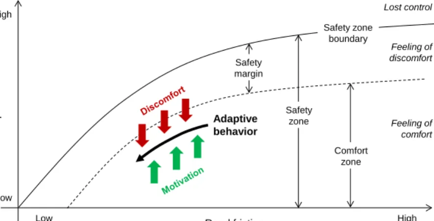
referred to as situational control. The region(s) in DVE space in which the driver does not experience any discomfort is called the comfort zone, and within this zone the driver is content with good-enough,satisficing [17, 146, 151] behavior. The comfort zone is typically entirely contained within thesafety zone, the region(s) of DVE state space outside which situational control is reduced to a degree where a crash is inevitable. Fig. 1.2 provides an illustration of these ideas in an example scenario where a driver perceives a drop in road friction, and adapts by reducing vehicle speed, to stay within the comfort zone and keep asafety marginto the safety zone boundary.
In the framework of Ljung Aust and Engstr¨om, accidents are described, in general, as loss of situational control due to the driver failing to adapt properly to a current or changing DVE state. Furthermore, the main mechanisms which may, alone or in combination, lead to such adaptation failures are suggested to be (i) erroneous perception of the current safety zone boundary, (ii) overestimation of one’s own ability, or that of the vehicle, (iii) an incorrect prediction of how a situation will develop over time, and (iv) rapidly occurring, unexpected events. Finally, the role of active safety systems is to help the driver adapt to DVE state changes, in order to ensure that situational control is
Safety zone Comfort zone Safety margin Safety zone boundary Feeling of discomfort Lost control Feeling of comfort Adaptive behavior High Low S peed High Low Road friction
Figure 1.2: Illustrations of key concepts of the conceptual framework of Ljung Aust and Engstr¨om, in a hypothetical scenario where a driver perceives a drop in road friction, and thus reduces vehicle speed to avoid experiencing feelings of discomfort. After [99].
maintained.
This type of general framework is needed to structure thinking and writing. However, if one wants a more detailed description of driver behavior, for example to run computer simulations, there is a range of additional questions that require very specific answers. What information on the current DVE state do drivers perceive and use when controlling their trajectory in DVE state space? How do they translate these sensory inputs to control actions, and how can this process be described mathematically? Another phenomenon that cannot be neglected at this level isbehavioral variability, i.e. variations in behavior either between drivers, due to factors such as driving experience [25, 37, 86] or personality [154], or within a given driver depending on factors such as for example fatigue [4] or effort [31, 64].
There exists a wide range of detailed, simulation-ready models, providing different answers to the questions listed above, and some of these models also account to some degree for behavioral variability [61, 63, 131]. However, these models typically address routine driving, leaving one potential source of within-driver variability, highly relevant to this thesis, largely unexplored: the shift from routine driving to more critical situations. Here, driver behavior that occurs close to a possible crash will be referred to as
near-crash behavior, typically characterized as different from routine driver behavior in a
number of ways. For example, near-crashing drivers often exhibit very slow reactions, or no reactions at all, even to stimuli that would seem to motivate immediate reactions [60, 94, 170]. Furthermore, when reactions come, they may (in hindsight) seem improperly chosen, such as braking and colliding when a steering maneuver could have avoided the crash [3, 90], or may come in the form of overreactions [105, 175] or underreactions not utilizing the full performance capabilities of the vehicle [3, 81, 90]. Some of the main candidates for factors explaining such phenomena include a limited driverexpectancy
of the threatening situation, emotionalarousal, as in fear or panic, a highuncertainty
of how other road users will behave, and drivers having a very limitedexperienceof severe maneuvering [19, 28, 60, 90].
Does this mean that models of near-crash behavior ought to be fundamentally different from non-emergency models? If yes, must evaluation of active safety systems consider not only behavioral variability in general, but also specficially factors such as expectancy, fear, uncertainty, and inexperience?
1.2
Evaluation of active safety functions
Arguably, the only way of evaluating active safety that is completely valid, from a driver behavior perspective, is to exclusively considernaturalisticsituations, as in real critical situations, in real traffic. The most straightforward approach to doing so is to use statistics from e.g. accident databases or insurance claims records: After market introduction of a safety system, one may simply wait for a sufficient number of accidents to occur, and then investigate whether system-equipped vehicles are involved in fewer or less severe crashes than other vehicles. From passenger car statistics, ESC has been shown to prevent about 40 % of all crashes involving loss of control [67], and AEBS has been found to reduce property damage insurance claims by 10-14 % [68].
A related approach, yielding more rich data sets, thus allowing deeper insights into system-related driver behavior, is to conductfield operational tests (FOTs), in which logging equipment is installed in fleets of vehicles, operated by regular drivers during extended periods of time. The author is not aware of any FOTs targeting ESC, but both for passenger cars and trucks, FOTs have demonstrated benefits of the FCW component of AEBS, in terms of faster reactions to conflicts [8] or fewer harsh braking incidents [74]. One clear limitation with this type of approach is the high cost. In addition, a necessary limitation of any naturalistic evaluation method is the requirement of having system hardware and software mature enough for prolonged use by end-users. In practice, this means that naturalistic evaluation will be more summative than formative in character. In order to perform formative evaluation, system developers often turn totest tracks, where early prototypes can be subjected to controlled testing. For ESC, this type of evaluation generally has an experienced test driver follow a predefined path, or a driving robot carry out predetermined steering maneuvers inopen-loop fashion [97, 158], as opposed toclosed-loopmaneuvering, where the outcome of past control is continuously taken into account to update later control. For AEBS, the vehicle under evaluation is typically set on a collision course with a moving or static obstacle, and sometimes a driver response to FCW is emulated by a driving robot applying open-loop braking [5, 7, 39]. An important benefit of evaluating on the test track is the relatively high
repeatability, allowing efficient comparison of the outcome with and without a system,
between alternative versions of a system, or between different makes and models of system-equipped vehicles. Consequently, this is also the approach used for type approval and safety rating of on-market ESC and AEBS [38–40, 158].
However, it should be acknowledged that much realism in driver behavior may have been sacrificed in order to reach this repeatability. It seems likely that driving robots executing predetermined pedal or steering wheel movements, or experienced test drivers
following cone tracks, produce a much less varied range of behaviors than normal drivers in near-crash situations. In some cases, it could even remain to be proven that the specific range of behaviors studied on the test track is at all represented in real traffic. This is not to say that active safety systems evaluated on the test track do not provide real benefits for traffic safety (as mentioned above, accident statistics show that they do), but it could for example mean that a better performance of system A than system B in a test track evaluation does not guarantee that system A will provide the greater benefit in reality.
One means of obtaining more realistic driver behavior is to try to stage unexpected events on a test track [42, 78]. Another is to usedriving simulators. In simulators, a sample from a population of normal drivers can be safely subjected to near-crash scenarios that are, if not entirely unexpected and realistic, at least more so than typical test track scenarios. Especially FCW has been extensively researched in this way, from a large number of different perspectives [2, 27, 93, 96, 100, 116], but also the emergency braking component of AEBS [120], as well as ESC [26, 115, 130].
In general, these simulator studies have been able to demonstrate beneficial safety effects of the tested systems, even under the increased variability in behaviors exhibited by surprised drivers. However, the higher experimental validity comes at a price: In order to maintain sufficient statistical power despite behavioral variability, simulator studies typically have to address a more limited range of experimental conditions (e.g. number of traffic scenario variations, number of system variations, etc.) than test track studies, and need a larger number of measurements per condition. Furthermore, driver expectancies for critical situations typically increase with exposure, making it difficult to validly record near-crash behavior more than once per subject [32]. In sum, cost is definitely a concern also for simulator-based system evaluation.
Possibly the most cost-efficient evaluation method of all, then, would be to exclude the human drivers altogether, and replace them withmathematical models of human
behavior. Using driver behavior models, relevant scenarios can be simulated with even
greater repeatability than on the test track, as many times as wanted. Table 1.1 provides a summary comparison of the various evaluation methods introduced in this section.
At the outset of the research project behind this thesis, ESC had been subjected to evaluation in computer simulation, but only as simulated reproductions of test track evaluations [75, 87, 153, 169]. Active safety evaluations that are instead based on more realistic near-crash simulations have started to become available mainly in the last five years [6, 29, 36, 51, 83, 84, 119, 126, 142, 173, 174], although some earlier examples exist, mainly concerning FCW [20, 45, 93, 150]. One important milestone in this area was the National Highway Traffic Safety Administration (NHTSA) Advanced Crash Avoidance Technologies (ACAT) program, with the first projects ending around 2010; a main target for ACAT was to develop a U.S. national level benefits estimation methodology, with simulation as a key component [22, 48]. Indeed, as ever growing quantities of actual logged, time-course data from accidents are becoming available, from large-scale naturalistic studies [159] or widely deployed systems for monitoring or event recording [35, 85],what-if resimulation, where one estimates what impact an active safety system would have had on a set of actual crashes, seems like a very attractive approach for active safety evaluation.
More will be said about these existing approaches to simulation-based evaluation 6
Table 1.1: Comparison of alternative methods for evaluating active safety systems. The main purpose is to highlight differences between methods; specific evaluations may depart significantly from the typical characterizations provided here.
System evaluation method
Combinations of system and scenario variations Approximate cost, nearest power of 10 Development phase Realism of driver behavior Analysis of existing accident data (featur-ing the system)
One system alterna-tive; no experimental control over scenarios
≈10 ke Summative Full
Field operational test -”- ≈1 000 ke Mainly summa-tive
Full
Test track evaluation ≈10 ≈10 ke Formative and summative
Low
Driving simulator ex-periment
≈4 ≈100 ke -”- High
Computer simulation >1 000 ≈10 ke* -”- Depends on the driver model * Assuming that no major effort is needed to develop e.g. driver models, traffic scenarios to simulate, etc.
later in this thesis. For now, what about the driver models? After all, as pointed out in Table 1.1, the realism of a simulation is limited by the realism of its models. In the previous simulation-based evaluations of FCW and AEBS cited above, the driver model has recurrently been of the simple, open-loop type that could easily be implemented in a driving robot, e.g. applying a constant decelerationda reaction timeTRafter warning, two parameters which may be either fixed or drawn from probability distributions. Is this type of model close enough to reality to produce acceptably correct evaluation results? For example, several studies have noted that FCW may redirect a driver’s off-road eye gaze back to the road, but the actual control responses seem to come rather in response to the rear-end situation than to the warning itself [93, 100, 167]. This could point to a need for more situation-dependent driver models. In the previous simulations of ESC in realistic near-crash scenarios, there is one example of what seems to be open-loop modeling [29] and one example of closed-loop modeling [119], however in the latter case using a model which does not seem to have been validated on near-crash behavior data [95]. Again, do these models capture enough of what human drivers do in real critical situations for the evaluations to be of any value? Such questions are at the very core of what is being addressed in this thesis.
1.3
Research objectives and thesis structure
As previously mentioned, the general aim of the present research work has been to identify models that accurately describe near-crash driver behavior, in order to ensure validity of simulation-based active safety evaluations.
However, rather than aiming for models that would be applicable across many different traffic scenarios and active safety systems, modeling has been constrained to two specific
use cases for driver-vehicle-environment (DVE) simulation. These were chosen by considering both the applied relevance for the involved industrial project partners, and the estimated potential for making a valuable scientific contribution to driver modeling.
In the ESC use case, driver models and simulations have been developed to answer
the following research questions:
(A) Does heavy truck ESC provide a safety benefit for normal drivers in
realistic near-crash maneuvering? Accident statistics provide strong evidence
for the safety benefit of passenger car ESC [67], but similar investigations have not been possible yet for trucks, because of limited market penetration [175]. Also in simulator studies, benefits of passenger car ESC have been proven [115, 130], but the only similar study on trucks was unable to find a statistically significant effect, possibly due to a too small sample size [26].
(B) Is ESC equally useful for all drivers in realistic near-crash maneuvering?
A potential advantage of driver modeling is the possibility of isolating and studying behavior of individual drivers [37, 182], for example to understand whether ESC should work differently for different drivers. This research question was further motivated by anecdotal reports of ESC sometimes being perceived to interfere with routine driving; could indications of such interference be found in critical situations?
Inthe AEBS use case, the target has been to develop driver models and simulations for
what-if evaluation of heavy truck AEBS on actual logged time-course data from rear-end crashes. In other words, the main research question has been:
(C) For a given recorded rear-end crash, what would have happened if AEBS
had been present? A full answer to this question requires both a methodology
for what-if evaluation and good models of many aspects of driver behavior, and this thesis will only partially address these needs. A sketch of an evaluation method will be provided, and one specific model-related question will be explored in some detail:
(D) Is the timing of drivers’ defensive maneuvers in rear-end conflicts de-pendent on the specific situation kinematics, and, if so, how can this
dependence be modeled? As mentioned above, existing simulation-based
evalu-ations of AEBS-like systems have posited kinematics-independent distributions, but several studies suggest that this is an insufficient account of driver behavior. A three-step approach, also reflected in the structure of this thesis, has been adopted for both use cases:
1. Measure human control behaviorin as relevant and realistic settings as possible
(Chapter 2). This has involved one simulator experiment on ESC, and analysis of one naturalistic data set on rear-end crashes and near-crashes.
2. Identify driver modelsthat can reproduce the observed control behavior
(Chap-ter 3). Answering research question D is an obvious aim of this part of the process, but as we shall see, it is possible already at this stage to answer also question A.
3. Implement and run simulations that are required by the use cases (Chapter 4). This includes providing an answer to research question B, as well as a sketch of the envisioned approach for answering research question C.
Each of the Chapters 2 through 4 will first address the topic at hand from a general perspective, before presenting the specific efforts made in relation to the two use cases.
Finally, a secondary research aim has been to evaluate the possibility of generalizing the very delimited, use case-specific driver models into a more general modeling framework. This will be the topic of Chapter 5. Finally, in Chapter 6, conclusions will be made, and an outlook towards the future will be provided.
1.4
Contributions to the included papers
The author had the main responsibility for designing the ESC simulator study, providing the data set for Papers I, II, and V. The author also carried out the statistical analyses for Paper I, and wrote most of the text. For Paper II, the author collaborated with Benderius in determining the analysis approach, and assisted in the writing. The author collaborated with Victor, B¨argman, Engstr¨om, and Boda in extracting the data set and determining the analysis approach for Paper III, but did the analysis and writing himself. Preparations for and writing of the review in Paper IV was done in collaboration with Benderius, Wolff, and Wahde. The author generated the model-fitting results and analyses presented in Paper V, and wrote the paper. Paper VI was the author’s product in its entirety.
Chapter 2
Measuring near-crash behavior
In the previous chapter, the main empirical approaches to human-in-the-loop evaluation of active safety were listed: naturalistic driving studies and controlled studies on test tracks or in simulators. These same approaches are useful also when collecting data for driver models, with the same considerations in terms of cost and driver behavior realism (Table 1.1). However, on closer inspection, the specific objective of supporting driver modeling, rather than evaluating a safety system, implies specific constraints for experimental design. The first section of this chapter will take a closer look at the concept of behavioral variability, to discuss how such variability is the very foundation for useful modeling while at the same time creating serious challenges for useful data collection. The remainder of the chapter will present the two specific data collection efforts covered in this thesis, together with results from initial, statistical analyses of the obtained data.
2.1
Aspects of behavioral variability
Human behavior is enormously variable, affected in myriad ways both by the state of the external world, observable to a third-party experimenter, and the internal states of the body and the brain, generally hidden from observation. Consider, again, the example rear-end situation sketched at the start of the previous chapter, and assume that one describes this specific DVE state, in detail, in the form of a very long vectorXΩof DVE parameters. Now, if one could twice very closely replicate the same traffic situationXΩ, why not even down to the state of individual neurons in the truck driver’s brain, one would expect that the truck driver would twice exhibit very similar control responses, pedal and steering wheel actions described in a vectorY. If specific individual DVE parameters inXΩ were varied gradually, variations in Y would be expected. These variations in behavior could also be gradual, such as schematically illustrated in Fig. 2.1a, but there could just as well be more dramatic effects, for instance a small change in a headway distance causing a transition from a steering response to a braking response.
Driver modeling, as it is addressed in this thesis, amounts to finding mathematical expressions that describe relevant aspects of behavioral variability, in the form of mappings toY from some subsetX={X1, X2, ...}of the DVE parameters inXΩ. Consequently, experiments aiming to provide data for modeling should measureY while, ideally, varying all of the DVE parameters inX independently. This ideal is not easy to live up to, but even if one can, there will now always be behavioral variability that the model can never account for, due to the dramatic simplification of passing from XΩ to X. Fig. 2.1b illustrates this effect by showing a random sampling of the range of situations depicted in
X 2 DVE parameter X 1 Driver behavior Y (a) DVE parameter X 1 Driver behavior Y (b) DVE parameter X 1 Driver behavior Y (c)
Figure 2.1: Schematic illustrations of (a) a hypothetical effect of two Driver-Vehicle-Environment (DVE) parameters on a driver behavior variable Y, (b) behavioral variability from an uncontrolled DVE parameter, and (c) behavioral variability between different drivers (the four different curves), within each driver (the shaded areas around the curves), and one measurement from each driver (the rings) at one of two values ofX1.
Fig. 2.1a, but without measuringX2. In the rear-end collision example,X1could betime
to collision(TTC, relative distance divided by relative speed),X2some quantification
of how unexpected the rear-end conflict is to the truck driver, andY could be the time until the truck driver starts braking. In a naturalistic setting, one may measure X1, but will most probably have very vague notions, if any, ofX2. The variations in this
uncontrolled parametershow up in Fig. 2.1b as behavioral variability, making the
relationship betweenX1 andY more imprecise and difficult to discern.
Variability from uncontrolled parameters is the reason why non-naturalistic experiments on human behavior typically attempt to put all subjects in the exact same circumstances; if all drivers in a simulator study have had the same experiences from the start up until a sudden lead vehicle deceleration, chances are greater that X2 in our example will be similar between measurements. However, even with perfect experimental control of this kind, other uncontrolled parameters related to the individual drivers will remain:
Between-subject variationsin some parameters will cause the mapping from X1 to
Y to differ between subjects, as exemplified by the four different curves in Fig. 2.1c. The shaded areas around these curves intend to illustrate howwithin-subject variations
will also always arise, even if it is possible to sample the sameX1→Y mapping several times. Furthermore, if the mapping is affected by some uncontrolled parameter that is influenced by measurement itself, such as the expectancy-relatedX2 above, one may only be able to record once from each subject before behavior adapts and the mapping changes. In cases where the only aim is to demonstrate thatX1has some kind of impact onY, the typical approach, illustrated by the rings in Fig. 2.1c, is to sample each driver at one of two distinct values ofX1, and test for a statistically significant difference. However, if the relationship betweenX1 andY must be described more completely in a driver model, a better coverage ofX1 is required. Additionally, if the aim is to elucidate between-driver differences in theX1→Y mapping, such as in the ESC use case considered in this thesis, one needs this coverage ofX1 also for each individual driver. How can this be achieved?
2.2
A simulator study on near-crash steering
In the ESC use case, the primary target for modeling was driver steering in the low-friction, rear-end type of scenario illustrated in the bottom panel of Fig. 1.1, where the driver first steers away from an impending collision and then stabilizes the vehicle on the road1. In other words, in each time step of an envisioned computer simulation, the driver
model should be able to predict steering behaviorY as a function of a vectorX of DVE parameters, for example regarding vehicle positions and speeds on the road, angles or rates of change of vehicleyaw(horizontal orientation), etc. Thus, here, a single recorded scenario of human steering passes through many DVE statesX, and therefore provides many measured pairs ofX andY. However, sinceX is now multidimensional, a single scenario will still only provide a rather limited view of the completeX→Y mapping.
To gather enough data for a study of steering on the level of individual drivers, a 24-subject driving simulator study was designed, with two distinct stages. First, each driver was exposed, once, to a rear-end conflict scenario that was intended to be as unexpected as possible; a higher-speed lead vehicle overtaking the truck and continuing ahead for a while, before suddenly decelerating for no apparent reason [33]. Next, a novel experimental paradigm ensued, where repetitions of the same critical scenario were randomly interleaved withcatch trials. In the catch trials, the lead vehicle decelerated only for a short while, such that braking alone was enough to avoid collision. By careful design of the exact scenario parameters, and by instructing the drivers only to perform steering avoidance when they deemed that this was necessary, repeated avoidance steering from a low TTC of between 2 and 3 seconds could be observed. As shown in Fig. 2.2, this was the most common point of avoidance steering also in the unexpected scenario. Crucially, this was a point from which collision avoidance and stabilization was challenging given the low road friction (µ= 0.25), prompting frequent engagement of the ESC system, a software-in-the-loop implementation of an actual on-market system from Volvo Trucks. Full details on the simulator experiment are available in Paper I, and further insight into the process for arriving at the final experiment design is provided in the author’s licentiate thesis [106].
In order to get some experimental control over individual differences, drivers were recruited into two groups: One low-experience group of drivers who had just obtained, or were just about to obtain, their truck driving licenses, and one high-experience group, with at least six years of professional truck driving experience. In the unexpected scenario, these groups differed markedly with respect to reaction times. While drivers in both groups typically followed the pattern of first braking, and then, in a majority of cases, also applying avoidance steering, the experienced drivers both braked and steered significantly earlier than the novice drivers, and the novice drivers collided significantly more often.
Fig. 2.3a shows the difference in steering reaction times, while also making another important point: Both the observed steering reaction times and the percentages of drivers who at all applied evasive steering (70 % and 82 %, in the low and high experience groups, respectively) could be explained by the same reaction time distributions. In existing
1This specific scenario was chosen both because it was deemed well-suited for simulation-based
evaluation, and because avoidance maneuvers are known to be an important cause of heavy truck yaw instability [75]; a more detailed argument can be found in the author’s licentiate thesis [106].
100 50 0 50 100 150 200 0 2 4 6 8 Longitudinal position (m) Lateral position (m) 100 50 0 50 100 150 200 0 2 4 6 8 Longitudinal position (m) Lateral position (m) 0 1 2 3 4 5 6 7 8 9 10 0 30 60 Frequency(%) Repeated avoidance TTC at steering initiation (s) 0 1 2 3 4 5 6 7 8 9 10 0 30 60 Frequency(%) Unexpected avoidance TTC at steering initiation (s)
Figure 2.2: Steering in the unexpected (top panels) and repeated (bottom panels) scenarios of the ESC simulator study. The panels on the left show the recorded truck trajectories, and the panels on the right show the distributions of time left to collision with the lead vehicle, when truck driver steering first exceeded15◦. Longitudinal position zero corresponds to the point at which the truck’s front reached the rear of the lead vehicle. From Paper I.
(a) 0 1 2 3 4 5 6 7 0 20 40 60 80 100 70% 82%
Steering reaction time (s)
Cumulative frequency (%)
Low exp. data Low exp. fit High exp. data High exp. fit Time of coll. (b) Low High 0 5 10 15 20 Experience
Max. body slip angle (deg)
ESC state Off On
Figure 2.3: (a) Cumulative steering reaction times after lead vehicle brake light onset in the unexpected scenario, up to the observed proportions of drivers applying steering, with least-squares fit of distributions (log-normal, as is often found suitable for reaction times [157]). The shaded region shows the time range within which all collisions occurred. (b) Effect of ESC on skidding, in the repeated scenario. Both panels from Paper I.
models of driver behavior in rear-end conflicts, fixed probabilities have typically been adopted for the various basic avoidance maneuvers, e.g. “braking only” versus “braking and steering”[6, 150]. Fig. 2.3a instead suggests that reaction time distributions might be a more appropriate level of modeling, with probabilities of non-reaction arising naturally from reactions sometimes being too slow given the kinematics of the specific situation.
With regards to the ESC system, no significant effects of its presence were observed in the unexpected scenario. However, in the repeated scenario, ESC significantly reduced maximumbody slip angle(Fig. 2.3b), i.e. how much the vehicle’s front points away from the current movement direction, and frequency of full control loss, i.e. road departures and spin-arounds. One possible explanation for this difference in ESC impact is that there was simply not enough ESC-relevant data in the unexpected case. Indeed, there were only nine recordings of the unexpected scenario where steering was vigorous enough to potentially elicit ESC interventions, versus 217 such recordings of the repeated scenario. On the other hand, there is also the possibility that the drivers substantially changed their steering behavior (theX→Y mapping) between the two scenarios, and that the steering behavior in the unexpected scenario, presumably more realistic, was somehow less compatible with the ESC system. This possibility needs to be carefully considered, since the very idea behind the design of this experiment was that near-crash steering behavior might be reasonably conserved between unexpected and repeated measurement, such that driver models developed based on the repeated measurements might come reasonably close to behavior in realistic, unexpected scenarios.
Therefore, as reported in Paper II, statistical comparisons were carried out regarding steering behavior in the two scenarios, for a subset of eight drivers where such comparison was considered feasible, and for those parts of the scenario where suitable quantitative metrics could be readily defined. During collision avoidance and initial alignment with the left lane (see Fig. 2.4a), no statistically significant effects were found of scenario or repetition, on maximum angles or rates of steering (see example in Fig. 2.4b), or on
steering wheel reversal rate, i.e. the frequency of small steering corrections [114]. For
maximum angles and rates, traces of such behavior conservation were discernible also at the level of individual drivers; as shown in Fig. 2.4c, the two drivers who steered very fast during lane alignment in the unexpected scenario, did so also in the repeated scenario. However, this type of correlation between unexpected and repeated scenario behavior was not observed for the reversal rates (Fig. 2.4d). These were generally lower in repeated than in unexpected steering, consistent with previous proposals of increased experience and expectancy leading to steering that is more smooth and open-loop in character [37, 66].
In sum, the statistical analyses of the collected data allow the conclusions that ESC provided a benefit in the repeated scenario, and that there were more similarities than differences between unexpected and repeated steering, in the initial phases of collision avoidance and lane alignment. This goes some way towards suggesting that the ESC system should be helpful also in unexpected situations (research question A of this thesis), but the argument is weakened by the limited number of drivers considered in the behavior comparison, and the exclusion from comparison of the final stabilization phase of steering, more difficult to characterize with scalar metrics. With regards to individual differences in ESC benefit (research question B), the positive effect of ESC was potentially slightly
time steer ing w h ee l ang le I3 I4 t0 t2 t3 t4 I1 I2 t1 (a) 0 50 100 150 200 250 UA RA st. wh. angle t 4 ( ° ) 0 50 100 150 200 250 RA 1−6 (b) (c) (d)
Figure 2.4: (a) Phases of typical steering in the ESC study, with I3 being collision avoidance, andI4 alignment with the new lane. (b) Comparison of steering wheel angle at t4, between unexpected and repeated avoidance (UA and RA), as well as over repetitions (RA 1-6). (c and d) Individual steering behavior, conserved between scenarios for steering wheel rate in segmentI4 (panel c), but not for steering wheel reversal rate inI3 (panel d). All panels from Paper II.
smaller for experienced drivers. When analyzing the two groups separately, the effect of ESC on full control loss did remain significant for both groups, but the effect on maximum body slip (Fig. 2.3b) was significant only for the novices. However, this type of group-level conclusion is still a far cry from saying anything meaningful about ESC in relation to
individuals. These issues will be explored further in the coming chapters.
2.3
Near-crash response timing in naturalistic data
During the years 2011-2013, the world’s largest naturalistic driving study to date was carried out in the U.S., as part of thesecond Strategic Highway Research Program
(SHRP 2). In this study, logging equipment was installed in the vehicles of more than
3000 volunteering drivers, generating a total of almost 80 million kilometers, or more than a hundred around-the-clock person-years, of recorded driving [15]. Paper III is an excerpt from the final report [159] of one of the associated analysis projects, dealing specifically with rear-end crashes and their relation to driver inattention, such asvisual distraction
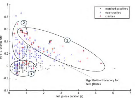
Figure 2.5: Categorization of rear-end conflicts by duration of final off-road glance and average rate of change of inverse time to collision (TTC) during the glance. From [159]; note that this analysis is not part of the excerpt, from the same report, in Paper III.
in the form of driver glances off the forward roadway. In this project, 46 rear-end crashes and 211 near-crashes were identified in the SHRP 2 data, both by means of automatic detection using various criteria, and other means such as incident reports from the drivers.
One important outcome of analyzing these events was a categorization of rear-end crashes, shown in Fig. 2.5, in terms of the interplay between visual distraction and the rear-end conflict itself. To interpret this figure, consider first the concept of inverse TTC
(invTTC = 1/TTC). As a crash draws nearer, TTC decreases, and therefore invTTC increases, an increase which is faster closer to a crash, and faster for higher lead vehicle deceleration rates. In this sense, invTTC change rate is a measure of the kinematic severity of the rear-end conflict. Another reason for considering invTTC as a quantity is that it is plausibly available to the collision-avoiding human driver: For a givenoptical
angleθof an obstacle on the driver’s retina, with time derivative ˙θ, known as theoptical
expansionorlooming, it is a well-known result [91] that TTC≈τ≡θ/θ˙, and 1/τ = ˙θ/θ
thus provides a visual estimate of invTTC2. It is also well established that there are
dedicated neural circuits for looming detection in animal brains, implicated in for example collision-avoiding behaviors [46, 152]. Probable homologues of these looming-detection circuits have been identified in the human brain [14].
2It may be noted that ˙θ/θalso has a direct interpretation in terms of therelativerate of expansion on
the retina. For example, if an obstacle grows on one’s retina by a third of its original size in 1 second, one knows that 1/TTC≈1/3, i.e. that a collision is 3 seconds away, regardless of other factors such as approach speed, distance, and object size.
Returning to Fig. 2.5, a majority of the extracted SHRP 2 crashes, labeled as Category 1, can now be understood as a perfect mismatch between glance duration and the nature of a rear-end conflict that arose during the glance: Very long off-road glances can cause crashes even in situations that are kinematically rather benign (low invTTC change rate), whereas in high-severity kinematics (high invTTC change rate), even very short glances might contribute to a crash. Category 2 crashes were found to be cases where the drivers glanced away briefly from an already established conflict, often in circumstances with reduced visibility. Category 3 crashes, finally, were cases where the conflict aroseafter
the final glance, such that the glance itself may have been less involved in the causation of the crash.
In relation to research questions C and D of this thesis, the analysis presented in Paper III aimed to clarify what happenedafter the final off-road glance. Specifically, the timing of a manually annotatedphysical reaction point, defined as “the first visible reaction [of the driver to the lead vehicle, such as a] body movement, a change in facial expression etc.”, was studied, as a proxy for timing of evasive braking or steering responses. Arguably, it would have been better to identify the onset of these maneuvers directly, but this was found to be difficult, partially because of limitations in data availability and quality. Furthermore, a well-defined onset may not always be present (see further Sect. 5.1). Reassuringly, however, follow-up analyses, not presented in Paper III or [159], have shown that peak decelerations were almost without exception reached after the physical reaction point, and in a majority of cases less than 0.5 s after it.
Even if the exact meaning and usefulness of the physical reaction point can be discussed, with the SHRP 2 data set there can be no questioning the validity of the observed behavior as such. This is a welcome contrast to the ESC study, where major efforts have been required for understanding the validity of the repeated-scenario behavior. However, as will become clear in the next chapter, the SHRP 2 data have other limitations, for example related to the issue of uncontrolled parameters, as introduced in Sect. 2.1, and to whether or not the selection of what events to include introduces biases in the data.
To summarize, there is probably no single perfect approach to measuring near-crash behavior. Controlled studies allow isolation of individual behavioral phenomena and mechanisms, and can therefore be highly useful in the development of models, whereas naturalistic data, unstructured but with full validity, provide the ultimate benchmark for model refutation or corroboration.
Chapter 3
Models of near-crash behavior
In its most general sense, amodelin science is just “a simplified description of a system or process”[129], a very broad notion indeed. Consequently, the termdriver model can be understood to mean a number of different things, for instance aconceptual model
of driver behavior, like the framework by Ljung Aust and Engstr¨om outlined in Chapter 1. As clarified in Chapter 2, models to be used in evaluation of active safety typically need to be more quantitative in nature, mapping DVE states to mathematical descriptions of driver control behavior. This mapping can take the form of astatistical model, for example providing probability distributions for some limited aspect of control behavior, such as reaction times, in one or more DVE states. For full applicability, models should be able to close the control loop needed for computer simulation, by specifying momentary control actions as a function of momentary or previous DVE states, as was sketched for the ESC use case in Sect. 2.2. Models meeting this requirement can be referred to as
process models[141] of driving behavior.
There is a wealth of alternative approaches to such process modeling, and the first section of this chapter provides a brief inventory. The three remaining sections describe (i) a comparison of candidate process models for the ESC use case, (ii) how a few of these were used to further clarify the ESC simulator study’s validity, and (iii) a model of response timing in situations with risk of rear-end collision, such as observed in SHRP 2.
3.1
Understanding the alternatives
At the outset of this research project, it was clear that many process models of driving control behavior had already been proposed (see e.g. [131]), but it was less clear how much of this previous work had targeted behavior in more critical situations. Therefore, an extensive literature search was carried out, considering more than 5000 literature database search hits from the years 2000 to 2010. The result was a collection of more than 60 identified instances of near-crash behavior simulation, reviewed in Paper IV. Most of these previous simulation efforts also proposed their own specific driver models (in many cases this was the main research objective), either completely novel or as modifications of existing models. However, some recurring themes in modeling could be discerned.
A common type of very simple driver model, alluded to already in Chapter 1, could be referred to as adelayed open-loop maneuvermodel: A reaction timeTRafter some event, e.g. a brake light onset or a driver glance back to the road, the driver applies a rapid braking or steering maneuverM, without closed-loop control. Variants of such a model, withTRandM for example drawn from fixed probability distributions, have been
Desired path Optical lever
(a)Sharpet al. [143]
Desired path Computed optimal path (b)MacAdam [101] Current path Required path Boundary points X4
(c)Gordon & Magnuski [59]
Target lat. pos.
Near point Far point
X3 (d)Salvucci & Gray [140]
Figure 3.1: Schematic illustrations of four models of steering from the literature. Specific implementation details can be found in Paper V.
used not least in what-if resimulations of accidents [45, 150], also in more recent work, published after Paper IV was written [6, 83, 84, 126].
The delayed open-loop maneuver type of model clearly attempts to capture a specific near-crash type of behavior. Other researchers have instead adopted models or modeling paradigms from routine driving, applying them in near-crash simulation. Fig. 3.1 illustrates four examples of this approach, roughly representing four different types of model. The Sharpet al. [143] model in Fig. 3.1a is an example of a model inspired bycontrol theory. Since the dawn of driver modeling, researchers with a good insight into the theory of automatic control of machines have likened the human driver to such controllers [71, 168]. Pedal or steering wheel control has thus been modeled as a function of a set of control
errorsto be minimized. In the Sharp et al. model, steering wheel angleδis applied as:
δ=Kψeψ+K1e1+Kp
n
X
i=2
Kiei (3.1)
aiming to minimize the heading and lateral position deviationseψ andei from adesired
path, as schematically illustrated in Fig. 3.1a. TheKarecontrol gains. In longitudinal
car-following, typical control errors to minimize have been deviations from zero relative
speed [50] or from a desired time headway [181]. Aneuromuscular delayon the order of 0.2 s is often introduced between input and output.
As control theory has become more advanced, so have the driver models derived from it.
Inoptimal control theory, the aim is to apply a control that is, in some sense, optimal.
For example, the driver model by MacAdam [101], illustrated in Fig. 3.1b, applies the steering angle that minimizes an integral of predicted lateral deviation from the desired path. To achieve this prediction, the driver model relies on aninternal vehicle model1,
1In MacAdam’s [101] model, this is alinear one-track model; see Paper V for a full formulation.
considered to operationalize the driver’s acquired understanding of vehicle dynamics. An added practical benefit is that the same driver model may easily be reused together with many different simulated vehicles, accounting for behavioral adaptation to changing vehicle dynamics [103] by simply updating the internal vehicle model.
Other optimal control models have utilized more advanced, compound optimality criteria, for example to manage both longitudinal and lateral control at the same time, or to trade control accuracy against driver effort [21, 132]. The latter optimization trade-off is one way of accounting for the phenomenon of satisficing (introduced in Sect. 1.1), obvious especially in routine driving circumstances. The model by Gordon & Magnuski [59], illustrated in Fig. 3.1c and applied to collision avoidance in [23], also includes a basic internal vehicle model, but achieves satisficing more directly, by only applying steering corrections if the vehicle’s current path violates a set of boundary points, representing edges of lanes or collision obstacles. The car-following model by Gipps [52] applies satisficing longitudinal control in a related fashion, and elaborated versions of this model have been applied in simulation of near-crash situations [62, 179].
All of the models presented above have taken a predominantly engineering-oriented perspective on driving, by emphasizing control and vehicle dynamics. Meanwhile, more psychology-oriented researchers have emphasized the question of what specific sources of perceptually available information, often referred to asperceptual cues, are used in driving control. For steering, it has been shown that limited visual information from one region close to the vehicle and one region further down the road is enough to reach the same performance as with a full visual field [89]. Consequently, the model by Salvucci & Gray [140], Fig. 3.1d, uses only the visual anglesθn andθf to one near pointand one
far pointfor steering the vehicle towards a target lateral position:
˙
δ=knPθn˙ +kfθf˙ +knIθn (3.2)
Here, dots over quantities denote differentiation with respect to time. In other words, the Salvucci & Gray model starts rotating the steering wheel as soon as either the near point or the far point starts to move, or if the near point is not centered in front of the vehicle. It may be noted that Eq. (3.2) is rather similar in form to Eq. (3.1); the main difference lies in the choice of psychologically plausible perceptual cues as control errors, and the control of steering wheel rate ˙δrather than steering wheel angleδ, inspired by [166]. Salvucci and colleagues [137, 139] have also integrated this steering control model into a more completecognitive architecture, to allow simulation of a wider range of driver behavior, including execution of visually distracting secondary tasks [138].
While the review in Paper IV found many instances of near-crash behavior simulation, based on the abovementioned driver models and others, two clear research gaps were also noted. First, novel driver models had generally been proposed without comparing them to existing, competing models, leaving it unclear how similar or different the predicted behavior would actually be. Second, almost none of the proposed models had been validated on human behavior data from real or realistic near-crash situations. The main exception was the successful fitting of a Gipps-like longitudinal control model by Xin
et al., to a small set of actual recorded queue crashes [179]. In the cases where steering models like those shown in Fig. 3.1 had been tested against human steering, this was in the cone track type of scenarios described in Sect. 1.2, with questionable external validity.
3.2
A comparison of steering models
In order to improve the understanding of how various near-crash behavior models relate to each other, the review in Paper IV provided limited simulation-based comparisons of a few braking and steering models, indicating that predicted behavior may sometimes be more similar than what can be readily deduced from the model equations. However, in order to select a steering model for the ESC use case, it was decided that a more thorough comparison was needed. This comparison, reported in full detail in Paper V, singled out the four models illustrated in Fig. 3.1 as promising alternative candidates for reproducing the behavior observed in the ESC simulator study. Initial experimentation indicated that some models were better at matching behavior in the early, collision-avoiding phase of the studied scenario, than behavior in the later stabilization-oriented phase, while for other models the opposite was true. Therefore, model parameter-fitting, by means of agenetic
algorithm (GA)[65, 165] was carried out separately for these two phases. Since the aim
was to study between-individual differences in steering behavior, the parameter-fitting was done at the level of the individual driver, using the data from the repeated scenario.
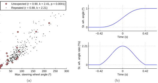
A few additional models were included. For the avoidance phase, an open-loop steering model was tested, in part because of its abovementioned prevalence in previous near-crash simulation, but further motivation was also found in the form of an observed correlation between maximum steering angle and maximum steering rate during avoidance; see Fig. 3.2a. This correlation, previously reported by Breuer [19], could be indicative of an open-loop,ballisticadjustment of steering wheel angle, where the final amplitude is determined before initiation (since adjustment speed predicts amplitude), with a duration that is independent of the amplitude (since the correlation is linear). Fig. 3.2b shows the specific steering adjustment profile adopted for the model in Paper V.
It had already been reported, in the author’s licentiate thesis [106], that the Salvucci & Gray model was capable of good fits of the observed stabilization steering. Further analysis indicated that this ability was mainly due to the model’s far point control, which had been shown, in the same thesis, to be equivalent to a type of yaw rate nulling
control: ˙δ=−Kψ˙, where ˙ψis the vehicle’s rate of yaw rotation. Therefore, such a model was tested directly.
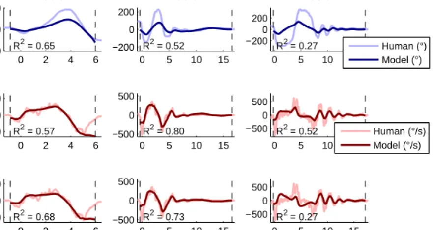
Interestingly, the very simplest models were found to work rather well, with the performance of the more advanced models to some extent being dependent on an ability to exhibit the behavior of the simpler models. Fig. 3.3 illustrates how the open loop avoidance model was, overall, the most successful at reproducing the avoidance steering behavior, despite its relatively small number of free parameters. The best-fitting version of the open loop model reached an averagecoefficient of determination R2, across
all drivers and recordings, of 0.75 (meaning that it explained, on average, 75 % of the variance in the data [43]). This version of the model relied on internal models of own and lead vehicle movements to determine the amplitude of steering. However, a simpler version, applying avoidance amplitudes as a linear scaling of lead vehicle looming on the driver’s retina, performed almost as well (averageR2= 0.71). The second best model
after the open loop model variants, the MacAdam model, was able to capture the observed pulse-like steering to some extent (averageR2= 0.49). However, for example the Salvucci
& Gray model, predicting ˙δrather thanδ, did not have this ability (averageR2= 0.20).
0 50 100 150 200 250 300 0 100 200 300 400 500 600 700
Max. steering wheel angle (º)
Max. steering wheel angle rate (º/s)
Unexpected (r = 0.90, k = 2.41, p < 0.0001) Repeated (r = 0.88, k = 2.21) (a) −0.42 0 0.42 0 1 Time (s) St. wh. angle (º) −0.42 0 0.42 0 2.21 St. wh. angle rate (º/s) Time (s) (b)
Figure 3.2: (a) A correlation observed in the ESC simulator study, between amplitude and rate of collision avoidance steering. (b) The steering of the tested open loop avoidance model, here shown with the duration that would, theoretically, yield the slope k of the repeated-scenario correlation in (a). For full details, see Paper V.
MacAdam Neff = 6 Average R2 = 0.49 −5 −4 −3 −2 −1 −100 0 100 R2 = 0.77 Example #2 Driver 3 (low exp)
ESC on −4 −2 0 −100 0 100 R2 = 0.52 Example #3 Driver 16 (high exp)
ESC off −4 −2 0 −100 0 100 R2 = 0.17 Exa