PERFORMANCE MEASUREMENT FOR HIGHWAY WINTER MAINTENANCE OPERATIONS
by
Lin Qiu and Wilfrid Nixon
Funded by the Iowa Highway Research Board Project TR 471
FINAL REPORT
IIHR Technical Report # 474 IIHR—Hydroscience & Engineering
College of Engineering The University of Iowa Iowa City, IA 52242
i TABLE OF CONTENTS
Chapter Page
1. INTRODUCTION ... 1
A. Motivation and Background ... 1
B. Challenges ... 2
C. Contributions... 4
2. LITERATURE REVIEW ... 5
A. Performance Measurement System: A Review of the Literature ... 6
B. Performance Measurement in Winter Maintenance Operations ... 6
C. Effect of Weather and Maintenance on Safety and Mobility ... 9
3. STORM SEVERITY INDEX ... 12
A. Storm Event Classification and Description ... 13
B. Development of a Multiple Regression Model that Produces the Storm Severity Index ... 16
C. Adjustment of Index by Expert Input ... 18
D. Result and Discussion ... 22
4. WEATHER AND TRAFFIC SAFETY ... 22
A. Method ... 23
B. Comparison Studies with Percent Change as the Standard Measure ... 29
C. Regression Studies Effect Size d and Percent Change as the Standard Measure ... 32
D. Results ... 33
E. Hierarchy Analysis Findings for Comparison Studies ... 36
F. Summary and Discussion ... 42
5. EFFECTS OF WEATHER AND MAINTENANCE ON ROAD SURFACE CONDITION ... 43
A. Method and Analysis ... 48
B. Results ... 48
C. Prediction Ability ... 63
6. EFFECTS OF WEATHER AND MAINTENANCE ON MOBILITY – STRUCTURAL EQUATION MODELING ... 65
A. Introduction ... 65
B. Method ... 67
C. Result and Analysis... 67
7. CRASH ANALYSIS DURING ADVERSE WEATHER ... 74
A. Introduction ... 74
B. Method ... 76
C. Results ... 76
ii
8. DEVELOPMENT OF A PERFORMANCE INDEX ... 89 9. SUMMARY AND CONCLUSIONS ... 92 REFERENCES ... 96 APPENDIX A: Methods used to determine the relationships between Road Surface
Condition, Weather, Traffic, and Maintenance Activities ...103 APPENDIX B: Methods used in Structural Equation Modeling ...109 APPENDIX C: Methods Used in Crash Modeling ...118
iii LIST OF FIGURES
Figure Page
3.1 Event classification ... 14
3.2 Modified Event Classification ... 15
3.3 Storm severity index distribution ... 18
3.4 Expert ranks for ten storm scenarios ... 20
4.1 Study outline ... 24
4.2 Effect of snow and rain on crash rate ... 35
4.3 Percent change in crash rate by decades ... 37
4.4 Effect of snow and rain on crash rate ... 38
4.5 The association between snow depth (1cm) with percent change of crash rate ... 41
5.1 CHAID diagram: first split by road surface temperature ... 52
5.1 Segmentation by OPERATION for the subgroup temperature 25°– 32°F ... 53
5.2 Segmentation by OPERATION and AADT category for the subgroup temperature 15°-25°F ... 54
5.3 Effect of Wind on RSC depends on levels of Wind and temperature ... 57
6.4 Weather and maintenance effects on mobility ... 66
6.2 Standardized solution of the structural model of effects of weather and maintenance on traffic mobility ... 68
6.3 Differential effects of storm events on speed by AADT, Road Class, Speed limit during different time of the day. ... 71
7.5 Weather and road surface conditions’ direct effects on safety ... 75
7.6 Weather and maintenance indirect effect through speed and volume ... 76
7.7 CHAID diagram of crash during normal driving conditions by AADT, ROAD CLASS, and speed limit. ... 81
7.8 Relationship between crash cross manner and surface condition ... 86
iv
LIST OF TABLES
Table Page
3.1 Modified scores for each storm Index factor ... 17
3.2 Storm scenarios description from the expert survey form ... 19
3.3 Average expert rank vs. storm index rank for ten storm scenarios ... 20
4.1 General information ... 27
4.2 Data information ... 28
4.3. Validity classification ... 28
4.4 Traffic volume reductionPvi due to different weather conditions ... 30
4.5 Crash rate change compare to non-adverse weather conditions ... 34
4.6 Percent change of crash rate (fatal, injury and PDO) by decades ... 36
4.7 Percent change of injury rate by decades for rain ... 36
4.8 Percent crash and injury rate change for snow and rain by country ... 38
4.9 Effect size d for each study ... 40
4.10 Meta-analysis by effect size d ... 40
4.11 Meta analysis by percent change in crash rates ... 41
5.1 Summary of Measures ... 49
5.2 Risk Estimate of the Classification Tree ... 55
5.3 Effect of weather ... 57
5.4 Effect of maintenance at three operations stages ... 61
5.5 Effect of traffic volume ... 63
5.6 Prediction results of maintenance actions based on the MLR model ... 64
6.1 Estimated coefficients for subgroups ... 72
7-1 Preliminary MCA results ... 77
7.2 Probability of injury and PDO involvement during adverse weather conditions ... 79
7.3 Road attributes of selected highways ... 80
7.4 Probability of Injuries and PDOs during normal driving conditions ... 82
8.3 Speed targets for different operational stages by road class, speed limit, ADT and time of the day ... 90
8.2 Base Speed Reduction (mph) for Road Priorities ... 91
1
1. INTRODUCTION
A. Motivation and Background
Although winter highway maintenance has improved significantly over time (for instance, between 1995 to 2001, there was a 26% decline in crashes during sleet and snow weather conditions (Goodwin, 2003)), road users still experience delays and crashes due to unsatisfactory road conditions that result from poor winter weather. In 2001, approximately 1000 people were killed and 95,000 people were injured in crashes on snowy and slushy pavement (FHWA, 2002). Annually there are 500 million hours of delays in major US highways due to adverse weather conditions (NOAA, 2002). While maintenance operations aim to provide road users with a safe highway that has limited delays, to achieve this condition maintenance agencies spend 2.3 billion dollars annually on Winter Highway Maintenance (FHWA, 2002). Given this high expenditure, an important goal for a winter maintenance agency is to find the optimal usage of limited resources. One way to reach this goal is to develop a performance measurement system. Such a system is typically composed of a series of quantitative measures that evaluate how well maintenance activities have been performed to meet a variety of road users’ expectations (Adams, 2003). By comparing the real-time performance outcome data with the pre-specified targets, performance measurement can inform winter maintenance agencies how well an operation has been conducted to improve mobility and safety. The feedback from the performance measures will help an agency to improve their maintenance actions over time.
The generally identified goals in the management of transportation systems are safety, mobility, effectiveness, environmental concern, and user-satisfaction. The two major goals of winter highway maintenance are safety and mobility. The commonly used outcome measures for mobility and safety are traffic speed and traffic flow rate and accident rate. However, in winter maintenance, it is more typical to measure either outputs (evaluate the result of maintenance activities, such as, cycle time, lane-miles
2
maintained) or different outcome measures (e.g. road surface condition observations or pavement friction). Output measures are often relatively simply to collect, but they are not directly tied to maintenance goals and objectives and cannot be easily communicated to road users. Likewise, the outcomes currently used are not necessarily easy to collect, nor are they easily translatable into a publicly accepted form of outcome measure.
Based on the current literature search, it is clear that though there is a reasonable amount of performance measurement studies conducted in the winter maintenance area, few of them are comprehensive enough to evaluate winter maintenance outcomes (how safe and mobile traffic was able to get to its destination), while at the same time taking weather condition(the severity of individual storms), the specifications of road system being treated(Interstate or Primary, different AADT levels), various traffic specifications (urban vs. rural, day vs. night, traffic vs. non-peak, etc.) and the maintenance effort (frequency of plowing actions, quantity of chemicals, and other operational input) together into consideration.
To establish a performance measurement system for operational use, the proposed performance measurement system needs to take those factors above into consideration. Among the above factors, weather conditions, specifications of road system characteristics and traffic specifications (Peak-hour or not, Day time or not) are used in this study as normalizing factors or classification variables to ensure an appropriate comparison across different storm events and maintenance routes. Maintenance input measures the cost to agencies in fighting a storm, which is a major concern and easy to quantify, but not a dominant factor. Measures of winter maintenance outcomes is the most important factor, and can also be understood as the value-added benefit to road users by improved traveling conditions.
B. Challenges
There are two particular challenges when trying to develop a performance measurement system. First of all, maintenance efforts and outcomes are largely dependent on the variability of individual storms. Therefore to make the maintenance effectiveness comparable across different storms, the individual storm severity must be quantified. However, until this study, there were no examples of storm severity indices
3
that measured severity on a storm by storm basis. Such weather indices measured behavior over a total winter season.
Second, the complexity of relationships involved in the performance of the winter maintenance operations means that they are not only dependent on the maintenance input or effort, but they are also sensitive to all the other conditions, including weather severity variables, road classifications, and various traffic specifications. Thus, different targets need to be developed to accommodate these differences. The appropriate targets can only be set based on a sound understanding of these relationships. Even though there are some studies that examine the effect of weather on mobility and safety, the research findings on the effect of weather on safety are quite conflicting. Also, there is an absence of studies that examine the effects of maintenance actions (Andrey, 2003), and no studies model how the effects of maintenance and weather changes with the various conditions mentioned above.
On the basis of these needs and challenges, this project constructs a performance measurement framework for the winter maintenance operational system. Operational goals have been established. Measures that evaluate the maintenance outcomes, as well as those sets of measurement variables upon which the winter highway maintenance outcomes depend have been identified and included in the performance measurement framework.
Chapter 2 reviews the existing literature in the field, including general guidelines for performance measurement, and current performance measurement in winter highway maintenance practice. The review also identifies deficiencies in current practice. Further, literature on the effects of weather and maintenance operations and their complex interactions on safety and mobility have been reviewed.
Chapter 3 develops a storm severity index used to quantify the severity of individual storms. Multiple regression is used to built the model and the model was validated by expert feedback.
Chapter 4 generalizes the current conflicting results of studies that have examined weather effects on safety. A hierarchical meta-analysis is applied. Effect size and proportional change in crash rates were used to standardize findings.
4
Chapter 5 investigates the effects of weather factors and maintenance actions on road surface conditions, and tests the possible interactions between these two sets of variables. CHAID (Chi-squared Interaction Detection) was applied in this step to identify the significant factors and interactions. MLR (Multinomial Logistic Regression) was used further to validate the result produced from CHAID, and quantify the effects.
Chapter 6 explores the direct and indirect casual effects of weather and maintenance actions on mobility and safety. Also the important interactions between light, and road classifications were tested and included in the models. Structural Equation Modeling (SEM) was used in this chapter to estimate the direct and indirect effects.
Chapter 7 presents the final performance measurement model, and shows typical results that would be obtained from the model. The results are evaluated by comparison with field data. This comparison shows that the performance model that has been developed is an effective measurement tool and can also be used for the planning use.
Chapter 8 presents conclusions of the project, together with recommendations for further work.
C. Contributions
This proposed measurement system can be used to enable winter maintenance agencies to evaluate how well operations have been conducted to meet road users’ needs as specified in maintenance goals (as used for the post-event evaluation) by comparing the maintenance outcomes with the specified standards. Combining the modeling results, this work can enable the decision maker to determine the optimum decision through balancing the trade-offs between maintenance input and road user benefit in terms of traveling comfort and safety.
The constructed prediction model in chapter 5 can be used to predict the road surface condition for a specified weather event given the traffic volume and maintenance procedures. The structural equation modeling results have established the effects of maintenance actions, weather conditions, and road surface conditions on traveling speed and volume and crash rates. Thus for a specified weather event, a given time of the day, and a given road class and AADT, the model can estimate the traveling speed and traffic volume, as well as crash rates with different maintenance operation input. Thus, this
5
model is a predictive tool for maintenance managers, and as such allows them to conduct “what if” experiments that will lead to optimization of maintenance practice over time.
Clearly, observations of the road surface condition will continue to be effective measures of maintenance outcomes in the near future. Thus road surface condition prediction based upon maintenance and weather conditions can be used by the maintenance agency to do pre-event evaluations, and to evaluate and facilitate the selection of the best strategies for a variety of scenarios. This established relationship between road surface condition and the speed and volume could be used as the rationale to establish a Mobility index (such as that used in MDSS, Mahoney, 2005). Further, the relative magnitudes of the effects of different maintenance methods on mobility and safety that is predicted by the models will enable agencies to assign priorities, and to compare maintenance outcomes based on the input resource.
Moreover, the study results can also be used to go from asking how maintenance affects mobility and safety to understanding how to maximize limited resources so as to improve maintenance effectiveness. For instance, by studying the relationship between performance outcomes and weather severity, road scope, and all the other variables, this study found some areas for potential improvement in current winter maintenance practice. On this basis, a series of recommendations for possible change in operational methods are presented herein.
2. LITERITURE REVIEW
This chapter covers the review of methods and guidelines for establishing an applicable performance measurement system. Studies of the current performance measurement practice in the winter maintenance field have been summarized and deficiencies have been identified. All the major components of performance measurement systems and how they and their interactions affect maintenance outcomes have been reviewed. Additionally, studies on the weather and maintenance related impact on road mobility and safety have been reviewed.
Information on the framework construction of performance measurement systems helps to identify the necessary components of such systems. The literature review on
6
winter maintenance operations identified that the most widely used performance measures used in these operations are various measures of road surface condition. While such measures have the advantage of being relatively easy to collect and thus easy to use operationally it should be noted that such measures are not directly related to safety and mobility goals.
A. Performance Measurement System: A Review of the Literature
Performance measurement is a well-established concept in the transportation arena. The Federal Highway Administration (FHWA) has already conducted many studies on performance measurement. According to the FHWA definition (FHWA, 2004): “Performance measurement is a process of assessing progress toward achieving predetermined goals.” Generally the following broad categories would be useful to identify goals for performance measures: Safety, Accessibility, Mobility, Environmental and resource conservation, and Operational efficiency (NCHRP, 2000).
Well-designed performance measures should be linked to objectives and goals (Neely, 1997). For instance, the likely performance measure to meet the goal of safety are rate of highway-related fatalities/ injuries (number of accidents per 100 million vehicle miles traveled) (FHWA, 2003). The likely performance measures for the goal of mobility are travel speed, delay, and quantity of travel (Vehicle miles traveled-VMT), and Average Annual Daily Traffic (AADT), together with both variability and reliability indexes (NCHRP, 2003). The likely measures for productivity and environmental conservation are monetary values for the maintenance agencies and society.
Principles in guiding performance measures selection have been discussed in a number of studies (Meyer 1995, TRB 2001, and Neely 1997): Performance measures should be customer-oriented and outcome-based (TRB, 2001). In addition to the traditional use of output-based performance measures that measure the product or service of the activity, outcome measures that measure progress toward achievement of the purpose should be combined with output measures (Cambridge, 2001). Generally, performance measures are classified in the following categories:
7
• Input measures, indicating the amount of resource used (such as types and quantity of material, frequency and types of mechanical removal, labor, equipment, etc.);
• Uncontrollable factors, indicating those factors that organizations can’t change but contribute to the decreases of performance. ( such as natural hazard and emergency, etc);
• Output measures, indicating effectiveness of resources transformed to service. ( such as road surface condition, maintenance cycle time)
• Outcome measures, directly reflecting operation impact on goals (such as improved mobility and safety, or lower travel costs to customers).
To develop a comprehensive performance system, the above factors must be taken into account. The input measures are directly associated with agency spending, and the outcome measures clearly reflect how well operations meet the organization goals and customer expectations. Moreover, to make the selected performance measures applicable in operations, data availability, sample size, and frequency of measurement are all major considerations.
B. Performance Measurement in Winter Maintenance Operations
Maintenance operations are typically performed to minimize the adverse weather effects on traffic in terms of traveling speed, and volume, and to minimize the adverse weather effects on safety in terms of crashes. Effective performance measures have significant importance to any agencies involved in winter maintenance. Through measuring performance, a maintenance agency will be able to make more informed decisions, and to track the process over time toward a goal or objective (TRB, 2001). A variety of performance measures have been developed for different purposes in the winter maintenance area. For instance, Adams et al. (Adams, 2003) explored the business uses of data gathered by a new winter maintenance vehicle equipped with AVL (automated vehicle location) system, GPS (global positioning system) receivers, and material sensors and provided systematic performance measures for budgeting and monitoring use. To best meet the customer expectation, Caltrans (California Department of Transportation) collected data from a public satisfaction survey, and used a custom rating scale to
8
evaluate operational effectiveness (Kuhl, 2000). Taking public perception into decision making can be good. However, public opinions may depend on personal preference and it is hard to evaluate each storm by survey.
This study is focused on evaluating the effectiveness of winter highway maintenance operations and as a result to facilitate decision making. The primary goal for winter highway maintenance operations is to reduce undesirable road surface conditions. By doing so, an agency can reduce accidents and minimize delays and changes in travel times compared to normal weather conditions. As the public survey results indicated, the goal of safety and mobility are also the road user’s primary concerns (Alfelor, 1999). Perhaps the most relevant study is by Blackburn. For the purpose of evaluating the effectiveness of maintenance strategies and tactics, Blackburn established a Pavement Ice Condition Index (PSIC) by visual characterization of roadway surfaces descriptions (amount of ice/snow/slush on the road surface and condition of the interface: bonded or un-bonded). PSIC can be used to evaluate the during-storm performance, and the time needed to achieve a certain PSIC can be used to evaluate after-storm performance (Blackburn, 2004). This kind of road surface description is a typical measure to evaluate operation effectiveness around the world because of its ease of understanding and comparatively low cost to obtain, and also because it is associated with the maintenance end-goal of mobility and safety to some extent. However, there are two deficiencies associated with this measure. First, the measure, based on crew observation, is subjective. Second, the road surface description is not direct enough to indicate the safety and mobility effects to road users (speed, accident rate, traffic volume).
As proposed by Nixon, friction is another promising indicator of road condition (Nixon, 1998). The measure of the friction ranges between 0 and 1, with 0 indicating most slippery icy surface, and 1 indicating normally dry surface condition. Friction is normally measured by a locked-wheel skid-resistance device attached to the maintenance truck or patrol vehicles (Hagiwara, 1990). Finland has established Winter Maintenance Level-of-Service based on the friction value (Leppannen, 2001). Japan has constructed a traffic accident reconstruction model, and it is noted that improving friction value of the pavement could greatly influence the safety especially when the friction value is around 0.2 (Hosseinlou, 2000). However, the correlation between friction levels and traffic
9
speed/volume is still less than clear, and a reliable friction measurement device is still in the development stage for heavily traveled highways (Al-Qadi, 2002).
C. Effect of Weather and Maintenance on Safety and Mobility
Generally the number of crashes during a certain time unit is related to many factors, such as driver behavior, geometric characteristics, e.g. grade and curve radius, weather related variables, interactions between geometrics and weather, etc. (Shankar V, 1995). Other important interactions have been identified in the literatures including interactions between weather and traffic volume, holidays and weekly patterning of social activities e.g. weekday travel patterns (Levine et al., 1995).
Sometimes researchers use crash rate, which is the ratio of crash counts and traffic exposure (flow rate, namely traffic volume per lane) as the measure of crashes (Amoros, 2002). Mean speed and variation in speed are found to be positively related to crash rates (e.g. see Garber and Gadiraju, 1990; Garber and Ehrhart, 2000; Dickerson et al., 2000). Also the effects of speed and traffic flow rate on crash rates depend on the type of highway (Garber and Ehrhart, 2000). In terms of crash severity, Golob and Recker (2003) found that more adverse conditions were associated with the lowest traffic volumes and high variations in traffic flow. Other studies that have modeled the relationship between road accidents and traffic flows are Dickerson et al. (2000) and Martin (2002).
Effect of Weather on Crash Rates
Research on crashes during adverse weather conditions suggests that adverse weather is associated with an increase in the number of less severe crashes, such as minor injury and property damage only crashes (Andrey, 2003). However, adverse weather has only a minor influence on severe crashes, severe injury or fatal crashes. For instance, Evans (1991) stated that “the effect of inclement weather [snow fall] is more to reduce mobility by deterring travel or reducing speeds than to change safety [fatality].”
Snow event type and poor visibility were found to be associated with both reductions in speed and increase of variation in speed (Idaho 2000, Liang 1998) ). Moreover, the effect of rain depends on the time of the day. Keay (2005) found a 5.2% increase in crash rates at night compared to a 1.9% increase during the day. The effect
10
also depends on the characteristics of the weather event (Andrey, 2003), and geometric and ambient temperature-related variation (Shankar V, 1995) and specific site or city characteristics. Eisenberg (2005) and Suggett (2002) both found that the risk of fatalities is significantly higher on the first snowy day of the season compared to subsequent snowy days during the same season.
In terms of crash characteristics, (Andrey, 2003) “Snow events are associated with disproportionately more single vehicle crashes; more collisions at locations without traffic control and on roads with speed limits of 60 kph or higher; and they are less likely to involve a turning maneuver than ‘normal’ driving.” These findings have been confirmed by other studies (Mercer, 1986; Andrey, 1989). Lane (1995) found “passing and lane changing were especially hazardous in winter driving conditions and the risk was increased by the tendency of slush and snow to build up between the right and left lanes and on the shoulders. Excessive vehicle speed for inclement roadway conditions was a factor in most of these crashes”.
In terms of precipitation type, Suggett (2002) has found crash risk is particularly high for freezing rain or sleet events, and low for drizzle or dry snow. In addition it has been demonstrated that even after precipitation ends, crash risks stay elevated. One possible reason is the accumulated precipitation may lead to slippery road surface conditions, a conjecture that this dissertation research examines further. The studies exploring the interactions of weather with other factors on crash rates suggest that the effect of weather type (rain/ no rain) depends on the rural or urban settings. Bertness (1980) found over 100% more vehicle accidents under rain compared to non-precipitation, particularly in urban areas, but the accident severity associated with rain was greater in rural areas.
Effect of Weather on Traffic Volume
Travelers can and do defer their trips during adverse weather. During rain fall, traffic volume on the highway decreases 1.35 to 2% depending on the precipitation rate. It also changes considerably with time of the day (Keay, 2005; Doherty et al. 1998, Colding, 1974). During snow fall, traffic volume decreases substantially from 7% to 56% (Hanbali, 1994) and 10% to 50% (Knapp, 2001).
11
In terms of the distribution of the traffic volume, it is likely to observe more frequent very low traffic volume, less frequent very high traffic volume during snow than non-precipitation or rain (EIDessouki, 2004).
Effect of Weather on Traveling Speed
There have been several studies that examined the relationship between weather and speed. Snow events and poor visibility were found to be associated with both reductions in speed and increase of variation in speed. For instance, the 2001 Traffic Flow Theory and Highway Capacity manual provide models that predict the average off-peak winter weather vehicle speed reduction is 3.9 mph for low visibility (visibility below 0.4 km/0.25 mi) and 7.3 mph for snow cover on road ways. Brown and Baass (1997) found a 10% to 30% reduction in free flow speed. Liang (1998) found a three times larger variation in speed during a snow event.
Moreover, these studies suggest that the decrease in speed and increase in speed variation during snow storms are influenced by road classification and vehicle type (passenger car or pick up trucks) (Padget 2001, Liang 1998). For instance, Hanbali and McBride (1994) found snowy/icy conditions are associated with an average 18% to 42% speed reduction on two-lane highways and 13% to 22% reduction on freeways (More reduction on lower level of road).
In a summary, previous literatures demonstrate clearly that speed and volume and various variations of the indexes (reliability index, miserable index, etc.) are critical measures of mobility. Crash rates (fatality rate, injury rate, property-damage-only rates) and levels of severity are critical measures of safety. However, to incorporate these measures into the performance measurement process of winter highway maintenance operations requires filling two main gaps.
First, Road Surface Conditions (RSC) as the traditional measure of maintenance outcome will continue be used as the primary performance measure in winter highway maintenance operations due to its low cost to obtain, and ease of use in making maintenance operation decisions. However, to date, there are not enough sound studies that link different types of RSC with direct measure of mobility and safety (speed, volume and crash rate). Lack of the studies in these areas make the evaluation of
12
maintenance outcome obscure to road users and maintenance agencies, and makes the process of meeting the goals of mobility and safety more difficult.
Second, even when hourly measurement of speed and volume are possible to obtain, and maintenance agencies are willing to use speed and volume as their primary measure of the operational effectiveness, no study to date has accommodated appropriate targets with which real time performance measurement can be compared. Setting up the appropriate targets against which performance can be compared can be a daunting task, because it must be based on a thorough understanding of the system. However, there are no studies that quantify the influence of types and levels of maintenance methods on speed, volume and crash rates. Even though many studies examined the effects of adverse weather conditions, few of them include winter maintenance in to considerations. However, maintenance operations and weather conditions together influence the road surface conditions, and through changing road surface conditions, maintenance and weather have influence speed and volume and crash rates. Studies on effects of weather suggest that wind speed, precipitation, surface temperature, and visibility are all associated with different levels of reduction in speed and volume. Also interactions effects with light, Urban/Rural, Road Class etc. need to be taken in to consideration as well.
3. STORM SEVERITY INDEX
As discussed in the earlier chapters, in order to determine the performance of an agency in dealing with a particular winter storm it is critical that the severity of the storm be quantified in some way, so that the performance can be normalized with respect to the severity of the weather. In this chapter, the process of developing such an index is described, and the storm severity index is presented. The storm severity index quantifies to what extent an individual storm poses difficulty to maintenance activities.
No study to date has evaluated the severity of individual storms as opposed to the severity of the whole winter season. Decker, 1998 developed a weather index, which incorporates daily new snow fall into consideration; but this is still a winter season based index. The only relevant studies are those that describe individual storms by
13
meteorological factors. One such is the storm description matrix developed in the FHWA Manual on Anti-Icing Practice (1996). Nixon and Stowe (2004) improved and extended the storm description matrix by incorporating pre and post storm behavior in the matrix.
The development of the storm severity index was conducted in three steps. First the appropriate storm event classification and descriptions were developed. Second, based on the storm description, a multiple regression model was built to produce a storm severity index between 0 and 1. Third, representative storms were ranked in severity by winter maintenance supervisors and the model was modified to reflect this ranking. The storm severity index thus produced can be used as an objective measure of the challenge that an individual storm poses to a maintenance agency.
A. Storm Event Classification and Description
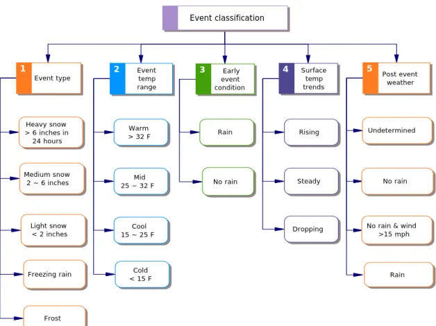
The matrix of possible storms developed by Nixon and Stowe (2004) can be represented schematically as shown in Figure 3.1. This is based upon the storm matrix in the FHWA manual on anti-icing practice (1996), but extends it especially in how it considers pre- and post-storm behavior. By combining one from each of the five categories or factors, a large number of potential storms can be described. Nixon and Stowe (2004) discarded some unlikely storm scenarios and considered a total of 312 storm scenarios (96 for each of the snow events, and 12 each for the frost and freezing rain events).
14 Event classification 1 Event type Heavy snow > 6 inches in 24 hours Medium snow 2 ~ 6 inches Light snow < 2 inches 2 Event temp range Warm > 32 F Mid 25 ~ 32 F Cool 15 ~ 25 F 3 Early event condition Rain No rain 4 Surface temp trends Rising Steady Dropping 5 Post event weather Undetermined No rain
No rain & wind >15 mph
Freezing rain
Frost
Cold
< 15 F Rain
Figure 3.1. Event classification
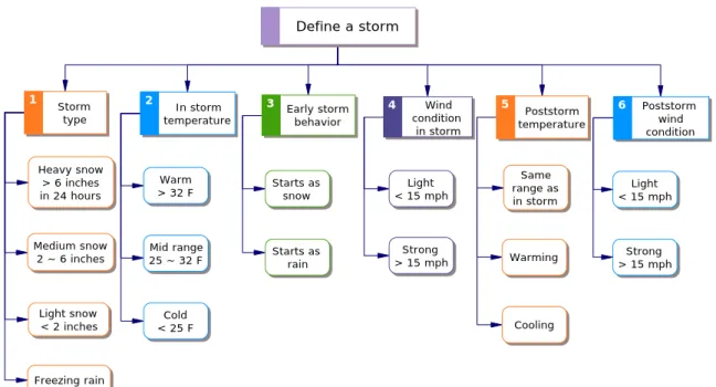
For the purposes of generating the storm severity index, these storm scenarios were adapted as discussed below.
1. Because the focus of this effort was on storm events, it was decided to remove frost as a possible event type. Thus only four possible storm event types were considered: heavy snow, medium snow, light snow, and freezing rain.
2. Because the levels of wind during a storm can have a significant impact on the challenges faced while maintaining roads during the storm it was decided to incorporate the in-storm wind condition as another factor. Wind condition during a winter storm is an important factor to be taken into account, because wind speeds in excess of about 12 to 15 miles per hour may cause drifting snow problem and when the pavement is wet, cause retention of snow (e.g. see Illinois DOT, 1998).
15
3. It was decided to simplify the options for temperature ranges from four ranges (warm, mid, cool and cold) to three ranges by combining the cool range (15°F ~ 25°F) and the cold range ( < 15°F ) into one single range (< 25F ) in this classification. Thus the storm severity index has only three temperature ranges – warm, mid, and cool.
4. The post-storm conditions seemed overly complex for the purposes of the storm index, and accordingly these were simplified into two categories rather than four. Thus the four conditions from Nixon and Stowe (2004) of “Undetermined”, “No rain”, “No rain with wind above 15 mph”, and “Rain”, are simplified to “Light wind” and “Strong wind” instead, because the impact of post-storm winds was considered to be much more important than the impact of post-storm rains. After these modifications, the event classification used in this study is as shown in Figure 3. 2.
Define a storm 1 Storm type Heavy snow > 6 inches in 24 hours Medium snow 2 ~ 6 inches Light snow < 2 inches 2 In storm temperature Warm > 32 F Mid range 25 ~ 32 F Cold < 25 F 3 Early storm behavior Starts as snow Starts as rain 4 Wind condition in storm Light < 15 mph Strong > 15 mph 5 Poststorm temperature Same range as in storm Warming Cooling 6 Poststorm wind condition Light < 15 mph Strong > 15 mph Freezing rain
16
B. Development of a Multiple Regression Model that Produces the Storm Severity Index
Using the above modifications, any given storm can now be described in terms of six variables: ST (Storm type); Ti (In storm road surface temperature); Wi (In storm wind condition); Bi (Early storm behavior); Tp (Post storm temperature); and Wp (Post storm wind condition). In order to develop a storm severity index between 0 and 1, each condition for the six variables must be assigned a score, and these scores must then be combined in some manner to create a composite score. This composite score can then be normalized so as to create the storm severity index.
The format of the storm severity index was based upon that used by SHRP-H-350 (Boselly, et al. 1993) for the development of a winter severity index. Thus the general form of the index equation is given as:
5 . 0 ] ) * * [( * 1 ⎥⎦ ⎤ ⎢⎣ ⎡ − + + + = ST Ti Wi Bi Tp Wp a b SSI Eq. 3.1
Where SSI is the storm severity index and a, b are parameters to normalize the storm severity index from 0 to 1.
The storm type is clearly modified by the road surface temperature and the in-storm wind condition, thus these three terms are multiplicative. The various pre- and post-storm behaviors are considered, in contrast, to be additive to the main storm and are expressed as such in equation 1. The two constants “a” and “b” are used to normalize the storm severity index between 0 and 1.
Once the form of the equation is established, the relative scores between the values of the factors must be estimated. This involves attempting to assess how much worse a cold storm (with road surface temperatures below 25º F) is to handle than a warm storm (with surface temperatures above 32º F). A first approximation of these values can be obtained by studying the FHWA Manual of Practice recommended treatments (1999) and comparing how (for example) road temperature impacts treatment amounts and frequency, but this provides only an initial estimate. These initial estimates are listed in Table 3.1 (see below).
17
Table 3.1. Modified scores for each storm index factor
Storm Type Freezing rain Light Snow Medium Snow Heavy Snow
0.4 (0.72) 0.35 0.65 (0.52) 1
Storm Temperature
Warm Mid Range Cold
0.25 0.6 (0.4) 1 Wind Conditions in Storm Light Strong 1 1.2 Early Storm Behavior
Starts as Snow Starts as Rain
0 0.1
Post Storm Temperature
Same Warming Cooling
0 -0.087 0.15 Post Storm Wind Conditions Light Strong 0 0.15 (0.25)
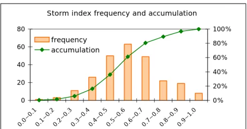
*Values inside parentheses indicate values modified after the Supervisors’ evaluations. After these initial values had been applied, the model was adjusted to get an approximately normal distribution. Using the estimates for the six factors listed in Table 3.1., the storm severity index was calculated for 252 different storms based on the initial algorithm and scores. Then the initial scores were modified (using the “a” and “b” constants) so that the computed storm severity index values have an approximately normal distribution (as shown in Figure 3.3.) The scores used for the six factors are shown in Table 3.1.
18
Storm index frequency and accumulation
0 20 40 60 80 0.0~0 .1 0.1~0. 2 0.2~ 0.3 0.3~ 0.4 0.4~ 0.5 0.5~ 0.6 0.6~ 0.7 0.7~0 .8 0.8~0. 9 0.9~ 1.0 0% 20% 40% 60% 80% 100% frequency accumulation
Figure 3.3. Storm severity index distribution C. Adjustment of Index by Expert Input
To test and improve the accuracy and reliability of model, in the final step, ten storms were selected and were ranked in severity by winter maintenance garage
supervisors. The ranks produced by the index were compared with the expert ranks provided by the supervisors. The major differences were discussed and the model was adjusted to ensure storm index ranks agree with the expert ranks.
Selected ten storms ranked in severity by Winter Maintenance Supervisors
Ten representative storm scenarios were selected out of 252 possible storm events and described in a survey form (Table 3.2). The storms were labeled A through J and their order on the survey form was randomized so as to minimize bias. Maintenance supervisors in Iowa ranked these ten scenarios according to the level of difficulty that these events would pose to them in their maintenance activities. The hardest was ranked as 10, and the easiest as 1. The storms were ranked by 38 supervisors around the State of Iowa.
19
Table 3.2. Storm scenarios description from the expert survey form Storm
scenarios Description: A
A storm with freezing rain and temperatures in the warm-range (above 33 Fo) that starts as rain. Winds in the storm are strong (over15mph). After the storm, winds become light and temperatures warm up.
B
A storm with heavy snow (above 6 inches) and temperatures in the midrange (25Fo to 32Fo) that starts as snow. Winds in the storm are strong (over 15 mph). After the storm, winds become light and temperatures cool down.
C
A storm with heavy snow (above 6 inches) and temperatures in the warm-range (above 33Fo) that starts as rain. Winds in the storm are light (less than 15 mph). After the storm, winds become strong and temperatures cool down.
D
A storm with heavy snow (above 6 inches) and temperatures in the warm-range (above 33Fo) that starts as snow. Winds in the storm are light (less than 15 mph). After the storm, winds become strong and temperatures cool down.
E
A A storm with light snow (up to 2 inches) and temperatures in the warm-range (above 33Fo) that starts as snow. Winds in the storm are light (less than 15 mph). After the storm, winds remain light and temperatures warm up.
F
A storm with freezing rain and temperatures in the cold-range (15Fo to 25Fo) that starts as rain. Winds in the storm are light (less than 15 mph). After the storm, winds remain light and temperatures remain cold.
G
A storm with medium snow (2 inches to 6 inches) and temperatures in the midrange (25Fo to 32Fo) that starts as snow. Winds in the storm are light (less than 15 mph). After the storm, winds become strong and temperatures warm up. H
A storm with medium snow (2 inches to 6 inches) and temperatures in the midrange (25Fo to 32 Fo) that starts as snow. Winds in the storm are light (less than 15 mph). After the storm, winds remain light and temperatures remain in the midrange.
I
A storm with light snow (up to 2 inches) and temperatures in the midrange (25Fo to 32 Fo) that starts as rain. Winds in the storm are light (less than 15 mph). After the storm, winds remain light and temperatures warm up.
J
A storm with heavy snow (above 6 inches) and temperatures in the cold-range (15Fo to 25Fo) that starts as rain. Winds in the storm are strong (over 15 mph). After the storm, winds remain strong and temperatures remain cold.
Storm index ranks in comparison with expert ranks
The rankings of the ten storms were then compared with the initial storm severity index produced by the model. Table 3.3. shows the average rank that the 38 supervisors assigned to the ten storms, together with the rankings developed from the initial form of the storm severity index. It is clear that while there is general agreement between the
20
supervisors and the initial index, there are also areas of significant disagreement, as discussed further below.
Table 3.3. Average expert rank vs. storm index rank for ten storm scenarios
A more complete (and also more complex) representation of the responses obtained from the supervisors is given in Figure 3.4.
Figure 3.4. Expert ranks for ten storm scenarios
The ten storms are listed on the x-axis in Figure 3.4., and for each storm the solid black line is the mean response. The box represents the upper and lower quartiles, and the
Storm scenario E A I H G F D C B J
Storm Index rank 1 2 3 4 5 6 7 8 9 10
21
bars represent the high and low data values. The other symbols represent statistical outliers that were discarded from the final analysis.
Model adjustment to ensure storm index ranks agree with the expert ranks
As indicated in the above section, there was less than perfect agreement between the initial storm severity index and the supervisor rankings. Three major areas of difference are considered below. On the basis of this comparison, the numerical values for certain of the factors were adjusted so that the storm severity index scores for these ten storms are now in agreement with the rankings given by the garage supervisors.
1. Scenarios A, I, and H: Storm Scenario A (freezing rain) was ranked as more severe than storms H (medium snow) and I (light snow) by the supervisors, which contrasted markedly with the initial severity index. This indicated that the score assigned to freezing rain was relatively low and the score for medium snow was relatively high. The scores were adjusted accordingly (see the values in parentheses in Table 3.1).
2. Scenarios D and B: There was a significant degree of disagreement between the supervisors with regard to storms B and D. 63% of the supervisors ranked Storm scenario B as less severe than storm scenario D while 27% of the supervisors took the opposite view. It appears that the majority of supervisors think that post-storm winds are worse operationally than in-storm winds. On the basis of this, the score for post-storm winds was increased (see the values in parentheses in Table 3.1).
3. Scenario F, D, and B: Storm scenario F was ranked as more severe than storms D and B by the supervisors, again in contrast to the initial storm severity index. It appears that the lower temperature and the freezing rain condition (the latter as noted above) are considered to be operationally more severe conditions than a heavy snow storm. Thus the score for mid-range storm temperatures was also adjusted.
As indicated in the above analysis, the discordant scores have been adjusted according to the supervisor rankings. The adjusted scores are the scores inside the parentheses, shown in Table 3.1. While the index now matches the evaluations of winter maintenance supervisors in Iowa, it is not clear how well it would match with evaluations of similar supervisors in other Mid-western States (who would experience similar
22
weather but may have differing operational responses) nor how it would compare with evaluations from supervisors from other climatic regions (e.g. Mountain States). While such comparisons are clearly of interest, they lie beyond the scope of the current study.
D. Result and Discussion
This chapter presents a model that takes the weather factors as the input and produces a storm severity index from 0 to 1, with 0 indicating very mild storm and 1 indicating very severe storm. The initial regression model was given as Eq. 3.1 and the assigned values are given in Table 3.1.
Using this model, the storm severity index for 252 different storm events can be provided. The index was compared with rankings provided by winter maintenance supervisors from the Iowa Department of Transportation, and was adjusted to agree with those rankings.
Development of the storm severity index is the first step in measuring the performance of winter maintenance operations. The index measures the level of difficulty that each individual storm events would pose to a maintenance agency in their maintenance activities. Thus it can be viewed as a normalizing factor that provides a basis for the fair comparison of the performance of maintenance operations under differing weather conditions.
4. WEATHER AND TRAFFIC SAFETY
Adverse weather conditions are known to be a major factor impacting traffic safety and mobility. A number of studies have attempted to quantify this impact, although the results of these studies are not consistent. The increased crash rate ranges from less than 100% to over 1000% during snowfall. There is also a debate on whether injury rate decreases during snowfall. Andrey (2002) noted that injury rate increased over 20% in Ottawa, Canada. Brown and Baass (1998) found fewer crashes involving injuries during winter in Quebec, Canada. The impact of severe weather on fatal crashes is even harder to quantify, because of the lower number of events involved and other confounding factors. Eisenberg and Warner (2005) estimated the effects of snowfall on US traffic
23
crash rates between 1975 and 2000, and concluded that fatal crash rate decreased during snow days compared to dry days, but nonfatal-injury crash rate and property-damage-only crash rate increased, which seems to be in agreement with Knapp et al’s (2000) study in the state of Iowa.
To present a clear idea of how weather impacts traffic safety, the method of meta-analysis has been applied to examine the impact of adverse weather on crash rates. The basic idea of meta-analysis is to identify relevant studies by a systematic search and then use effect size standardizing on each study result. In addition, this approach corrects sampling error and other artifacts and can present an estimate of the total effect with minimized subjectivity (Hunter et al., 2004). Further, since different studies might be influenced by methodologies, time span and regions, hierarchy meta-analysis has been applied using these factors as grouping variables. Separate analyses are conducted for each group.
A. Method
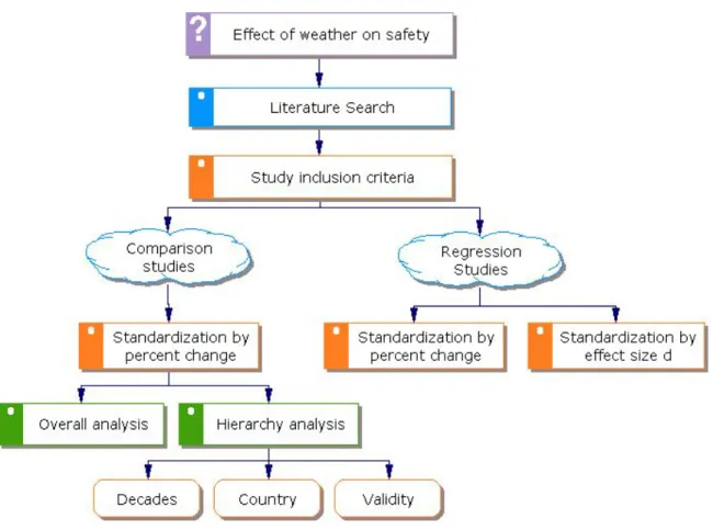
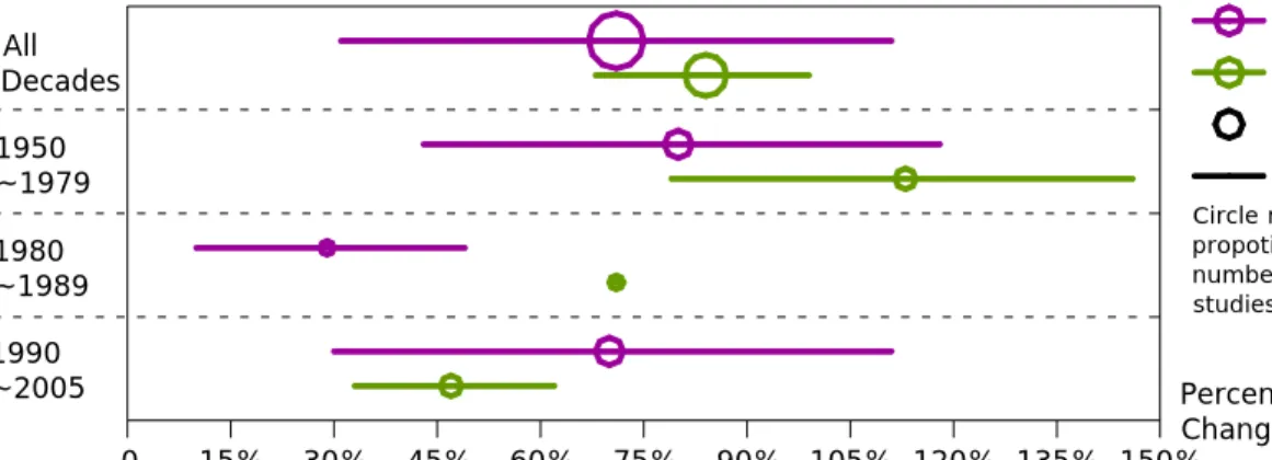
The process used in the meta-analysis is outlined in Figure 4.1. After careful review of the included articles, two meta-analyses were conducted separately for comparison studies and regression studies. The first step was to conduct a comprehensive literature search. An inclusion criterion filter was then applied to the found literature. After careful review of the included articles, two separate meta-analyses were conducted for “comparison studies” and “regression studies”. Here, the “comparison studies” indicates those studies using binary weather indicators, for instance, comparing daily crash rates during snow and those during a non-snow condition. The “regression study” indicates those studies including continuous weather variables to predict the crash rates, such as inches of snow. Effect size and percent change in crash rate were both applied to standardize the research results. Due to insufficient data being available for effect size computation, only the percent change could be used to standardize research findings. In addition to the overall meta-analysis carried out for each weather factor category (snow, rain, snow depth, etc.), hierarchy meta-analyses were also conducted separately for the comparison studies stratified by validity score, by decades (time span) and by countries.
24
Figure 4.1. Study outline Literature Search
A literature search for relevant studies published from 1970 to 2005 was conducted for both peer-reviewed literature and unpublished technical reports and theses. The search strategies used ensured this study contained enough primary studies for meta-analysis, because meta-analysis based on a large number of studies even with a small sample size has been shown to be more accurate than that based on small number of studies with large sample size (Hunter and Schmidt 2004).
After searching, 376 papers and reports were selected for further examination, of which 108 were determined to be pertinent. From these, 34 reports that provided 78 result records were selected for meta-analysis.
25
Study Inclusion Criteria
Previous studies that explored the association between weather conditions and traffic safety have investigated diverse variables. These studies have also applied a variety of methods and were based on different types of data. To ensure that the included studies were indeed comparable, the following study inclusion criteria were used:
Subject: only studies that explored the associations between traffic safety and weather factors were included.
Study design and method: Generally, two types of studies were included. One type of study used some form of comparison between adverse weather and normal weather conditions. Matched-pair study design was commonly used to control for extraneous factors in these studies: These studies identified the pairs similar in all respects (study area, time of a day, week or weekend), except for the weather factors being studied, so the other confounding factors were controlled. The studies then compared the crash rate during the precipitation days (events) to comparable non-precipitation days (events) to get an averaged relative risk ratio1 (Bertness, 1980; Andrey and Olley, 1990; Andrey and Yagar, 1993; Sherretz and Farhar, 1978). Similar approaches include the Wet Pavement Index method, and the Difference-in-Means method, which are variations upon the matched-pair method. However, the wet pavement index method subtracts non-precipitation hours during the precipitation days based on assumptions of wet pavement durations. As a result of this subtraction, these study types will tend to give a higher estimation than a straightforward matched-pair approach (Brodsky, 1988).
Another type of study included was those using regression analyses. Most of the studies controlled for extraneous factors statistically. The results establish the change in crash rate or count associated with each unit change in a weather factor during a specified unit of time. Exposure measure2 can be included as a normalizing factor for the accident count. Alternatively, exposure may be one of the independent variables in the study.
1 In such studies typically the many accident rate ratios are averaged to produce a single value.
2 Exposure usually measured by million Vehicle Miles Traveled (VMT) or Average Daily Traffic Volume (ADT))
26
Either way, for this meta-analysis only those studies that consider exposure are included. The regression methods may vary from least-square regression (Andreescu and Frost, 1998) to a Generalized Poisson Regression (Fridstrom et al., 1995, Eisenberg, 2004 and Eisenberg, 2005). Generalized Poisson Regression is more commonly used due to its advantages. These two types of studies (comparison and regression) have been analyzed separately, and they will be discussed further in the method section.
Studies that investigated only the effect of weather conditions on crash frequency were excluded. Studies that investigated only the proportion of crashes with different levels of severity were also excluded, because the results are only informative about the relative frequencies of different types of crashes (Edwards, 1998; Bertness, 1980; Sherretz and Farhar, 1978).
Outcome measures: to be included, a study must have used an appropriate outcome measure such as counts or rates of traffic crashes, injuries, or fatalities; or measures of crashes likely to be affected by adverse weather, such as winter crashes or summer crashes. Examples of appropriate measures include: Crash counts defined by number of crashes during a certain time unit (e.g. as used by Andreescu, 1998); Crash rate usually defined by ratio of crash counts and traffic exposure (Amoros, 2002); Crash risk (also called relative accident risk ratio) usually estimated by crash rate during precipitation events divided by crash rate during non-precipitation events (e.g. as used by ElDessouki, 2004).
Measures of weather conditions: Snow and rain were the primary weather conditions among the identified studies. The commonly used measure in the comparison studies for the precipitation is whether it is a snow (rain) day (event) or not, which is mainly based on the precipitation type and total precipitation amount. For example, Andrey et al. define a snow event as snow or ice precipitation event of six-hours, in which total precipitation exceeds 0.4 mm (water equivalent).
In the case of weather measures in the regression studies, the continuous variable of snow depth, together with snow intensity, and the dummy variable of sudden snow3
27
(eg. Fridstrom et al, 1995) have all been used. These are all commonly used variables in the several studies being considered. Few studies investigated the effects of heavy or light precipitation, wind speed, or road surface conditions on traffic safety. However, to present a complete idea of how weather conditions can impact safety, data from this type of study were considered.
Data: Only studies that provided sufficient quantitative data to permit the calculation of the effect of adverse weather on crashes were included. This criterion is discussed further below.
Data Extraction
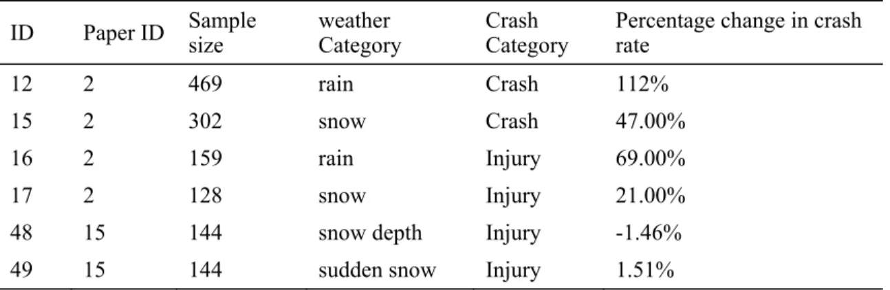
Coding: For each study that met the inclusion criteria, variables were coded into two tables. The general information table (see Table 4.1,) included document type, authors, publication year, country, study design, data source, and data on traffic volume. The study results information table (see Table 4.2.) included sample size, weather category (snow, rain, light snow, heavy snow, sudden snow, snow depth), weather specification, crash category (crashes, fatality, injury, property-damage-only), and percent change in crash rate. Table 4.1 and Table 4.2 show a few entries from the complete tables of this study to provide examples of these two table types.
Table 4.1 General information Paper
ID Author
Document
type Publication Date Study decade Country study method
2 Andrey Journal 2002 1990-1998 Canada Matched-pair
28 Table 4.2 Data information
ID Paper ID Sample size weather Category Crash Category Percentage change in crash rate
12 2 469 rain Crash 112%
15 2 302 snow Crash 47.00%
16 2 159 rain Injury 69.00%
17 2 128 snow Injury 21.00%
48 15 144 snow depth Injury -1.46%
49 15 144 sudden snow Injury 1.51%
Assessing study quality by validity score: As shown in Table 4.3., scores were assigned to each study on the basis that the validity of each study could be estimated by assigning a validity score in each of three categories: study design, traffic volume data, and level of aggregation. (e.g., as used by Elvik, 2001) The total validity score of a study is then the sum of these three scores. Validity classifications are shown in Table 4.3.
Table 4.3 Validity classification
Description Validity Score
Study design Matched-pair approach 2
Comparison study with certain controls 1
Traffic volume data
Hourly record from Automatic Traffic Recording (ATR)
stations 3
Averaged daily traffic data 2
Approximation from state-year vehicle miles traveled 1
Approximation from gasoline sale 1
Levels of Aggregation
Specified type of road 2
29
B. Comparison Studies with Percent Change as the Standard Measure
This study calculated an effect size d as the standard measure for each of the analyzed studies, specifically, the study used:
pooled M M sd Cohen σ 2 1
' = − (Hunter and Schmidt 1990). Eq. 4.1 where M1 and M2 are the means of the two populations being considered, and σpooled is a
function of the standard deviation of the two populations. To compute an effect size a parameter estimate and its standard error or variance estimation was needed. However, not all comparison studies consistently report those parameters. Thus as an alternative; percent change of crash rate (number of crashes per million vehicle miles traveled) to standardize outcome variables was selected.
For the comparison studies using relative crash risk ratio (Riski) as outcome variables, or for the studies providing crash rate (Ratei) during precipitation vs. non-precipitation conditions (Ratecontrol), percent change (Pi) was computed directly as shown in Eq. 4.2
and Eq. 4.3. 1 − = i i Risk P Eq. 4.2 control control i i Rate Rate Rate P = − Eq. 4.3
where i represents different adverse weather events.
For some of the regression studies, information has been extracted to compute the percent change in crash rate during adverse weather. These computations were based on the expert knowledge of weather conditions; a certain range of weather factor was selected in the x –axis and from this computed the corresponding crash rate change was computed.
Traffic Volume Deduction Correction
To ensure all the percent changes are comparable, it is necessary to correct those studies that did not control for the reduced traffic volume associated with adverse weather. For studies that used relative accident risk ratio (crash count ratio) as outcome variables or studies that did not take traffic volume reduction into consideration because
30
of the insufficient traffic volume data, the effect of reduced traffic volume on the crash rate was incorporated.
Two assumptions were made in order to do this correction as used in the study by Fridstrom et al. (2005):
• Exposure is proportional to traffic volume. This assumption is made because for a specified segment of road, the exposure measure vehicle miles traveled (VMT) is normally estimated by multiplying traffic volume on each road segment with the length of road segment and then summing them together to get an entire area VMT.
• Percent traffic volume reduction compare non-adverse weather condition can be defined asPvi. Though traffic volume reduction data are not available for each study, it is reasonable to assume that the estimations are similar from comparable literatures.
Doherty et al. (1998) suggested that during rain, traffic volume in Canada reduced 2% in comparison with non-precipitation days; this estimation is the same as a study conducted in London (Colding, 1974). Keay (2005) showed that the traffic volume decreased 1.35% to 2.11% on wet days in winter and spring, and can decrease up to 3.43% for heavier precipitation (2-10 mm). In terms of snow, traffic volume has a substantial reduction range from 7% to 56% (Hanbali, 1994) and 10% to 50% (Knapp et al., 2000). Knapp also estimated the average traffic volume reduction is 29% during heavy snow for interstate highways. Based on these studies, traffic volume reductions as shown Table 4.4 for a variety of precipitations were used.
Table 4.4 Traffic volume reductionPvi due to different weather conditions
Precipitation type light precipitation precipitation rain Light snow Snow heavy snow Percent deduction in
31
According to the these assumptions and Table 4.4, the percent change (Pi) of each study that needs traffic volume correction has been modified by Eq. 4.4 to provide the corrected percent change in crash rate (Picorrected).
( 1) 1 1 1 − + ∗ − = i vi corrected i P P P Eq. 4.4
Weight Each Study by Sample Size and Correct Sampling Error Variance
The occurrence of crashes is subject to random variation (Fridstrom et al, 1995). Thus studies with small sample size tend to have great variability and may lead to biased results. Computing the mean percent change across studies can reduce the impact of sampling error because of the large sample size obtained in this manner.
Because studies based on a large sample size would normally provide a better estimation, each study was weighed by its sample size. Also in many areas of scientific research, sampling error has been found to account for most of the observed variance, thus the sampling error variance was corrected by the Hunter-Schmidt method (Hunter and Schmidt, 2004).
Sample size (Ni), and the percent change in crash rate (Pi) during adverse weather event were available for each study. For each weather factor category, the mean percent change was computed as shown in Eq. 4.5.
∑
∑
= niPi ni
P / Eq. 4.5
The observed variance is given in Eq. 4.6 Variance =
∑
ni(Pi −P) /∑
ni2 Eq. 4.6
Thus, the sample-size-weighted mean was obtained and the sample-size-weighted variance of observed crash rate change for each weather factor was calculated. The formula for the sampling-error variance of proportions is shown in Eq. 4.7.
32
A sample-weighted mean of the sampling-error variance of proportions to be cumulated was then obtained as shown in Eq. 4.8.
Mean of Variance of Proportions =
∑
Pi*Qi/∑
ni Eq. 4.8Then sampling error variance was corrected by subtracting the sampling-error variance from the observed variance. This provided an estimate of the true variance plus variance due to other artifacts. Because of the lack of necessary information to allow for correction due to other artifacts, this estimation was used as an approximation for the true variance and was also used to compute the confidence interval.
C. Regression Studies Effect Size d and Percent Change as the Standard Measure The regression studies considered in this meta-analysis predicted the percent change in crash rate with a unit change in a certain weather factor. Most of the studies in this category applied Negative Binomial regression and provided sufficient information for effect size calculation. Thus effect size d (standardized mean different in crash rate) was applied to standardize each study result.
Effect Size
Normally effect size is the most reliable method to generalize studies. Effect size can be calculated in a number of different ways. Effect size d (Standardized mean difference) can be computed from a parameter estimate and its standard error or variance estimation, such as shown in Eq. 4.9. (Glass, 1981; Hunter and Schmidt, 1990). Note that this is the same as Eq. 4.1 above.
pooled M M sd Cohen σ1 2 ' = − Eq. 4.9 Or effect size d can also be computed from test statistics t, chi-square, or Z as shown in Eq. 4.10, Eq. 4.11 and Eq. 4.12 (Glass, 1981).
df t d 2 2 = Eq. 4.10
33 ) 1 ( ) 1 ( 2 2 2 χ χ − = N d Eq. 4.11 2 1 2 r r d − = , in which N Z r = Eq. 4.12
Depending on the information provided by each study, effect size d was appropriately calculated for each study. Then each effect size d was weighted by its sample size, and the sampling error variance was subtracted from the pooled variance. Finally the confidence interval was calculated and is presented for the pooled effect size d at the 95% level.
Percent Change
Percent change (Pi) here represents the percent crash rate change with per unit weather factor change. For Negative binomial regressions, it can be computed by reducing the exponential of the regression coefficient (Bi) of weather variables by 1.
D. Results
General Findings for Comparison Studies
A total of twenty nine comparison studies provided fifty three records, among which twenty four record crashes, eight record fatalities and seventeen record injuries. In addition four studies recorded property-damage-only crashes. Table 4.5 presents the estimated crash rate change during various weather conditions using 95% confidence intervals. Most of the percent changes were positive, indicating that during adverse weather conditions all types of crashes (fatality, injury, property-damage-only) exhibit some kind of increase in crash rate. Results also indicate that most precipitation events are associated with considerable increased crash risk, together with a somewhat lesser increase in injury risk and a minor increase in fatal crash risk. Generally, as the precipitation intensity increased, all levels of crash risk increased. High winds are also associated with an increase of the traffic crash rate.
34
Table 4.5 Crash rate change compare to non-adverse weather conditions.
Fatal Injury Crashes N Estimate (%) 95% C.I. (%) N Estimate(%) 95% C.I. (%) N Estimate(%) 95% C.I. (%) Snow 1 9 (9, 9) 4 75 (54, 96) 8 84 (68, 99) Rain 1 8 (8, 8) 7 49 (28, 70) 10 71 (31, 111) Wet pavement 3 384 (308, 459) \ \ \ 3 380 (249, 511) Heavy Snow \ \ \ 2 420 (350,490) \ \ \ Light snow \ \ \ \ \ \ 1 169 (169, 169) Heavy rain \ \ \ \ \ \ 1 93 (93, 93) High wind \ \ \ \ \ \ 1 100 (100, 100)
* Heavy snow: hourly precipitation intensity above 5 mm * Snow: total six hour precipitation amount above 2 mm * Light snow: total daily precipitation less than 25 mm * Rain: total six hour precipitation amount above 0.4 mm * High wind: wind speed above 15 mph
The “Wet Pavement Index” method was used in most of the studies that explored wet pavement related crashes. This method tends to overestimate the real crash risk (Brodsky and Hakkert, 1988). Also the “wet pavement” included in this analysis indicate all wet pavement events during winter months or cold temperature conditions, so the wet pavement actually represents various undesirable road surface conditions during the winter. As indicated in Table 4.5 above, on average the wet pavement conditions would increase both crash rate and fatal crash rate by over 300%. The estimated relative risk of crashes was increased on a slippery road surface without precipitation present, with an estimated injury risk of 1.70 (Andrey, 2003). A Swedish study showed the highest crash risk was associated with road slipperiness due to rain or sleet on a frozen road surface and the estimated increase of crash rate can be over 1000% (Norrman, 2000).