Growth and Poverty in Developing Countries
* Montek S. Ahluwalia, Nicholas G. Carter and Hollis B. CheneryDevelopment Policy Staff, The World Bank, Washington, DC 20433, USA Received December 1978
(from Journal of Development Economics 6 (1979) 299-341 © North-Holland Publishing Company)
Despite the developing countries’ impressive aggregate growth of the past 25 years, its benefits have only reached the poor to a very limned degree. Not only have the poorest countries grown relatively slowly, but growth processes are such that within most developing countries, the incomes of the poor increase much less than the average Although many policies have been proposed to counter these trends, little has been done to estimate the possibilities for significantly reducing world poverty within a reasonable period This paper develops a quantitative framework to project levels of poverty under different assumptions about GNP growth, population growth and changes in income distribution Although the interactions among development processes and policy instruments arc not modelled in any detail, the results serve to clarify the nature of the problem The policy simulations demonstrate that the elimination of absolute poverty by the end of this century is a highly unlikely prospect, even to achieve a substantial reduction will require a combination of policies designed to accelerate the growth of poor countries, to distribute the benefits of growth more equitably, and to reduce population increase.
1. Introduction
Although the output of the world economy has expanded at an unprecedented rate in the past quarter century, the benefits of growth have only reached the world's poor to a very limited degree. This is not due to any failure of developing countries as a group to share in the general economic expansion. Their income per capita rose by almost 3 percent per year over this period - considerably faster than in the past. The failure lies in the distributional pattern of past growth, which has left the poorest groups largely outside the sphere of economic expansion and material improvements.
There are two aspects to this phenomenon. First, the impressive growth record of the Third World as a whole conceals the fact that most of the poorest countries, containing the principal concentrations of the world's poor, have experienced lesser increases. Second, and equally important, there is mounting evidence that the growth processes under way in most developing countries are such that incomes of the poorer groups increase more slowly than the average.
International debate has centered around the design of policies to offset these trends. Proponents of a New International Economic Order consider the major objective to be the acceleration of growth in developing countries, with special concessions to the poorest among them. Others give greater weight to policies to improve the internal distribution of income, including direct measures to satisfy the basic needs of the poorest groups. These issues have been discussed so far in largely qualitative terms with little attempt to translate global targets for the eradication of poverty into more specific strategies whose feasibility can be examined.
The present paper suggests a quantitative framework for such an analysis and derives some preliminary conclusions from it.'Although there is not yet an adequate statistical basis for a formal analysis of the key relationships involved, there has been considerable progress in the past few years in several areas: (a) the definition and measurement of the incidence of poverty, using both physical and monetary indexes, (b) securing internationally comparable data on income levels, based on purchasing power comparisons, (c) measurement of the distribution of income and consumption within developing countries.
Our study is in three parts: (I) estimation of the extent of absolute poverty in developing countries and of the relationship between income distribution and rising levels of output (section 2). (II) analysis of past trends in growth and poverty in a representative group of
countries and of the implications of projecting these trends on the basis of present policies (section 3). (Ill) a consideration of possible improvements on this performance through acce-lerating income growth, improving its distribution and reducing fertility (section 4). We conclude with a comparison of alternative approaches to poverty reduction and their implications for national and international action. Despite the tentative nature of some of the underlying assumptions, it demonstrates that a combination of several approaches and of national and international action is more likely to succeed in reducing poverty than exclusive reliance on any one of them.
2. The dimensions of global poverty
This section attempts to evaluate the scale of poverty in the developing world and the available evidence on the effect of growth on poverty. The analysis is based on a sample of 36 countries which are listed below in table 1. The sample is broadly representative of developing countries with mixed or market-oriented economies. They span the wide range of income levels observed in the developing world and reflect ils distribution by broad geographic regions. Together, the countries in our sample account for about 80 percent of the population of the developing world, excluding China.1
2.1 Defining absolute poverty
The First step in measuring the scale of poverty is to establish a common poverty line to be applied across countries. It is self-evident that such a definition is necessarily arbitrary. Attempts to define absolute poverty in terms of some objectively determinate minimum level of consumption that is necessary for continued survival' do not escape this problem, since the notion of continued survival is undefined. Ai the very least we would need to specify survival through some given life expectancy in a given environment. Present levels of life expectancy in most developing countries are quite low and do not provide a basis for defining minimum requirements. Increases in life expectancy will require higher levels of real consumption including not only better food intake, but also a better general environment for health and nutrition.
Not only is the notion of a biologically determined absolute poverty level imprecise, it is in any case wrong to think that poverty should be defined solely in terms of biological requirements. Ultimately, concepts such as poverty lines are operationally meaningful only when they acquire some social reality, (hat is, when there exists a sufficient social concensus that a particular level of living represents an objective which claims a high social priority. Once we recognize that acceptability by contemporary social standards is a key requirement, it follows that poverty lines used in national policy debates will vary across countries, reflecting differences in levels of economic, social and political development. By the same token, they will also change over time.
For these reasons any effort to define a poverty line to be applied across countries and over lime must be approached with caution. We have concluded, however, that with all its limitations such a measure can provide a useful basis for international policy. For this purpose, it is less important that the poverty line correspond to some objective criteria for minimal levels than that the absolute level chosen be conservative and roughly comparable across countries. In this paper we have based our definition on the poverty lines which have been used in India, which is the largest and one of the best studied developing countries.
1
The principal limitation on the size of the sample is the availability of data on income distribution. Indeed, of the 36 countries in our sample, fairly reliable distribution data were available only for 25. For the remainder we have used estimates of the distribution of income based upon cross country comparisons (sec appendix table I). We have resorted to this procedure only in cases where inclusion of the country was very desirable either because of its size or to ensure adequate geographical representation.
Table 1
Simple panel: Per capita income, population and poverty. a
1975 GNP per capita c Percentage of population in poverty in 1975 Country b at official exchange rates using Kravis adjustment factors Population 1975 (millions) using Kravis adjustment factor using official exchange rates Group 4 (under $350 ICP)
(1) Bangladesh 72 200 80.7 64 60 (2) Ethiopia 81 213 27.3 68 62 (3) Burma 88 237 30.9 65 56 (4) Indonesia 90 280 130.0 59 62 (5) Uganda 115 280 11.5 55 45 (6) Zaire 105 281 20.6 53 49 (7) Sudan 112 281 18.1 54 47 (8) Tanzania 118 297 14.8 51 46 (9) Pakistan 121 299 73.0 43 34 (10) India 102 300 599.4 46 Subtotal 99 284 1006.3 51 49 Group B ($350-$750) (11) Kenya 161 413 13.4 55 48 (12) Nigeria 176 433 75.3 35 27 (13) Philippines 182 469 41.5 33 29 (14) Sri Lanka 185 471 14.1 14 10 (15) Senegal 227 550 4.3 35 29 (16) Egypt 238 561 37.2 20 14 (17) Thailand 237 584 41.6 32 23 (18) Ghana 255 628 9.8 25 19 (19) Morocco 266 643 17.3 26 16 (20) Ivory Coast 325 695 5.9 25 14 Subtotal 209 511 261.4 31 24
Group C (greater than $750)
(21) Korea 325 797 34.1 8 6 (22) Chile 386 798 10.6 11 9 (23) Zambia 363 798 4.9 10 7 (24) Columbia 352 851 24.8 19 14 (25) Turkey 379 914 39.7 14 11 (26) Tunisia 425 992 5.7 10 9 (27) Malaysia 471 1006 12.2 12 8 (28) Taiwan 499 1075 16 1 5 4 (29) Guatemala 497 1128 5.5 10 9 (30) Brazil 509 1136 106.8 IS 8 3
1975 GNP per capita c Percentage of population in poverty in 1975 Country b at official exchange rates using Kravis adjustment factors Population 1975 (millions) using Kravis adjustment factor using official exchange rates (31) Peru 503 1183 15.3 18 15 (32) Iran 572 1257 33.9 13 8 (33) Mexico 758 1429 59.6 14 10 (34) Yugoslavia 828 1701 21.3 5 4 (35) Argentina 1097 2094 24.9 S 3 (36) Venezuela 1288 2286 12.2 9 5 Subtotal 577 1220 427.6 13 8 Total 237 555 1695.3 38 35
a Sources: GNP and population from World Bank Data Bank. Kravis adjustment factors
from Kravis, Heston and Summers (1978a).
b Countries ordered by 1975 GNP per capita adjusted by Kravis factor. c In 1970 US $.
There is an extensive literature on the measurement of poverty in India and a variety of poverty lines have been proposed, some of which have received official sanction. The most widely used poverty line is defined by the total consumption expenditure needed to ensure a daily supply of 2250 calories per person, given the observed expenditure patterns of the Indian population.2 Estimates of the extent of poverty in terms of this standard vary from year to year, but most estimates range between 40 and 50 percent of the total population. For our study we have adopted an intermediate position, setting the poverty level to be applied across countries as the income per head accruing to the forty-fifth percentile (approximately! of the Indian population. Application of this essentially South Asian standard across all developing countries yields estimates of poverty that arc conservative in the sense of understating the extent of the problem by standards appropriate for richer countries.
Having chosen a poverty line, the next step is lo apply it in such a way as to ensure comparability across countries. The use of official exchange rates to define equivalent levels of expenditure in different countries does not ensure equivalent levels of real purchasing power. We have attempted to overcome this problem by using 'equivalent purchasing power conversion ratios' estimated by Kravis and associates from data collected by the United Nations International Comparison Project (ICP).3 Using these ratios, we can convert the per capita GNP levels in each country into GNP per capita measured in dollars of 1970 U.S. prices hereafter called ICP dollars. The resulting estimates are shown in table I. Our poverty line is easily calculated given the income distribution for India for 1975 and its estimated level of per capita GNP in ICP dollars. We have chosen a poverty line of 200 ICP dollars -
2
It should be emphasized that poverty lines defined in terms of consumption expenditure ignore the fact that there is very considerable variation in caloric intake achieved at any given level of expenditure. In any case, the underlying specification of a tingle caloric norm is itself questionable. Nutritionists have shown that there is very considerable variation in caloric requirements even for the same individual over time.
3
The International Comparison Project has been a joint responsibility of the United Nations Statistical Office, the World Bank, and the International Comparison I nil of the University of Pennsylvania. Two volumes of results have been published; see Kravis, Kenesscy, Heston and Summers (1975), which includes detailed estimates for India, and Kravis. Heston and Summers (1978a). The conversion factors used here were estimated by Kravis, Heston and Summers (1978b). These ratios are called 'Kravis factors' in this paper; the resulting unit of value is identified as an ICP dollar. Other methods of estimating conversion factors from the ICP data are under study.
the level of the 46th percentile which is then applied to the income distribution and per capita GNP data for other countries to estimate the extent of poverty in each case.4
This income-based approach to defining poverty makes no explicit allowance for the achievement of minimum levels for essential public services such as health, education, access to clean water and sanitation. These are fundamental elements in a more complete definition of poverty that are of crucial importance in designing a balanced program of poverty alleviation. but they remain outside the present analysis.
2.2. The extent of poverty in developing countries
The procedure just described enables us to estimate the extent of poverty in each country using an income level that reflects comparable levels of purchasing power. These estimates are reported in the fourth column of table 1. For purposes of comparison, we have also estimated the extent of poverty in our sample without the conversion ratios. In this case, we measure per capita GNP for each country in US dollars by converting at official exchange rates, calculate the income level of the 46th percentile in India and apply this level to the data for all other countries. These estimates arc shown in the last column of table 1. Since in each case the poverty line is based on the income of the same percentile of the Indian population, the difference between the two estimates lies in the extent to which poverty in other countries is altered relative to India.
In general, we find that the use of purchasing power ratios reduces the differences between the incidence of poverty in middle and higher income countries compared to the low income countries. The use of ICP dollars also raises the estimates of poverty relative to India in the low income countries. This rise reflects the fact that the Kravis purchasing power ratios suggest that GNP levels in both groups of countries are overstated relative to India.5
The major features of global poverty as revealed in the estimates based on purchasing power ratios correspond broadly to other estimates.6 Almost 40 percent of the population of the developing countries live in absolute poverty defined in terms of income levels that are insufficient to provide adequate nutrition by South Asian standards. The bulk of the poor are in the poorest countries: in South Asia, Indonesia, and sub-Saharan Africa. These countries account for two-thirds of the total population and well over three-fourths of the population in poverty. The incidence of poverty is 60 percent or more in countries having the lowest levels of real GNP.
Although the incidence of poverty is much lower for the middle income developing countries in our sample, our estimates of poverty in this group of countries increases from 24 to 31 percent when purchasing power ratios are used to estimate GNP. There is a similar increase in the high income group from 8 to 13 percent.
4
Although the Indian estimates of poverty arc based on a consumption standard applied to the distribution of population across consumption levels, in our study we have defined the poverty line by the income per head observed at the forty-sixth percentile of the Indian population The use of per capita GNP instead of per capita personal income (which is clearly more appropriate) is dictated by the absence of data on the personal income component of GNP Since the proportion of personal income in GNP declines at higher levels of development, our procedure probably understates the extent of poverty.
5
Although the use of the Kravis conversion ratios is clearly a step in the right direction, it also raises questions that we have not addressed for example, it is likely that the purchasing power ratios vary for different income groups within a country Since an important element underlying this correction is the relative undervaluation of services in low income countries, and since services arc disproportionately consumed by the rich, it may he that official exchange rates understate incomes of the rich more than of the poor. By applying a single average correction factor to GNP per capita we ignore this problem. A similar argument can be made for distinguishing between conversion rates relevant for different regions or for urban and rural areas.
6
See, for example. Chenery, Ahluwalia, Bell, Duloy and Jolly (1974, ch.1). 5
It is interesting to compare our estimates of absolute poverty to those reported for selected Latin American countries in a recent joint study by the Economic Commission for Latin America and the World Bank.7 This study estimates a much higher incidence of poverty in Latin America around 40 percent for the region as a whole but this results from the adoption of poverty lines that are significantly higher than those derived from South Asia. For example, the food budget was geared to a higher minimum nutritional level and was constrained to ensure some minimum consumption of higher value foods (meat, fruit, eggs and milk).8 The food budget thus obtained was used to define two different poverty lines: a destitution line", defined as income equal to the food budget, and a “poverty line”, defined as income equal to twice the food budget to allow for non-food expenditures. Estimates of the extent of poverty in the Latin American countries in our sample are broadly in line with Altimir's estimates of the extent of destitution (about 19 percent of the population of Latin America). Furthermore, projections using either method show little prospective decline in absolute poverty with present trends.
2.3. Poverty and growth: A review of evidence
The extent of poverty in any country depends upon two factors - the average level of income and the degree of inequality in its distribution. Although the estimates of income growth are relatively good, we have little reliable information on how the distribution of income has changed over time. Systematic time series data based on reliable sources and using comparable concepts are simply not available. At most there is a handful of countries for which we have observations for 2 or more years spanning a decade or so.
In the absence of time series data for individual countries any assessment of changes in the distribution of income accompanying development in the past must be based on what can be inferred from cross-country data. This evidence has been extensively studied in recent years and a brief summary of the findings is presented below.
The central theme in the continuing debate on trends in income distribution is whether development in the past has been accompanied by such an increase in inequality that the poor have benefited relatively little from overall growth. Much of this debate has its origin in the classical contributions of Kuznets (1955, 1963), who hypothesized that the process of development was likely to be accompanied by a substantial increase in inequality, which would reverse itself only at a relatively advanced stage. Kuznets’ original speculation was based on fragmentary historical data for the now developed countries, but in its later development, especially at the hands of subsequent contributors, the investigation of this hypothesis has relied almost entirely upon crosscountry evidence. A number of studies -Adelman and Morris (1973), Paukert (1973), Chenery and Syrquin (1975) and Ahluwalia (1976) - using different, and progressively more reliable sets of cross-country data, have reported confirmation of the hypothesis to some degree.9 The average pattern discerned in the data is one of significant increase in inequality as income levels rise from the least developed to about US S600 per capita in 1975 prices.10
The extent of the increase in relative inequality reported by different authors varies substantially. At one extreme, Adelman and Morns (1973) have argued that the cross-country data suggest that economic growth will be accompanied by a process of prolonged
7
See Altimir (1979). 8
The calorie requirement used is also higher ranging between 2260 and 2350 calories per person per day and there is also a specified minimum protein requirement varying between 40 to 43 grams per person. Furthermore, the food budgets were calculated so as to provide explicit allowance for a minimum consumption of vegetables and fruit to provide minerals and vitamins in a balanced diet.
9
It must be emphasized that given the limitations of cross-country data, this evidence is al best persuasive. For a skeptical view see Papanek (1978).
10
For the typical developing country, $600 in 197$ prices and at official exchange rates is approximately equal to 800 IC°P dollars al 1970 prices This is the estimated turning point for the share of the lowest 60 percent. As noted by Ahluwalia (1976) the turning point for the lower 40 percent and the lowest 20 percent occurs at successively higher levels of per capita GNP.
absolute impoverishment for large sections of the population. Others, such as Ahluwalia (1976), have argued that although the cross-country evidence points to increasing inequality in the early stages, this does not completely offset the effect of growth. Income levels of the poorer quintiles are likely to rise, but much more slowly than the average.
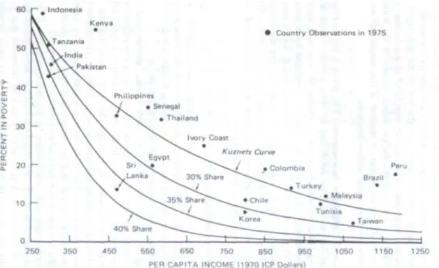
Fig. 1. The Kuznets curve with country observation.
The limited time series evidence provides some support for Ahluwalia’s conclusion. There are a number of countries for which estimates arc available of the distribution of income (or consumption) at two points in time spanning about 10 years in each case. While many of these countries appear to show some decline in the shares of the poorer quintiles over lime, in no case is this decline in shares sufficiently sleep to offset the recorded growth in mean incomes.11 Some of this evidence is discussed below.
A simplified representation of the Kuznets effect is given in fig. 1, which plots the per capita income of the top 40 percent of the population against that of the bottom 60 percent. Lines of constant per capita income appear as downward sloping straight lines. Ahluwalia's estimate of the Kuznets curve in these dimensions appears as a curve with maximum inequality in the vicinity of 800 ICP dollars (1970 prices) Between the income levels of 200 and 800 dollars the share of the lower 60 percent declines from 32 percent to 23 percent of the national income. A country that followed this average relation would have about 80 percent of the
11
It should he noted that here we are referring lo changes over time for (he economy as a whole. This does not rule out the possibility of increased impoverishment in a pan of the economy, e.g. the rural areas in general, or a particularly depressed region. See for example. Griffin and Khan (1978) for an exposition of the view that growth has been accompanied by increasing rural poverty.
increment accruing to the upper 40 percent of its citizens and quite modest increases for (he remaining groups.12
This average relationship can be compared with the observed movement of individual countries over specified periods of time, as shown by the arrows in fig. 1. These observations relate to a relatively short time period typically 10 years - and the data are often not strictly comparable for a given country. Nevertheless, the broad picture of intertemporal movements is generally consistent with the average cross-country path indicated by the Kuznets curve. The underlying observations for each country do not show any case of a decline in the per capita income of the lowest quintile.
It is important to emphasize that the average cross-country relationship should not be interpreted as an iron law. Individual countries that are able to establish the preconditions for a more egalitarian distribution of income and to stimulate growth in such a policy environment, as illustrated by Yugoslavia, Taiwan and Korea, may well be able to avoid or moderate the phase of increasing inequality. But there are a number of reasons why such a pattern is likely to emerge with a continuation of past policies, especially in the non-socialist countries characterized by sharp inequalities in the initial distribution of productive wealth (including land). For one thing, development typically involves a shift of population from the low income, slower growing agricultural sector to the high income, faster growing modern sector. This process, which is central to the dual economy theories of Lewis (1954) and Fei and Ranis (1964), can be shown to generate a phase of widening inequality.13 This is especially true when the growth of the modern sector takes an increasingly capital intensive form, as in Mexico and Brazil, with incomes per person employed rising relatively rapidly but with a limited increase in employment. It is less true of the more labor intensive form, illustrated by Taiwan and Korea, which is characterized by high rates of absorption of labor and a more rapid approach to full employment. Policy clearly has an important role in determining which form predominates.
There are several other factors that contribute to widening inequality. Economic growth is likely to produce a more rapid rise in the demand for skilled labor compared to unskilled labor, leading to widening inequality in the early stages, when the supply of skilled labor expands relatively slowly. These disequalizing factors are often exacerbated by an institutional and policy framework that is biased in favor of the modern, urban sectors of the economy, leading to an excessive flow of resources to these sectors, and increasing the incentives for capital intensive production.
Combining the available evidence with these a priori considerations, we conclude that the most likely outcome associated with economic growth in poor countries is some increase in inequality. The projections discussed below adopt this assumption in the Base Case but depart from it in considering the effects of improved distributional policies.
The use of the Kuznets curve in projections also implies that the distribution of income will improve in countries with a per capita income above 800 ICP dollars without specifying the effort required to redirect government policies. Needless to say, we cannot assume that this improvement will take place automatically. The low inequality observed in the developed countries today is as much the result-of institutional evolution resulting from particular historical and political factors as of their level of development. It has been argued by Bacha (1977) that the observed reduction in inequality in the developed countries over the first half of this century arose from social and political changes following the first world war that are
12
Ahluwalia’s (1976) estimates from which these aggregate measures are derived were made for quintiles, which show that most of the change in shares is concentrated in the upper 20 percent and lower 40 percent of the population Further details are given in the technical appendix.
13
See Robinson (1976) and Ahluwalia (1976), Bell (1979) gives a more formal demonstration of the possibility of U-shaped curves relating to the wage share in simple dual economy models.
not likely to be replicated in countries approaching industrial maturity today.14 We note that of the countries in Group C of table 1, all of which are past the turning point estimated from cross-country data, only Taiwan shows some evidence of experiencing the second phase of the Kuznets curve.
However, although our projections may be overoptimistic about future developments in countries approaching industrial maturity, this assumption does not affect our projections of global poverty.
3. Consequences of existing policies
Our analysis focusses upon three aspects of development in each country in our sample: (a) the growth of aggregate income, (b) the growth of population, and (c) changes in the distribution of income by deciles. These measures can be combined to analyze the evolution of relative and absolute poverty over time for individual countries or groups of countries. 3.1. The base projection
The conceptual basis for our analysis is a disaggregation of income growth in each country into a separate growth pattern for each income class (decile), expressed in ICP dollars of constant purchasing power. When applied to our sample of 36 countries, this procedure yields a time series of per capita income for 360 population units. These can be aggregated to determine the numbers of people below a given poverty line in groups of countries as well as measures of relative inequality within groups. This procedure will be applied both in analyzing past trends in individual countries and in determining the distributional consequences of projected growth.
Despite the variable quality of the data on income distribution, it is useful to retain individual countries as units of observation, both because of the substantial difference in their initial conditions and the necessity of defining the scope for policy changes on a country basis. The analysis focusses on the results for groups of countries, since aggregation reduces the effects of errors in country data.
The procedure indicated above is carried out in four steps:
a) estimation of the income level of each country (Ytj) for the past (1960-1975) and
projection of this level for the future (1975 2000).
b) estimation of population (Ntj) by country for the same periods,
c) estimation of income shares by deciles (Dtij) for each country and hence the level of
income for each decile group,
d) determination of the number of people (Ntj) below the absolute poverty line in each
year.
The results of step (c) can be used to compute measures of inequality for any country or group of countries.
Growth in income and population. The present study was designed to determine the distributional consequences of existing country projections of GNP and population. These have been made by the World Bank in the context of a global analysis of international trade and capital flows. They provide a point of departure (Base Case) from which to consider changes in internal and external policies. The Base Case incorporates changes in GNP
14
The most important of these developments was the strengthening of organized labor following the first world war and its subsequent political role in developing a welfare state However, this argument should not be overstated, since these institutional changes were themselves based on an underlying economic transformation in the role of labor arising from the phenomenon of labor scarcity and the greater role of human skills in the production process. Similar processes can be expected to occur in the future, although in different social and political contexts, and they are likely to strengthen tendencies towards greater equality, although perhaps not so soon as predicted by the cross-country estimates.
growth expected to occur with some improvement in existing policies as well as changes in population growth that can be anticipated from existing demographic trends. Table 2 gives the growth in population and GNP determined on this basis for the period 1975 2000.15
Table 2.
Sample panel: Indices of growth and distribution. a GNP growth rates Population growth rates Share of lowest 40 percent Number of people in poverty (millions) b 1960- 1975 1975-2000 1960-1975 1975- 2000 1975 estimate Base Case projec tion 2000 1975 estimat e Base Case projecti on 2000 Group A (under $350 ICP)
(1) Bangladesh 2.4 4.6 2.7 2.5 20.1 17.4 52 56 (2) Ethiopia 4.3 4.1 2.1 2.6 16.8 15.0 19 25 (3) Burma 3.2 2.5 2.2 11 15.7 15.2 20 29 (4) Indonesia 5.2 5.5 2.1 1.7 16.1 11.7 76 30 (5) Uganda 4.0 3.2 2.9 2.8 14.4 14.0 6 12 (6) Zaire 4.3 4.8 2.6 17 14.6 12.7 11 13 (7) Sudan 3.0 6.0 2.8 18 14.5 12.0 10 8 (8) Tanzania 6.8 5.4 2.9 19 143 12.3 8 9 (9) Pakistan 5.6 5.2 3.2 17 16.5 14.5 32 26 (10) India 3.6 4 5 2.3 1.9 17.0 14.6 277 167 Subtotal 3.8 4.7 2.4 11 16.7 13.9 510 375 Group B ($350-$750) (11) Kenya 7.0 5.9 3.2 3.5 8.9 7.7 7 11 (12) Nigeria 7.1 5.2 2.6 19 13.0 11.8 27 30 (13) Philippines 5.6 7.3 3.0 14 11.6 10.3 14 6 (14) Sri Lanka 4.2 3.8 2.4 1.7 19.3 18.2 2 2 (15) Senegal 1.5 4.0 2.1 14 9.6 8.9 1 2 (16) Egypt 4.2 6.1 2.5 1.8 13.9 13.5 7 5 (17) Thailand 7.5 6.7 3.0 2.4 115 10.9 13 4 (18) Ghana 2.7 2.1 2.6 2.9 11.2 11.9 2 6 (19) Morocco 4.4 6.2 2.7 18 13.3 10.9 4 2 (20) Ivory Coast 7.7 5.8 33 2.9 10.4 10.4 1 1 Subtotal 5.5 5.8 2.7 2.6 12.0 10.0 81 70 Group C (above $750) (21) Korea 9.3 8.1 2.1 1.6 16.9 19.1 3 1 (22) Chile 2.3 6.0 2.2 1.5 13.1 14.3 1 1 (23) Zambia 3.4 4.9 2.9 3.3 13.0 12.9 0 1
15
The growth rate are based on projections lo 1985 or 1990 that underlie recent World Bank studies of the world economy (1977, 1979) They lie between the Base Case projection for 1980 lo 1990 of the latter (5.6 percent) and the more optimistic projection (6.6 percent).
GNP growth rates Population growth rates Share of lowest 40 percent Number of people in poverty (millions) b 1960- 1975 1975-2000 1960-1975 1975- 2000 1975 estimate Base Case projec tion 2000 1975 estimat e Base Case projecti on 2000 (24) Colombia 5.6 7.4 3.1 1.8 9.9 11.5 5 2 (25) Turkey 6.4 6.3 2.2 1.1 9.3 10.4 6 4 (26) Tunisia 6.1 7.5 2.5 1.9 11.1 13.3 1 0 (27) Malaysia 6.7 6.7 2.8 1.8 11.1 13.3 1 1 (28) Taiwan 9.1 6.2 2.8 1.7 22.3 24.4 1 0 (29) Guatemala 6.1 6.0 2.5 1.7 11.3 12.4 1 1 (30) Brazil 7.2 7.9 2.9 2.6 9.1 11.9 16 7 (31) Peru 5.7 6.3 2.8 2.5 7.3 8.8 3 2 (32) Iran 9.5 7.2 3.1 2.4 8.2 11.0 5 2 (33) Mexico 6.8 6.8 3.4 3.0 8.2 10.8 8 6 (34) Yugoslavia 5.8 6.1 1.0 0.7 18.8 23.9 1 0 (35) Argentina 4.0 4.5 1.5 1.0 15.1 18.5 1 1 (36) Venezuela 5.8 6.8 3.5 2.9 8.5 12.9 1 1 Subtotal 6.4 6.9 2.6 2.2 9.9 10.0 54 30 Total 5.4 6.2 2.5 2.2 9.8 6.5 644 475 a
Source: GDP growth from Prospects for Developing Countries, 1978 1985; World Bank (1977). b
Totals may not add due to rounding.
Since our main concern is with the incidence of poverty, the assumptions made for the poorer countries are more important than those for the rest of the panel. In the past the economies of the poorer countries have grown more slowly because of the greater weight of the agricultural sector (whose growth is limited by both demand and technology), lower rates of savings, and other structural factors. In addition, the international environment has been somewhat less favorable to the growth of poor countries and domestic policy failures have probably been more pronounced.16
For the future some acceleration of growth is anticipated in several of the largest poor countries India. Indonesia and Bangladesh so that the average of the group is expected to increase from 3.7 percent to 5.0 percent. This income growth will be partially offset by an increase in population growth as death rates fall more rapidly than birth rates. Although only a limited acceleration of aggregate growth is projected for the other developing countries, this will be augmented by a fall in population growth as they move further into the demographic transition.
Changes in distribution. The specification of plausible changes in distribution raises two main issues. If existing policies continue, what changes in distribution can be expected as a result of the growth processes now under way? Conversely, if a government takes stronger measures to improve income distribution, what is likely to happen to growth? Although there is no consensus among economists on either of these questions, we will make the following assumptions for the present analysis.
16The relation between growth and income level is analyzed by Robinson (1971) and Chenery,
Elkington and Sims (1970). Chenery and Carter (1973) give an evaluation of the effects of internal and external factors on past growth for a sample of countries similar to the present one.
In the first place, since time series data will not support a separate analysis of each country, we initially assume average behavior for countries having a given initial income level and distribution. More specifically, we assume that the cross-section estimates of the Kuznets relation discussed above are representative of the behavior of mixed economies over time in the absence of effective government action to alter them. This leads to a worsening of income distribution for countries below a per capita income of 800 ICP dollars. We also assume that there is a tendency for the income distribution to improve above this level, although the historical causes of this improvement have been as much political as economic.
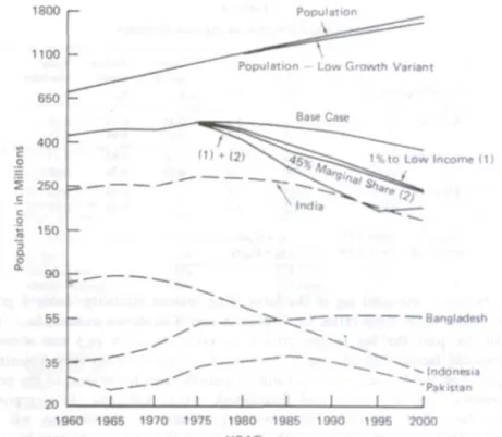
Fig. 2. Alternative simulations 1975-2000.
To translate these assumptions into a projection procedure, we construct a separate Kuznets curve for each country by means of which the distribution estimated for 1975 (or any other year) can be projected to higher or lower levels of income.17 The country-specific curves differ in their starting points but have the same curvature. The effect for representative countries above or below the average distribution is shown by the solid lines in fig. 2. The Base Case projection for a country such as India, which is close to the average to start with, would follow (he Ku/nets curve quite closely. Other countries, such as Brazil or Korea, retain their relative positions above or below the average distribution and in this sense are assumed to run ‘parallel’ to the Kuznets curve.18 Although this is a highly stylized
17The formula for this function assumes that the two parameters in the quadratic function describing
the Kuznets curve apply to each country, as indicated in the appendix. 18
The actual projection! axe made fur each decile and are aggregated here to illustrate the overall effects.
interpretation of the existing evidence, it is more plausible than assuming that there is no effect of economic development and industrialization on distribution, which is the only obvious alternative.19
The question of the effect of changing distribution on growth arises later when we take up alternative distributional policies. We then assume that there is a reduction in growth proportional to the fall in the share of income (and savings) of the upper income group. The effects of this assumption are illustrated by the second set of projections in fig. 2, which arc discussed below.
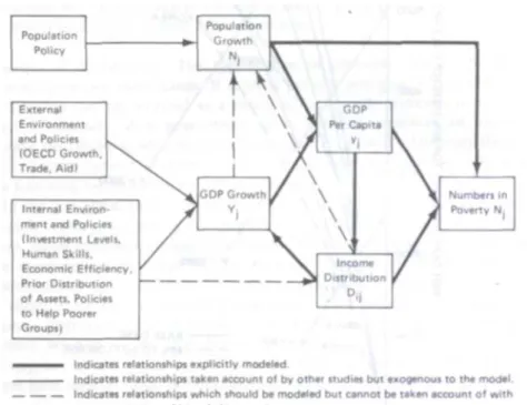
By way of summary, the relations among the several determinants of poverty are shown schematically in fig. 3. The links between internal and external policies and the extent of poverty in each country are traced through three intermediate variables: population (N), per capita GDP (y), and income distribution (D). Projections of population growth and GDP are taken from other studies and become exogenous variables in the Base Case. The distribution of income by decile (Dij) is generated as a function of the initial distribution and
the average variation with per capita income.
Fig. 3. Schema lie representation of causal relationships underlying simulation models. In the Base Case simulation there is no feedback from the distribution of income to the rate of growth. However, in simulations where we depart from the distributional behavior of the Base Case we allow for a feedback from income distribution to GDP growth. Other possible feedbacks, such as those from GDP and its distribution lo population growth, are not analyzed explicitly and are indicated by dashed lines. (A mathematical statement of the simulation model is given in the appendix.)
3.2. Trends in inequality and poverty
The basic projections are given in table 3 for the three country groups and for the poorest 40 percent of the people in each group. The trends for the period 1960 1975 are simulated in the same way for purposes of comparison. These results bring out the main links between overall growth and the changes in inequality and absolute poverty.
19
We have, however, made calculations bawd on the latter assumption in order to show the net effect of the Kuznets hypothesis. See Chenery and Carter (1977).
Table 3. Growth and poverty in developing countries. Projections for 2000 1960 estimates 1975 a Historical trend Base Case* (I) Per capita income (PCY) (ICP $ 1970 prices)
All LDCs 367 555 (2.8) 1446(3 9) 1462 (4.0)
Low income 233 284 (1.3) 464 (2.0) 536 (2.6)
Middle income 337 511 (2.8) 1179 (3.4) 1189(3.4)
High income 714 1220(3.6) 3829 (4.7) 3724 (4.6)
(II) PCY lowest 40 percent UCP S 1970 prices)
All LDCs 109 136 (1.5) 205 (1.7) 236 (2.2)
Low income 102 118 110) 159 (1.2) 186 (1.8)
Middle income 104 153 (2.6) 300 (2.7) 288 (16)
High income 174 301 (3.7) 961 (4.8) 1114 (5.4)
(III) Income shares lowest 40 per cent [percentages)
All LDCs 11.9 9.8 5.7 6.4
Low income 17.5 16.7 13.7 13.9
Middle income 12.4 12.0 10.1 9.7
High income 9.7 9.9 10.0 12.0
(IV) Number of poor (millions)
All LDCs 597 644 589 475
Low income 438 510 493 375
Middle income 86 81 56 70
High income 72 34 40 30
(V) Percentage of population in poverty
All LDCs 50.9 38.0 20.2 16.3
Low income 61.7 50.7 29.5 22.4
Middle income 49.2 31.0 11.4 14.2
High income 24.9 12.6 5.4 4.0
a Figures in parentheses are annual growth rates between 1960 . b
Figures in parentheses are annual growth rates between 1975 and 2000.
c Growth rates as in ‘Prospects for Developing Countries’, World Bank, 1977.
ηpa measures the total lag in the form of an income elasticity. Table 3 gives the measures for
these ratios for Groups A and B as shown in table 3a.
Inequality. The sources of growing inequality in the developing world as a whole can be summarized by means of the Theil index, which permits a decomposition of inequality into two elements: within and among countries.20 This index and the proportion due to inequality among countries are shown below for past and future periods:
1960 1975 2000
Theil index 0.57 0.67 0.77
Proportion due to variation among countries (%) 32 37 50
20
The Theil index is defined as Σyi, In (yi / ni), where yi, and ni, are the iharet of income and population of a given decile unit in the total income or population of the group of countries. This index varies between 0 in the case where all income shares are equal lo population shares, and log l/ nj, where nj is the population share of the smallest group. Note that inequality ii at a maximum when all income accrues to the smallest possible group.
There is a substantial increase in overall inequality and in the proportion due to variation among countries. This increase in inequality can be examined in terms of the interaction of two factors, (a) the intercountry lag between the countries of Group A and all developing countries, (b) the within-group lag in the growth of the poor within these countries in relation to the average. Thus, the growth of income of the poorest 40 percent in Group A countries (who account for about 80 percent of the world's poor in our base year) can be written as
, G G G G G G G pa a pa a pa = ⋅ ⋅ =
η
where Gpa is the growth of income of the poorest 40 percent in Group A, Ga is the growth of
Group A, G is the growth of all developing countries and Table 3a
Growth lags within and among country Groups. Country group Gpi Gi Inter-group
Within-group Total elasticity A. Low I 1.0 1.3 0.46 0.77 0.35 II 1.8 2.6 0.65 0.69 0.45 B. Middle I 2.6 2.8 1.00 0.93 0.93 II 2.6 3.4 0.85 0.76 0.65 Total I 1.5 2.8 0.54 0.54 II 2.2 4.0 0.55 0.55 Period I: 1960-1975 ηI = Gi /G Period II: 1975-2000 ηp= Gpi /Gi
In the past the lag in the growth of poor countries (ηa) was a more important factor than the
lag in growth of the poor within these countries (ηp).21 For the future, we project higher
growth rates for several of the poor countries notably India and Bangladesh that will raise the intergroup ratio from 0.46 to 0.65. The worsening of internal distribution will be accentuated by more rapid growth, however, so that the two factors become of roughly equal importance in explaining the projected lag in the income growth of the poor (0.45). For the middle income group, on the other hand, both lags are projected to increase. As a result no improvement in the total elasticity (0.55) is projected for developing countries as a group with existing policies.
Poverty. The lag in the growth of income of the poorest 40 percent in low income countries is obviously at the core of the problem of world poverty. Trends in absolute poverty are shown in (he last two sections of table 3 and in fig. 4 below. In 1975 the numbers of the poor were still increasing in almost all of the countries in Group A but had started lo decline in most countries in Groups B and C. For the future a continued rise is projected in a number of the poor countries, but it is offset by a reversal of this trend in Indonesia, India and Pakistan. The net effect is a decline in absolute poverty of around 10 percent in the low and middle groups and considerably more in Group C.22
21
If the two factors were measured for individual countries rather than for Group A as a whole, the difference would be even greater.
22
The less optimistic projection in table 3, based on historical trends in each country, shows only a modest reduction in poverty in 2000 to the level existing in 1960.
Fig. 4. Poverty profile (Group A countries only): 1960-2000.
In overall terms the number of absolute poor in all developing countries (except for the centrally planned economics) would be on the order of 600 million people in the year 2000 when allowance is made for countries omitted from our sample. This Figure defines the magnitude of the problem to be addressed in devising policies that will lead to a more rapid reduction in poverty. Although in relative terms these projections represent impressive progress in reducing poverty from about 50 percent of the population of developing countries in 1960 to 16 percent in 2000 they fall considerably short of the results that might be achieved with more effective policies.
3.3. Variation in country experience
Although we have usable time series data for only twelve countries, they include a considerable variety of experience with both growth and distribution. Table 4 contains the statistical data underlying the graphical analysis of these countries in fig. 1. This table also shows the growth rate of per capita income of the lower 60 percent and its relation to the country average (ηp).
The countries in table 4 have been classified into three groups on the basis of two criteria, the income share of the lower 60 percent in the latest year and the share of the increase in income going to this group over the period. The five countries in Group (I) have a terminal share ranging from 28 to 39 percent and incremental shares above 30 percent. At the other extreme, the three countries in Group (III) have terminal shares in the range of 18 to 21 percent and incremental shares of only 16 to 18 percent. Distribution in the former group is considerably better than (he Kuznets curve in fig. 1 and in the latter group considerably worse. The four countries in Group (II) are close to the average relation.
In order to determine the scope for improvement in distributional performance, it is useful to focus on the experience of Group (I). Taiwan, Yugoslavia and Korea have maintained relatively good distribution along with rapid growth over the period indicated. They have in common a relatively equal distribution of assets at the beginning of the period observed, largely as a result of political changes following World War II. The Taiwan Korea development strategy included substantial initial land reforms, great emphasis on education, and on overall strategy favoring labor-intensive expansion in the non-agricultural sectors,
especially labor-intensive manufactured exports.23 In Yugoslavia, the socialization of the means of production combined with large transfers of income from richer to poorer regions have been the principal factors favoring egalitarian growth.24 These three countries have provided the largest absolute increases to the income of the poor, with incremental shares accruing to the lower 60 percent ranging between 0.31 and 0.40.
By contrast, Sri Lanka provides an example of a sustained policy of improving distribution through income transfers, without the parallel achievement of high growth.25 The incremental share of the lower group in Sri Lanka exceeded 50 percent, but there was also a reduction in resources available for investment which contributed to lower growth and rising unemployment.
In summary, this range of country experience suggests the following conclusions that provide a background for our projections.
Table 4 Changes in income distribution in selected countries (ICP $ 1970). Per
capita income
Increments in Per capita income
Share of bottom 60% Growth rate
Country Period of observatio n Initial year Total Top 40 % Botto m 60%
Initial Final Increm ental Total Bottom 60% (Yn) Income elasticity of Yn (I) Good performance
Taiwan 1964-74 562 508 758 341 0.369 0.385 0.395 6.6 7.1 1.1 Yugoslavia 1963-73 1,003 518 822 316 0.357 0.360 0.365 4.2 4.3 1.0 Sri Lanka 1963-73 388 84 58 101 0.274 0.354 0.513 2.0 4.6 2.3 Korea 1965-76 362 540 938 275 0.349 0.323 0.311 8.7 7.9 0.9 Coil a Rica 1961-71 825 311 459 212 0.237 0.284 0.336 3.2 5.1 1.6 (II) Intermediate performance
India 1954-64 226 58 113 21 0.310 0.292 0.258 2.3 1.6 0.7 Philippines 1961-71 336 83 155 35 0.247 0.248 0.250 2.2 2.3 1.0 Turkey 1963-73 566 243 417 128 0.208 0.240 0.279 3.6 5.1 1.4 Colombia 1964-74 648 232 422 106 0.190 0 212 0.240 3.1 4.3 1.4 (III) Poor performance
Brazil 1960-70 615 214 490 31 0.248 0.206 0.155 3.1 1.2 0.4 Mexico 1963-75 974 446 944 114 0.217 0.197 0.180 3.2 2.4 0.8 Peru 1961-71 834 212 435 63 0.179 0.179 0.179 2.3 2.3 1.0
(a) Differences in distributional policies have been at least as important to poverty alleviation as differences in aggregate growth rates.
(b) A marginal share for the lowest 60 percent of income recipients of about 40 percent is as high as has been observed in countries in which growth has been sustained at reasonable levels. 26
23 The experience of Taiwan is analyzed by Fei, Rams and Kuo (1979); for Korea see Hasan, Rao et
al. (1979). 24
Elements of the Yugoslav strategy are discussed in Schrenk et al. (1979). 25
The effects of these policies are analyzed by Isenman (forthcoming).
26 The only higher increment in our sample is Sri Lanka (51 percent), where high redistribution
through the budget impeded the growth of the poor as well us the rich and has since been modified. A similar modification of strongly redistributive policies in favor of growth has recently taken place in Tanzania and Cuba although information is not available as to their effects.
(c) Substantial improvements in income distribution have taken place under a variety of policies. The market mechanism has been the principal instrument in Taiwan, which was not impeded by highly unequal distributions of land and other assets to start with. Income transfers for investment or consumption have been important in Yugoslavia and Sri Lanka.
(d) The time series evidence supports the cross-section results as far as the worsening phase of inequality is concerned. There is no documented case of a country that has avoided the initial worsening in income distribution that is implied by uneven sectoral growth; Taiwan has come the closest to maintaining the relatively equal shares that are typical of the poorest countries.27
(e) Although there is little time series evidence for developing countries at higher income levels, the theoretical case for improvement due to the automatic working of economic forces is not strong. Mexico and Brazil illustrate the likelihood of continued worsening of income distribution well above the level of 1000 ICP dollars in the absence of effective policies to counteract this tendency.28
4. The scope for improvement
The prospects for the year 2000 described by the Base Case can scarcely be regarded as satisfactory either by the countries concerned or by the world community. They are a far cry from targets such as abolishing absolute poverty by the end of this century. In this section we shall examine a realistic range of possibilities for further reducing poverty through a combination of accelerating GNP growth, improving the distribution of income and reducing population growth.
4.1. Alternative policies
The first step is to establish what improvements in performance are feasible in each of these dimensions on the basis of country experience.29 We then examine the impact that such improvements might have on global poverty by the year 2000. The effects of each type of policy will be simulated separately and then in various combinations.
Accelerating growth. We have seen that the GNP growth rates used for the Base Case projection already imply a significant acceleration in growth of the low income countries. The studies upon which these projections are based conclude that an acceleration of this order can be achieved largely through domestic policy changes aimed at increasing domestic savings and efficiency in resource use without change in the international environment. Higher levels of concessional assistance and improvements in international markets would make possible higher growth rates for these countries. To establish an optimistic range for this improvement, we assume that the growth rates for the countries in Group A could be increased by one percentage point for the period 1980 to 2000. This increase corresponds to the optimistic alternative used in current World Bank projections (1979).
An increase in growth in the poor countries from 4.7 to 5.7 percent will require an increase in foreign exchange availability of about the same magnitude. The international policies required to achieve such an increase include substantial trade liberalization, particularly in (he products that can be exported by the poorer countries, and an increase of some 20 percent in concessional lending to the poor countries. Although this increase would imply a rise in the share of GNP devoted to official development assistance (ODA) by the OECD
27
Fei, Rams and Kuo (1979) show that I here was some worsening in distribution up to 1968 and some improvement since then.
28
The Brazilian experience has been widely debated Sec. for example, Bacha and Taylor (forthcoming), Langom (1973) and Fishlow (1972).
29
We examined but rejected the alternative of deriving an optimum degree of redistribution by assuming a welfare function and a hypothetical growth tradeoff, since it u not possible to get plausible estimates of the latter.
countries from the present level of 0.35 percent, it would be substantially less than the international target of 0.70 percent if it could be concentrated in the poorest countries.30 Improving distribution. The experience with policies affecting income distribution has been discussed in the previous section. The best results were obtained by Taiwan, Yugoslavia, and Korea, in which between 30 percent and 40 percent of the increment in income went to the bottom 60 percent of the population and rapid growth was sustained. These countries now have distributions that compare favorably to the industrialized countries [Ahluwalia (1976)].
To estimate an upper limit to the possibility for redistributing income without substantially disrupting growth from this experience, we assume that 45 percent of the increment of GNP will go to the bottom 60 percent. This is higher than the incremental share observed in any developing country except Sri Lanka, where growth was substantially reduced. It corresponds to an incremental share of about 25 percent to the lowest 40 percent, which is as high as the average share in almost any country [Ahluwalia (1976)]. Although this assumption may be technically feasible for any country, it is barely conceivable for all developing countries.
The requirements of such a strategy have been extensively discussed both in general terms and for particular countries.31 While many elements of distributional policies remain untested and speculative, there is substantial agreement that the benefits of growth accruing to the poor can be increased through policies that (a) increase 'linkage' of the poor to the faster-growing segments of the economy so as lo increase the flow of indirect benefits, and (b) provide much greater direct support to productive activities upon which the poor are heavily dependent and which have a potential for efficient expansion.
Some of the elements of such a strategy serve both to increase GNP and to improve its distribution Policies aimed at removing incentives for excessive use of capital in individual sectors and thus helping to increase employment are obvious examples. But, there are also policies which may have adverse effects on GNP growth, at least in the short run. Diversion of investment resources into activities aimed at improving the productivity of the poor may involve such costs in the initial stages. In many countries an adequate flow of the benefits of growth to the poor can only be ensured if steps are also taken to correct the highly skewed distribution of productive assets, especially agricultural land.
We conclude that on both theoretical and empirical grounds some loss of growth can be anticipated if a target of distributing 45 percent of the increment of GNP to the lowest 60 percent is achieved. The most familiar argument for the growth loss is the decline in savings that is likely if income is shifted from the rich to the poor, since private saving, which IN done mainly by upper income groups, is likely to fall. There are also adverse effects upon incentives to domestic private investors arising from the adoption of radical distributional policies. To allow for these adverse effects we have assumed a growth loss arising from the implementation of the distributional objective. Specifically, we postulate that the rate of growth of GNP will fall in proportion to the decline in the income share of the richest decile compared with its share in the Base Case.32
Reducing population growth. The third element affecting the scale of global poverty is the rate of growth of population. The scope for further improvements in this area over the next two decades above what is assumed in the Base Case should not be exaggerated. There arc a number of factors making for rapid population growth in developing countries, not least the decline in mortality initially generated by the control of communicable diseases, which can be expected to continue in the future with a sustained rise in living standards. An offsetting decline in fertility has begun in many countries, the rate being determined by a large number of socioeconomic changes. While population control programs can facilitate
30 Fuller discussions of the possibilities of increasing growth of the poor countries and the
implications for trade and aid policies are given in World Bank (1978, 1979). 31
See Chenery, Ahluwalia, Bell. Duloy and Jolly (1974) and the country studies cited above. 32
For a detailed statement of the tradeoff mechanism, see the appendix. 19
this process when other conditions are favorable, they have not been shown to accelerate it
IO any great degree.
For the present analysis, we assume that the feasible scope for reducing population growth in each country is given by the difference in growth rates between (he Medium Variant in the United Nations (1975) population projections and the Low Variant, modified for more recent information on fertility. We have accordingly reduced the population growth rates of the Base Case33 in the same proportion. The results for groups of developing countries are shown below. ‘Reduced Population Growth’ implies roughly a 10 percent decline in the rate of increase in each group of countries to the year 2000. This limited decline reflects the substantial lead time required for population control policies to lake effect.
Alternative population assumptions
Country group Base Case Reduced population Case growth
A. Low 2.13 1.85
B. Middle 2.41 2.22
C. High 2.27 2.06
All LDCs 2.21 1.97
4.2. Alternative projections
The effectiveness of these three kinds of policies in alleviating poverty will be demonstrated by simulating their effects to the year 2000 and comparing them to the Base Case. The analysis is designed to bring out the relative effectiveness of each approach for the main groups of countries and to define feasible objectives for international action.
Although we have examined a large number of policy mixes, the main results can be summarized by considering first the three policies in isolation and then in two combinations. These are set out in table 5 in order of their effectiveness in reducing poverty. Since differences in performance within the country groups add little to the general conclusions, we assume (hat each policy applies equally to all countries in a group.34 We will use two measures of poverty alleviation in evaluating the results: the number of people below the absolute poverty line and the per capita income of the relatively poor, defined by the lowest 40 percent.
Option A. Reduced population growth. Since the Base Case is relatively optimistic about the possibilities of lowering fertility, the scope for further reductions in population growth in this century is limited. Given the young age structure in developing countries, even a dramatic decline in total fertility rates would not lead to a much more rapid decline in population growth until after 2000. Simulations based on the lower UN. estimates reduce absolute poverty by about 15 percent in 2000 compared to the Base Case and increase the per capita income of the bottom 40 percent by 10 percent. However, as shown below, the impact of population policy is more important in conjunction with other measures.
Option B. Accelerated growth of poor countries. This option illustrates the main contribution that policies of the advanced countries make to alleviating world poverty. A one percent increase in growth of poor countries would eliminate in large part the growth lag between Group A and the other two groups. The result is to reduce world poverty by 30 percent in 2000 compared to the Base projection.
Option C. Incremental redistribution. This option assumes that all developing countries adopt effective redistribute policies which ensure an incremental share of 45 percent of increased income for the lowest 60 percent with a moderate loss in per capita growth (from 4.0 to 3.5 percent overall). In the low income countries this would have about the same effect on reducing poverty and raising the incomes of the poor as did Option B. Further reductions in
33 Base Case population growth rates come from background material for the World
Development Report [World Bank (1978)].
34
poverty would come in the middle and high income groups. On balance, the results suggest that focussing on improvements in distribution may be as effective in reducing world poverty as the accelerated growth option.
Table 5. Alternative scenarios for 2000 - Options A to E. a
Reduce population growth Accelerate GNP growth of low income countries 1% 45% incremental share to lowest 60% (B+C) (A + B + C)
Country group (A) (B) (C) (D) (E)
(1) Per capita income (FCY) (ICP $1970 prices)
All LDCs 1557 (4.2) 1545 (4.2) 1326 (3.5) 1384 (3.7) 1470 (3.9) Low income 573 (2.8) 680 (3.6) 488 (2.2) 590 (3.0) 626 (3.2) Middle income 1254 (3.7) 1189 (3.4) 1042 (2.9) 1042 (2.9) 1093 (3.1) High income 3961 (4.8) 3724 (4.6) 3394 (4.2) 3394 (4.2) 3608 (4.4)
(II) PCY lowest 40 percent (ICP $1970 prices)
All LDCs 251 (2.4) 287 (3.0) 284 (3.0) 342 (3.8) 367 (4.0) Low income 197 (2.0) 230 (2.8) 232 (2.7) 290(3.7) 312 (3.9) Middle income 308 (2.8) 288 (2.6) 374 (3.6) 374 (3.6) 407 (4.0) High income 1208 (5.7) 1114 (5.4) 1352 (6.2) 1352 (6.2) 1450 (6.5)
(III) Income shares lowest 40 percent (percentages)
All LDCs 6.5 7.4 8.6 99 10 0
Low income 13.8 13.9 19.0 19.7 200
Middle income 9.8 9.7 144 14 4 149
High income 12 2 12 0 15 9 15 9 16 1
(IV) Number of poor (million)
All LDCs 407 335 305 26J 221
Low income 315 235 232 190 157
Middle income 61 70 44 44 38
High income 31 30 29 29 26
(V) Percentage of population in poverty
All LDCs 14.9 11.5 10.5 9.0 8.1
Low income 20.1 14.0 13.9 11.4 10.0
Middle income 13.1 14.2 8.9 8.9 8.1
High income 4.4 4.0 3.9 3.9 3.7
a Figures in parentheses are annual growth rates between 1970 and 2000.
Option D. Redistribution plus accelerated growth. Although the results of combining Options B and C are not entirely additive, the two policies together produce a substantial improvement over cither one in isolation. The combination of accelerated growth of poor countries and a larger in cremental share to the poor within each country completely eliminates the growth lag between the poor and the rest of the population in developing
countries. As a result, although the total GNP of developing countries would be 5 percent less in 2000, the per capita income of the bottom 40 percent would be 45 percent higher. A tradeoff of this magnitude would clearly be desirable on most social welfare functions.
Option E. Maximum improvement. The greatest improvement on our assumptions results from combining all three policies, which is equivalent to adding lower population growth to Option D. The most significant effect is on the number of absolute poor, which is reduced by a further 15 percent from Option D. The main interest in this result, which compounds three optimistic sets of assumptions, is to show (hat the elimination of absolute poverty by the year 2000 is not a credible policy objective. F.vcn though the number of poor is reduced to a third of its present level, more than 200 million remain below the poverty line.
4.3. Policy implications
To bring out the policy implications of these simulations, we shall restate the results in a more general form, first from the standpoint of individual countries and then for international policy. Finally, we return to the question of defining policy objectives in more realistic terms. Fig. 5 shows the effects of both raising income and improving its distribution on the level of absolute poverty in a representative country.35 It shows that at low income levels there is relatively little difference in the poverty level between the average (Kuznets curve) and the best observed distribution. In the middle income range, however, the proportion in poverty is much more sensitive to changes in distribution. The figure permits the determination of combinations of increased per capita income and improved distribution that lead to any desired reduction in poverty.
Fig. 5. Effects on poverty of improving distribution, curves represent constant income share of lower 60 percent.
In exploring policy alternatives for individual countries, it is also necessary to take account of the rate of growth that can be generated with the existing economic structure. A poor country such as Indonesia that can move quite rapidly parallel to the Kuznets curve may make more progress in reducing poverty than a slow growing country with better distribution such as India or Bangladesh, as was illustrated in fig. 4. On the other hand, in the typical middle income countries, which tend to have more rapid growth and less equal distributions,
35 Since the figure is computed for a Lorenz curve based on a lognormal distribution, it needs to be
modified to apply to the actual distribution of any given country The country scatter is plotted from poverty shares, shown in table 1, which are not entirely consistent with the income shares shown because of differences in individual distributional patterns.
improved distribution is often more effective in reducing poverty than is accelerated growth. Whatever the starling point, however, it should not be necessary to wait until per capita income rises above 1000 ICP dollars to reduce absolute poverty below 10 percent.
Turning to the relation between national and international policies, we have designed fig. 6 to illustrate the possible tradeoffs involved. International trade and aid policies have their main impact on growth and relatively little effect on internal distribution. The Figure shows the various combinations of accelerating growth of poor countries and improved internal distribution that yield the same rise in the per capita income of the bottom 40 percent in the year 2000 for the sample as a whole.
Note: Points B. C and D correspond to the simulations in Table 5.
Fig. 6. Tradeoff between growth and distribution (LDC total, median population) ; iso-income curves, lowest 40 percent.
The options presented in table 5 delimit a feasible area of policy choice with Option D as the best achievable. Since solutions B and C give about the same rise in the income of the poor, a curve connecting these two points would indicate intermediate combinations that have the same effect. While this analysis is largely illustrative, it is at least suggestive of the relative importance of internal and external policies in alleviating world poverty.
We conclude that it would be quite feasible to design national and international policies that would eliminate the lag between the growth of the incomes of the poor and the growth of developing countries as a whole -and indeed of the rest of the world. This result would require very substantial modifications in both national and international policies that are unlikely to take place without a considerable reordering of social priorities. Although even this result would not eliminate poverty in every country by the year 2000, it would bring this objective within reach for most of them.