Comparison of Two or More Correlated AUCs in Paired Sample Design

Comparison of Two or More Correlated AUCs in Paired Sample

Design

Okeh Uchechukwu Marius1 _{Julian Ibezimako Mbegbu}2

1. Department of Mathematics and Computer Science, Ebonyi State University Abakaliki, Nigeria. 2. Department of Statistics, Nnamdi Azikiwe University Awka, Nigeria

Abstract

Purpose of study

Methods of comparing the accuracy of diagnostic tests are of increasing necessity in biomedical science. When a test result is measured on a continuous scale, an assessment of the performance of the overall value of the test can be made using the Receiver Operating Characteristic (ROC) curve. This curve describes the discrimination ability of a diagnosis test in terms of diseased subjects from non-diseased subjects. The area under the ROC curve (AUC) describes the probability that a randomly chosen diseased subject will have higher probability of having disease than a randomly chosen non-diseased subject. For comparing two or more diagnostic test results, the difference between AUCs is often used. This paper proposes a non-parametric alternative method of comparing two or more correlated area under the curve (AUCs) of diagnostic tests for paired sample data. This method is based on Chi-square test statistic.

Methods

This paper investigated both parametric and non-parametric methods of comparing the equality of two AUCs and proposed a Chi-square test for the comparison of two or more diagnostic test processes. The proposed method does not require the knowledge of true status of subjects or gold standard in evaluating the accuracy of tests unlike other existing methods. The proposed method is most suitable for paired sample design. It also offers reliable statistical inferences even in small sample problems and circumvent the difficulties of deriving the statistical moments of complex summary statistics as seen in the Delong method. The proposed method provides for further analysis to determine the possible reason for rejecting the null hypothesis of equality of AUCs.

Results

The proposed method when applied on real data, avoids the lengthy and more difficult procedures of estimating the variances of two AUCs as a way of determining if two AUCs differ significantly. The method is validated using the Cochran Q test and was shown to compare favourably. The proposed method recommended for comparing two or more correlated AUCs when the data is paired. It is simple and does not require prior knowledge of true status of subjects unlike other existing methods.

Keywords: Chi-square test, Cochran Q test, cut-off value, area under the curve, receiver operating characteristic, Dichotomous data

DOI: 10.7176/JNSR/9-9-06

Publication date:May 31st ₂₀₁₉

INTRODUCTION

The performance of a diagnostic test in the case of a binary predictor can be evaluated using the measures of sensitivity and specificity (Mandrekar,2010). In studying statistical methods for diagnosis, the comparison of the measures of diagnostic test accuracy such as sensitivity and specificity having the prior knowledge the true disease status is always an interesting topic (Senaratna et al, 2015). In medical sciences generally, the use of diagnostic procedures is based on clinical investigations or laboratory experiments or trials purposely to classify subject into diseased or non-diseased. These procedures makes for vital decision making aided with advanced machines/tools to detect any given condition. However, in many instances, we encounter predictors that are measured on a continuous or ordinal scale. In such cases, it is desirable to assess performance of a diagnostic test over the range of possible cut-points for the predictor variable. This is achieved by a receiver operating characteristic (ROC) curve that includes all the possible decision thresholds from a diagnostic test result (Mandrekar,2010). For decades now, receiver operating characteristic curve (ROC) analysis has been used as a popular technique of evaluating the performance or ability of a test to discriminate between alternative health status(Kummar and Indrayan,2011). The ROC curve represents a graph of sensitivity against 1-specificity across various cut-off values of diagnostic test. It assesses the effectiveness of continuous diagnostic test results to differentiate between groups of healthy and diseased individuals (Greiner et al., 2000; Zhou et al., 2002; Pepe, 2004). It is also a common tool for assessing the performance of various classification tools such as diagnostic tests, and to compare accuracy between tests or predictive models. The ROC curve was originated in the theory of signal detection in the years 1950-1960 (Green and Swets, 1966; Egan, 1975) to discriminate between signal and noise. It can provide a direct and visual comparison of two or more diagnostic tests on a single set of scales. It is possible to compare different tests at all decision cut-offs by constructing the ROC curves. For statistical analysis, a recommended numerical index of

accuracy associated with an ROC curve is often better used to summarize the information provided for the ROC curve into a single global value or index (Swets and Picket,1982). This index called area under the ROC curve is the most popular summary measure of ROC curves (Honghu-Liu, 2005; Pepe,2003). However in many studies involving paired sample designs, the positive and negative predictive values as measures of diagnostic accuracy have been estimated and compared (Leisenring et al, 2000; Moskowitz and Pepe, 2006; Wang et al, 2006). The use of correlated AUCs from alternative diagnostic tests have also been used in comparing the accuracy of test results (Krzanowski and Hand,2009; Pepe,2003). Meanwhile, Hanley and McNeil (1982) in their paper first wrote on the theory for comparing two AUCs for two independent AUCs. This work was extended by Hanley and McNeil (1983) for comparing two correlated AUCs as induced by paired sample data. Hanley and McNeil (1983) in their work used Wilcoxon’s non-parametric method for estimating the AUC’ and its standard errors while DeLong, DeLong and Clarke-Pearson (1988) in comparing correlated AUCs used the Mann Whitney method for estimating the AUC and its standard errors. Park, Goo and Jo(2004) as well as Hanley and McNeil (1983) pointed out that the trapezoidal rule (Mann Whitney test) as a non-parametric method underestimates the AUC but rather used the Dorfman and Alf (1969) method of maximum likelihood estimation for estimating AUC mainly for comparing independent AUCs. Metz, Wang, and Kronman(1984) extended this comparison to two correlated AUCs. Furthermore, ROC curves generated using data from patients where each patient is subjected to two (or more) different diagnostic tests of interest are considered as correlated ROC curves (Mandrekar,2010).Similarly, in paired designs, the estimation and comparison of certain measures of diagnostic accuracy such as the positive (negative) predictive values has been the subject of several studies (Moskowitz and Pepe,2006; Wang et al, 2006).

In this paper, we propose a nonparametric method based on chi-square test for comparing two or more correlated AUCs when the diagnostic test results are paired in the absence of the true disease status. This is due to the fact that the changes due to subjects represent a major component of the overall changes of the AUC. Therefore, to better control for these sources of changes when comparing diagnostic tests, a paired study design is often advised because it usually induces positive correlation between the tests results of the same subjects.

To carry out significant test for the differences between two or more correlated AUCs, it is necessary to consider the distribution of the outcome which also determines the procedure to be adopted in estimating the AUCs and its variance-covariance matrix. Three possible procedures to be used include the parametric, semi-parametric and non-parametric methods. Two nonparametric methods are known for use in literature that is best for comparing correlated AUCs. There are Hanley & McNeil, 1983 and Delong, Delong & Clarke-Pearson, 1988. For these methods, the AUC and its variance covariance matrix are estimated using Wilcoxons method and Mann Whitney method respectively. Different methods of estimating the AUC have been used for each method. For instance, the parametric approach which was suggested in the paper, Dorfman and Alf (1969) method of fitting smooth curves based on the binormal assumption is used where the ROC curve can be completely described by two parameters estimated using Maximum Likelihood Estimation (MLE). A review of some of the existing methods for comparing AUC is outlined here.

Parametric (Binormal ROC Curve) Method

The parametric analysis assuming the binormal model was developed by Dorfman and Alf Jr.(1969), McClish (1989)and later implemented and further developed by Metz et al(1998). To compare the AUCs of two diagnostic test results for paired sample design and given the viability of the binormal assumption according to McClish(1989), the hypothesis for the equality of two AUCs denoted respectively as

AUC and AUC

1 2 _{can be}

tested using the test statistic given as

























1 2 1 2 1 2 1 2 1 2 1 2 1 2

1

(

)

(

)

2

ov(

,

)

,

AUC

AUC

z

V AUC

AU C

w here

V AU C

AUC

V AU C

V AUC

C

AUC AU C

and Cov AUC AUC



SE AUC

SE AUC

















2 2 2 2 1 2 1 2 2 2 1 1 2 2 1 2 1 2 2(1 ) 2(1 ) 1 2 1 2 2 1 ₂ 2 _{2 3} 1 2 1 1 2 2

ˆ

垐

垐

(

)

( )

( ) 2

( ,

)

垐

?

垐

,

,

垐

2 (1

)

2 (1

)

a a a a

V AUC

f V a

f V a

f f Cov a a

where

e

a a e

f

f

a

and a

a

a

 











   











 









The variance of AUC can be estimated by substituting estimators for the parameters a1 and a2.

From equation 1,

Cov AUC AUC

(

垐

1

,

2

)





SE AUC SE AUC

(

垐

1

).

(

2

)

_{according to Metz et al (1984) is an}

estimate of the covariance between the two correlated AUC’s in parametric approach of comparative study of two diagnostic procedures. Where



and SE denote the correlation coefficient between the two estimated AUC’s and the standard error (i.e. the square root of variance) of estimate of AUC’s respectively. If the two diagnostic tests are not examined on the same subjects, obviously the two estimated AUC’s are independent and the covariance term would be zero.

Non-parametric methods

Hanley and McNeil showed that AUC has a meaningful interpretation as Man- Whitney statistics and thus, U-statistics is a nonparametric estimate of AUC (Hajian-Tilaki,2013). In addition, they proposed exponential approximation of SE of nonparametric AUC (Hanley and McNeil,1982). Delong et al. also developed a nonparametric methods of SE of AUC (Delong et al,1988). The DeLong’s method of components of U-statistics and its SE has been well illustrated by Hanley and Hajian-Tilaki in a single modality of diagnostic test (Hanley and Hajian-Tilaki,1997). DeLong et al(1988) developed a consistent empirical (nonparametric) estimator of the covariance matrix for several AUC estimators in a paired design.. The conventional nonparametric test for comparing correlated AUCs proposed by DeLong et al.(1988) uses a consistent variance estimator and relies on asymptotic normality of the AUC estimator. The advantage of Delong method is that the covariance between two correlated AUC can be estimated from its components of variance covariance matrix as well (DeLong et al,1988). Comparing the AUC of paired sample design by DeLong et al (1988) using the empirical non-parametric method is based on the previous work by Zhou et al(2002) that a Z-test for this comparison of the AUCs of two diagnostic test for paired sample design is













1 2 1 2 1 2 1 2 1 2

2

(

)

(

) 2

AUC

AUC

Z

Var AUC

AUC

where

Var AUC

AUC

Var AUC

Var AUC

Cov AUC

AUC

















And each variance is defined as

1 0 1 0 2 1

(

)

3

(

)

,

1,2;

0,1;

0,1.

1

t t ti ti Y Y t t t n tij t j Y ti

S

S

Var AUC

n

n

where

Var Y

AUC

S

t

i

j

n





























 





 





0 1 1 0 1 0 1 1 0 1 1 0

,

,

,

1,2

4

1

1

t t n n t i t j t i t j j i t j t i t t

F Y Y

F Y Y

Var Y

and Var Y

t

n

n

 















Since



1 0



1 1 0 0 1 0

1

,

0 .5

0

i j

if Y

Y

F Y

Y

if Y

Y

if Y

Y



















1 0 1 0 1 1 1 0

1

1

(

)

(

),

1, 2.

5

t t n n t t i t j i j t t

AUC

Var Y

Var Y

t

n



n















Note here that

Y

t j0

and Y

t i1 _{are the observed diagnostic test results for the}

jth and ith

_{subjects in group t}

that are not diseased and diseased respectively. Also





11 21 10 20 1 11 21 0 10 20 1 2 1 0 11 1 21 2 1 1 10 1 20 2 1 0

,

6

1

(

)

(

)

1

1

(

)

(

)

1

Y Y Y Y n Y Y j j j n Y Y j j j

S

S

Cov AUC AUC

n

n

where

S

Var Y

AUC

Var Y

AUC

n

And

S

Var Y

AUC

Var Y

AUC

n

 







 









 









 









 











When the variances are estimated, one can calculate the AUC for the two diagnostic tests and then make comparison.

PROPOSED CHI-SQUARE TEST STATISTIC FOR COMPARING THE EQUALITY OF TWO OR MORE CORRELATED AUCs

Interest is to develop a simple and easy to understand method of testing the equality of AUCs arising from two or more diagnostic tests across different diagnostic tests. It was proposed a chi-square test for the comparison of two or more diagnostic tests based on continuous, ordinal or binary scale data. Given measurement of test results on continuous scale, we dichotomize the results as positive or diseased (coded 1) and negative or non-diseased (coded 0) using a cut-off value c and present the information as coded in a contingency table.

Suppose n is a random sample of subjects drawn from a population of subjects for this study and

x

ijis the sample test result for the

ith

subject at

jth

diagnostic test T, i = 1, 2, …, nand j = 1, 2,…,T,

1,

7

0 ,

ij

ij

if x

c

y

o th e r w is e





 



Where

y

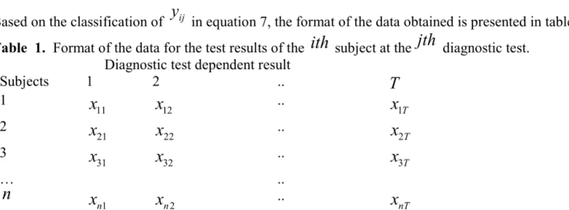
ij _{is the continuous diagnostic test result drawn from population Y.}

Based on the classification of

y

ij in equation 7, the format of the data obtained is presented in table 1.

Table 1. Format of the data for the test results of the

ith

subject at the

jth

diagnostic test. Diagnostic test dependent result

Subjects 1 2 ..

T

1 11

x

x

₁₂ ..

x

1T 2 21

x

x

₂₂ ..

x

_2T 3 31

x

x

₃₂ ..

x

_3T … ..

n

1 n

x

x

_n2 ..

x

_nT

This pattern of coding is appropriate if interest is to compare the AUCs obtained from diagnostic tests processes carried out on the same set of subjects. The coding is such that if a subject’s test result is

x

ij



c

, that subject is considered diseased or response positive(coded 1) while a subject whose test result is

x

ij



c

_{is declared} non-diseased or response negative to the disease (coded 0).

To develop the test statistic for testing the equality of two or more AUCs across different diagnostic tests, Let



1



8

j

p

y

i j







1

9

n j i j i

A n d

f

y







Where

f

j indicated the number of subjects that are diseased or responding positive in the jth diagnostic test while the corresponding subjects who are not diseased or those responding negative is

n



f

j

.

Let 1. 1

10

T j j

n

f

f









1.

n

be the total number of subjects who are diseased for all the diagnostic tests T and let

2. 1

(

1)

11

T j j

n

n

f

n T

f











 

2.

n

be the total number of subjects who are non-diseased or responding negative for all the diagnostic tests. Hence

(

)

;

(

)

(1

)

12

( )

;

( )

(1

)

13

ij j ij j j j j j j j

E y

Var y

and

E f

n

Var f

n

























Where



j is the population proportion of subjects that are diseased or those responding positive for the

jth

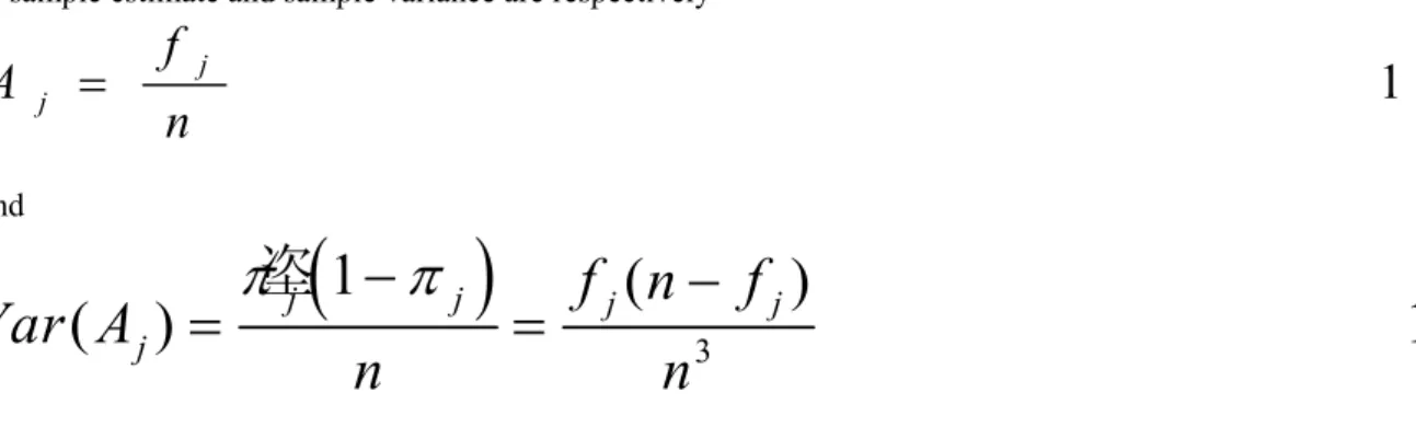
diagnostic test.

Its sample estimate and sample variance are respectively

1 4

j j

f

A

n



And





3

垐

1

(

)

(

_j

)

j j

f n

j

f

j

15

Var A

n

n













Where

A

j_{is actually the area under a portion of the AUC curve of jth diagnostic test. If the proportions of positive} response or diseased subjects are equal for all entire the diagnostic test T, then the common proportion can be estimated as

1 6

f

A

n T



These results are presented in a 2 × Tcontingency table 2.

Table 2. 2 × T Contingency table for the Analysis of diagnostic Test Dependent Measurements. Diagnostic Test Measurements

Observations 1 ….. ……

T

Total

Number of diseased subjects (

f

j₎

f

1 ….. ….

f

T

f

Number of non-diseased subjects (

n



f

j)

n



f

1 ….. …

n



f

T

nT



f

Total

n

….. …

n

nT

Proportion(

A

j₎

A

1 ….. ….

A

T

A

f

nT



Based on table 2, the observed numbers of diseased and non-diseased subjects for the

jth

diagnostic test are respectively

1 j j 2 j j

1 7

o



f

a n d o



n



f

The corresponding expected numbers of diseased and non-diseased subjects are respectively

1

2

(

)

18

j

j

nf

n nT

f

e

and e

nT

nT







The null hypothesis that the AUC of two or more diagnostic tests are equal is stated as

0

:

1 2

...

T 1

:

1 2

...

T

19

H AUC



AUC

 

AUC versus H AUC



AUC

 

AUC

Since AUC summarizes the accuracy or discriminating power of a diagnostic test, then we shall subsequently be viewing the test of hypothesis for AUC in terms of the proportion of positive response rate,



j _{of subjects to tests} because the ability of a test to discriminate among alternative health status (positive and negative response) gives a summary of the diagnostic accuracy of a test. In other words, the probability of positive response of a test if obtained indicates a summary of the accuracy or discriminating power of a diagnostic test given that the proportion of negative response is just a relationship.





2 2 2 1 1

2 0

T i j i j i j i j

o

e

e



 





 

Whose distribution is approximately of the chi-square type having T–1 degrees of freedom and it can be used to test the null hypothesis of equality of AUCs across diagnostic tests.

Writing equation 20 in terms of Equations 14 and 16, we have 2 2 2 1 1

(

)

(

)

(

)

21

(

)

j T T j j j

f

nf

n nT

f

nT

n

f

nf

nT

n nT

f

nT

nT



 











































This simplifies to 2 2 2 1

(

)

2 2

(

1)

T j j

f

f

n T

f n T

T













Equation 22 has also a distribution of the chi-square type with T–1 degrees of freedom.

Rewriting equation 20 in terms of the proportions stated in equations 14 and 16, we have an equivalent expression given as





2 2 1

,

3 0;

1

2 3

T j j

A

A

n

iff nT

q

A

A q













 

At a given level of significance (α), the null hypothesis H0 is rejected if

2

2

1



;

T

1

2 4











Otherwise it is accepted.

SUBSEQUENT ANALYSIS IF NULL HYPOTHESIS IS REJECTED

When the null hypothesis of equations 19 is rejected, it means that differences exist in the AUC across diagnostic tests or the proportion of positive response across diagnostic tests. Therefore, it is of interest to determine which of the AUC or equivalently the proportion of positive response among the diagnostic tests that has contributed to the rejection of H0.In particular, interest may be to determine if the accuracy of diagnostic test result is improving

successively over testing trials or procedures. Let



j _{be the proportion of subjects that are diseased or those} responding positive for the

jth

diagnostic test.

Now let



j

and



k be the population proportions of subjects that are diseased or those responding positive at the

jth and kth

diagnostic tests respectively for

j k

,



1,.., ;

T j



k

.

Its corresponding sample estimates arerespectively,

14.

j

k

j

k

f

f

A

and A

as in equ

n

n





Where

A and A

j k are the areas under a portion of the AUC of

jth and kth

diagnostic tests respectively. Interest here may be in testing the null hypothesis that the proportion of diseased subjects in jth diagnostic test is

at most equal to the proportion of diseased subjects in kth diagnostic test. The null hypotheses may be expressed as

0

:

j k 1

:

j k

;

2 5

H







v e r s u s H







j



k

To test the null hypothesis of equation 25, where the sample estimates of

 

j



k are

A

j



A

k

.

Let









0

2 6

j

k

e

j

k

A

A

z

s

A

A











Where





( )

( ) 2

( ,

);

tan

e j k j k j k

s A



A



Var A



Var A



Cov A A se s



dard deviation

Where

 

 

2 1 1 2

(

,

)

,

1 4

,

1 3

j k j k j k j k j k n n ij sk i s j k

C o v A

A

E

A A

E

A

E A

E

f f

E

f

E

f

see eq u a tio n

n

n

E

y y

see eq u a tio n

n

 

 



















































 



Now

y y

ij

.

skassumes the value 1 provided

y and y

ij skboth assume the value 1 with probability

 

j k

.

Therefore,





2

1

1

2

2

n

n

ij

sk

j

k

i

s

j

k

E y y

n

n

n

 

 



















Hence,

(

j

,

k

)

j

k

j

k

0

Cov A A



   





Therefore,

(

j

k

)

(

j

)

(

k

)

27

Var A



A



Var A



Var A

0

0

(

)

(

)

(

)

( )

( )

j

k

j

k

e

j

k

j

k

A

A

A

A

z

s A

A

Var A

Var A





















which is the unit normal distribution. Hence,





2

0

2

2

(

)

28

( )

( )

j

k

j

k

A

A

z

Var A

Var A





 







has approximately a distribution of the chi-square type with 1 degree of freedom where

A

jis already given in equation 14

And





2

(

j

)

f n

j

f

j

,

15

Var A

see equation

n





Under the null hypothesis of equation 19 and overall estimate of



j_{such as}

A is A

j _{given in equation 16, the} estimate of

Var A

(

j

)

is





3

2

(1

)

(

j

)

A

A

f

n T

f

2 9

V a r A

n

n T









The corresponding test statistic is given as:

2

2

0

0

2

2

30

(

)

(

)

2

( )

j

k

j

k

j

k

f

f

f

f

n

n

n

n

z

Var A

Var A

Var A







































































Where under the null hypothesis





3

2

(

j

)

(

k

)

( )

f nT

f

,

29

Var A

Var A

Var A

see equation

n T













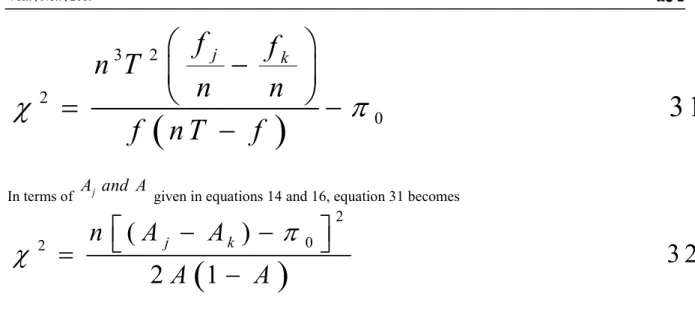
3

2

2

0

3 1

j

k

f

f

n T

n

n

f

n T

f

























In terms of

A and A

j _{given in equations 14 and 16, equation 31 becomes}





2 0 2

(

)

3 2

2

1

j k

n

A

A

A

A





















which has approximately a chi-square distribution with 1 degree of freedom.

The test statistic of equation 32 can be used to test the null hypothesis of equation 25 that the proportion of diseased subjects in the jth diagnostic test is at most equal to the proportion of diseased subjects in the kth diagnostic test. Using this test statistic, it is suggested that all comparison should be made with a well chosen critical value of the chi-squared distribution with T-1 degrees of freedom at a specified



level. This is for the purpose of reducing type 1 error and minimizing errors in conclusions.

METHODOGY

APPLICATION TO REAL DATA

The proposed methods can be applied to real data obtained from a retrospective study of pregnant women at risk for gestational diabetes mellitus (GDM) at certain hospitals in Ebonyi State Nigeria.The records of a total of 1113 pregnant women who had earlier tested positive after screening using 1 hour 50g Glucose Challenge Test (GCT) and who were also subjected to diagnosis using 2-hour 75g OGTT as well as 3-hours 100g OGTT according to WHO(1999) and National Diabetic Data Group(NDDG,1979) criteria were taken. This was to compare the efficacy of these two diagnostic procedures, These pregnant women were seen to have positive risk factors and aged between 15-45 years at less than 24 weeks and between 24-28 weeks of gestation.

Women who were known diabetics, or who were suffering from any chronic illness were excluded from the study. After obtaining permission from the hospitals’ Research and Ethics Committee, assess was granted into the record units of the antenatal wards of these hospitals where the medical history of the patients were kept in a proforma containing general information on demographic characteristics such as body mass index, maternal age, previous fetal weight and vital clinical histories such as obstetric history of GDM and family history of diabetes were taken.

The GDM response variables (tests results) for the two tests, namely 75g OGTT and 100g OGTT represents the paired data for the pregnant women. These data type is suitable for comparing the accuracy of two tests in terms of their AUCs. Under this arrangement, the null hypothesis of interest which is testing of equality of the proportion of positive response is equivalent to testing the equality of AUCs for the tests. This comparison will be evaluated using the proposed method.

The research interest is to compare two or more correlated AUCs of diagnostic tests which also are equivalent to comparing the probability of positive response for paired sample design. To do this, the data was coded for this work based on the specification of equation 7 to generate the corresponding data of 1’s and 0’s. In other to calculate the chi-square test statistic of equation 23 for testing the null hypothesis of no difference among the proportion of positive response (see equation 19) in paired sample design, we evaluate the data for the work to have table 3.

Table 3: Computation of total number of diseased, non-diseased and proportion of diseased. Diagnostic test 1 Diagnostic test 2 Total

No of 1’s

(

f

j

)

146 149 295

No of 0’s

(

n



f

j

)

967 964 1931

Total n 1113 1113 2226

Proportion of 1’s

(

p

j

)

0.1311 0.1339 0.265

sample tests, it was substituted the proportion of 1’s or diseased pregnant women of the data given in equation 23, to calculate the chi-square test statistic as





2 2 2

1113 ( 0.1339)

( 0.1311)

1113 (0.01793) (0.01719)

1113[0.03512]

39.08856

200.96

(0.265)(0.735)

0.194775

0.194775

0.194775











 















At 5% level of significance, where c=2, the chi-square is

2

0.95,1

3.841.





This means that the proportion of positive response for the two diagnostic tests differ significantly. In other words, the two AUC for the tests are different. From Table 3, the proportion of pregnant women who have GDM increased after the second diagnostic test.

Furthermore, our interest may be to determine which of the test is superior or other wise. This is also the same as carrying out further analysis to determine which of the test that may have contributed to our rejecting the null hypothesis of equality of AUCs in equation 19. This means that we need to test the null hypothesis of equation 25. From Table 3, put

p

2



0.1339

and p

1



0.1311,

_{in equation 32 to have}





2 2

1113 0.1311 0.1339

1113 0.00000784

0.0224.

2(0.265)(0.735)

0.38955













If 2

0.0224





is compared with its critical value at

c

   

1

2 1 1

and





0.05

, we accept the null hypothesis of equation 25 and conclude that there exist no significant different between the two diagnostic tests. This simply means that

AUC

2



AUC

1_{.This means that that the second diagnostic test (100g OGTT), that is}

2

AUC

is preferred to first diagnostic test (75g OGTT), that is

AUC

1_{because the second test was able to discover}

few more pregnant women who actually have plasma glucose level of at least 7.8mmol/l(GDM positive patients).

COMPARISON OF THE PROPOSED METHOD WITH DELONG ET AL (1988) METHOD

Using the same coded data meant for comparing AUC, the estimates of AUCs was obtained for the diagnostic tests as 0.687, and 0.752 respectively for the first and second diagnostic test respectively. To test the null hypothesis of equation 19 for the homogeneity of AUCs, the non-parametric test by DeLong et al.(1988) and the proposed chi-square test yielded significant results with their p-values as 0.0068 and 0.0027 respectively.

VALIDATION OF THE PROPOSED METHOD USING COCHRAN Q TEST

To make the proposed method valid in terms of efficiency, we illustrate using Cochran Q test for dichotomous data since the same null hypothesis of equality of AUCs (proportion of diseased pregnant women) across diagnostic tests can suitably be tested. Using the paired coded data which is also applicable, we let

B

i _{be the sum} of the number of 1’s in row i, the pregnant women, where i=1,2,….,1113 and

Z

j k, be the sum of the number of 1’s in column j and k, where j is test 1 and k is test 2. Then the statistic for Cochran’s Q test is given by









2 2 2 2 2 1 1 2 2 2 2 2 1 1

(146)

(149)

(146 149) 2

(

1)

(2 1)

43517 43513

4

295

(2)

(1)

(2)

.... (1)

2

T T j j j j n T i i j

Z

Z

T

Q

T

B

B

T

   















































 

















 

















Which has T-1=2-1=1 degrees of freedom. Since

Q



4

is greater than

2 0.95;1,

3.841





, we reject the null hypothesis of equation 19 which stated the equality of diagnostic tests in terms of their AUCs and conclude that the proportion of pregnant women responding positive (GDM positive patients) and indeed the AUCs differs significantly across tests. This conclusion is the same as that obtained when the proposed method is applied to the same data set. The advantage that the proposed method has over Cochran Q test is that it is capable of finding the reason for rejecting the null hypothesis in the first instance. This implies that subsequent analysis when the null hypothesis is rejected applies to the proposed chi-square method but does not apply to the Cochran method.

DISCUSSION

Many authors have carried out studies for comparing two AUCs(Obuchowski,2005; MacMillan et al,2004; Mackassy and Provost,2004 ) but up till date only two studies have been able to compare more than two AUCs of

several diagnostic tests at once (Delong et al, 1988; Senaratna et al,2015). Some authors developed a bivariate test for comparing two AUCs at a time and included the Bonferroni adjustment for multiple comparison of pairs of AUCs (Senaratna et al, 2015).

DeLong et al (1988) proposed a nonparametric approach to compare the correlated AUCs using the theory of the U-statistics. The disadvantage of this method is that it has computational burden although that can be alleviated by the development of faster computers. Computational burden can still be substantial in binormal ROC curve as a method of calculating AUC because a number of iterative procedures that are involved in obtaining estimators, for instance MLE of AUC (Dorfmann & Alf 1969; Metz, Herman & Shen 1998).

The chi-square test employs a continuous distribution to approximate a discrete probability distribution. Apart from being simple to calculate, easy to understand and readily applicable, the chi-square test statistic provides the quality evidence of inferiority or superiority of one diagnostic process over the other. It does this by providing the opportunity for subsequent analysis to determine the inferiority or other wise of a test when the null hypothesis of interest is rejected. For instance, if the null hypothesis of equality of AUCs is rejected, there is need for further analysis to ascertain which of the AUC or diagnostic test that has contributed to the rejection of the null hypothesis. This is not possible when the Delong et al (1988) method is used for comparing between two AUCs. In using any existing methods, the idea of assessing inferiority or superiority of a diagnostic procedure are not immediately obtainable because sensitivity and specificity simultaneously measures the accuracy of diagnostic procedures (Swets et al, 1982) which always requires the knowledge of true disease status of subjects (Pepe,2003). The proposed method does not require the knowledge of the true disease status or the gold standard may not be known. This is similar to the result obtained using McNemar test for comparing the accuracy of two diagnostic tests for matched sample data (Sumi et al, 2010). This attribute makes the proposed method to have robust feature since it is invariably applicable in all instances in addition to situations where it does require having the knowledge of true status (gold standard).This is not the same with other traditional methods of comparing the accuracy of diagnostic test results such as Bandos et al (2005) and Delong et al(1988)which must require the knowledge of true status (gold standard) in the estimation and comparison using the AUC. Using the proposed chi-square test is simpler and easy to compute than McNemar test proposed by Sumi et al(2010) which can be taken to be a better alternative to the test by DeLong et al.(1988) and test by Bandos et al.(2005) which are very cumbersome to compute.It is known that in the study of the statistical methods for diagnosis, one of the most interesting topics is the comparison of the accuracy of two binary diagnostic tests in relation to the same gold standard (José Antonio et al,2011).For instance, a global hypothesis test was studied to simultaneously compare the positive and negative predictive values of multiple binary diagnostic tests when the binary tests and the gold standard are applied to all of the subjects in a random sample(José Antonio et al,2011).The proposed chi-square method used in comparing the accuracy of two or more diagnostic tests in terms of their AUCs does not make any reference to the gold standard in its comparison. This is indeed an innovation in statistical methods for diagnosis. The AUC were calculated from the parameters a and b obtained using the method of maximum likelihood (Dorfman and Alf, 1969) while the variance of the AUC were calculated using the delta method (Casella and Berger, 2002).These are rather tedious methods, which is why the proposed chi-square method made the calculation of AUC and its variance simpler and easy to understand.

CONCLUSION

This paper concludes as follows

1. That the proposed chi-square test method has higher statistical power when compared with the conventional nonparametric test method (DeLong et al method) and so has the capacity to discriminate between diseased and non-diseased subjects. In other words, the strength of our method is that it has easy implementation to discriminate diagnostic test procedures even by non- statisticians.

2. The proposed chi-square test method is simpler to understand, easy to compute or communicate to the potential users of the procedure to operate than the conventional nonparametric test method.

3. The proposed chi-square test method provides an opportunity for further analysis in a situation where the null hypothesis of interest is rejected. The purpose of this is to determine the possible reason for the rejection of the null hypothesis. This is an advantage over similar methods such as the Cochran Q test method.

4. Knowledge of true status of subjects or any other gold standard is not required to employ by the proposed method in analysis.

5. The proposed method offers reliable statistical inferences even in small sample problems and circumvent the difficulties of deriving the statistical moments of complex summary statistics.

6. The proposed method has the capacity of comparing even more than two AUCs unlike what obtains in other existing methods especially Cochran Q test and Delong method.

7. The proposed method avoids the lengthy and more difficult procedures of estimating the variances of two AUCs as a way of determining if two AUCs differ significantly, rather it developed a simple test statistic for

8. The chi-square test statistic is therefore recommended for comparing the equality of two or more correlated AUCs in paired sample design.

Acknowledgment

I wish to appreciate Dr Happiness Ilouno for her useful contributions and suggestions in ensuring the success of this work.

References

Bandos, A.I., Rockette, H.E., Gur, D. (2005). A permutation test sensitive to differences in areas for comparing ROC curves from a paired design. Statistics in Medicine 24(18), 2873-2893.

Casella, G & Berger, R. L. “Statistical Inference.” Duxbury Press. Second Edition, 2002.

DeLong, E.R., DeLong, D.M., Clarke-Pearson, D.L. (1988). Comparing the area under two or more correlated receiver operating characteristic curves: a nonparametric approach. Biometrics 44(3), 837-845.

Dorfman DD, Alf E. Maximum likelihood estimation of parameters of signal detection theory and determination of Confidence intervals-rating method data. Journal of Mathematical Psychology 1969 ; 6(3): 487-496. Egan, JP. (1975). Signal detection theory and ROC Analysis. New York: Academic Press.

Green, DM. and Swets, JA. (1966). Signal detection theory and psychophysics. John Wiley & Sons, Inc. New York.

Greiner, M., Pfeiffer, D., and Smith, RD. (2000). Principals and practical application of the Receiver Operating Characteristic analysis for diagnostic tests. Preventive Veterinary Medicine, 45:23–41.

J. A. Hanley and B. J. McNeil, “The meaning and use of the area under a receiver operating characteristic (ROC) curve,” Radiology, vol. 143, no. 1, pp. 29–36, 1982.

Hanley JA, McNeil BJ. A method of comparing the Areas under Receiver Operating Characteristic Curves Derived from the same cases. Radiology 1983 ; 148(3): 839-843.

Hanley JA, Hajian-Tilaki KO. Sampling variability of nonparametric estimates of the area under receiver operating characteristic curves: An update. Academ Radiol 1997; 4: 49-58.

Honghu-Liu, Li G, William G. Cumberland and Tongtong Wu .Testing Statistical Significance of the Area under a Receiving Operating Characteristics Curve for Repeated Measures Design with Bootstrapping Journal of Data Science 3(2005), 257-278

Karimollah Hajian-Tilaki .Receiver Operating Characteristic (ROC) Curve Analysis for Medical Diagnostic Test Evaluation.Caspian J Intern Med 2013; 4(2): 627-635

Krzanowski WJ, Hand DJ. ROC curves for continuous data. CRC/Chapman and Hall; 2009.

Kummar R, Indrayan A. Receiver operating characteristic (ROC) curve for medical researchers. Indian Pediatr 2011;

Leisenring, W., Alonzo, T. and Pepe, M.S. 2000. Comparisons of predictive values of binary medical diagnostic tests for paired designs. Biometrics 56, 345-351.

Mackassy SA, Provost F. Confidence Bands for ROC curves. CeDER working paper 02-04, Stern School of Business, New York University, Ny, NY 10012; 2004.

MacMillan NA, Rotello CM, Miller JO. The sampling distributions of Gaussian ROC statistics. Perception and Psychophysics. 2004 ; 66(3) : 406-421.

McClish, DK. (1989). Analyzing a portion of the ROC curve. Medical Decision Making, 9:190–195.

Metz CE, Wang PL, Kronman HB. A new approach for testing the significance of differences between ROC curves from correlated data. In: Deconick F, editor. Information processing in medical imaging. The Hague: Nijhoff; 1984. p.432–45.

Metz, CE., Herman, BA., and Shen, JH. (1998). Maximum likelihood estimation of Receiver Operating Characteristic (ROC) curves from continuously-distributed data. Statistics in Medicine, 17:1033–1053. Moskowitz, C.S. and Pepe, M.S. 2006. Comparing the predictive values of diagnostic tests: sample size and

analysis for paired study designs. Clinical Trials 3, 272-279.

Jayawant N. Mandrekar. Receiver Operating Characteristic Curve in Diagnostic Test Assessment. Biostatistics For Clinicians. J Thorac Oncol. 2010;5: 1315–1316.

Nahid Sultana Sumi, M. Ataharul Islam, and MD. Akhtar Hossain. Evaluation and Computation of Diagnostic tests: A simple Alternative. 2010 mathematics subject classification. 62p10; 92-08; 62-07.

National Diabetes Data Group. Classification and diagnosis of diabetes mellitus and other categories of glucose intolerance. Diabetes 1979; 28: 1039–1057

Obuchowski NA. Fundament of Clinical Research for Radiologists. American Journal of Roentgenology. 2005 ; 184 (2) : 364-372.

Park SH, Goo JM, Jo C. Receiver Operating Characteristic (ROC) curve: Practical review for radiologists. Korean Journal of Radiology. 2004 ; 5(1) : 11-18

University Press.

Pepe, MS. (2004). The statistical evaluation of medical tests for classification and prediction. 1st _{ed. Oxford}

University Press, USA.

Roldán Nofuentes, José Antonio;Luna del Castillo, Juan de Dios; Montero Alonso, Miguel Ángel. Comparison of the predictive values of multiple binary diagnostic tests. Int. Statistical Inst.: Proc. 58th World Statistical Congress, 2011, Dublin (Session CPS039).

D. M. Senaratna, M.R. Sooriyarachchim, and N. Meyen, “Bivariate Test for Testing the EQUALITY of the Average Areas under Correlated Receiver Operating Characteristic Curves (Test for Comparing of AUC’s of Correlated ROC Curves).” American Journal of Applied Mathematics and Statistics, vol. 3, no. 5 (2015): 190-198. doi: 10.12691/ajams-3-5-3.

Swets, J. A. and R. M. Picket, 1982. Evaluation of diagnostic systems: methods from signal detection theory. Academic Press, New York.

Wang, W., Davis, C.S. and Soong, S.J. 2006. Comparison of predictive values of two diagnostic tests from the same sample of subjects using weighted least squares. Statistics in Medicine 25, 2215-2229.

WHO. Definition, Diagnosis and Classification of Diabetes Mellitus and its Complications. Report of a WHO consultation. Part 1: Diagnosis and Classification of Diabetes Mellitus. Geneva: Department of Non-communicable Disease Surveillance, World Health Organization, 1999.