A New Genetic Algorithm for Multi-Label
Correlation-Based Feature Selection
Suwimol Jungjit and Alex A. Freitas School of Computing, University of Kent
Canterbury, UK, CT2 7NF
Abstract. This paper proposes a new Genetic Algorithm for Multi-Label Correlation-Based Feature Selection (GA-ML-CFS). This GA performs a global search in the space of candidate feature subsets, in order to select a high-quality feature subset that is used by a multi-label classification algorithm – in this work, the Multi-Label k-NN algorithm. We compare the results of GA-ML-CFS with the results of the previously proposed Hill-Climbing for Multi-Label Correlation-Based Feature Selection (HC-ML-CFS), across 10 multi-label datasets.
1.
Introduction
A classification algorithm learns, from a training set, a model representing predictive relationships between an instance’s features and its class label(s). The model is then used to predict the class label of previously unseen instances in the test set. In conventional single-label classification, each instance in the data set is associated with just one class label. By contrast, we address a more difficult multi-label classification problem, where each instance can be associated with multiple class labels.
Classification datasets often have a large number of features, so feature selection is often performed in a data pre-processing step, in order to improve predictive performance and eliminate irrelevant and/or redundant features [1].
In this paper we propose a new Genetic Algorithm for Multi-Label Correlation-Based Feature Selection (GA-ML-CFS), and compare its performance against the Hill-Climbing for Multi-Label Correlation-Based Feature Selection (HC-ML-CFS) method proposed in [2], across 10 multi-label classification datasets.
This paper is organized as follows. Section II reviews background on feature selection. Section III describes the proposed GA-ML-CFS method. Section IV reports the computational results. Section VI concludes the paper and mentions future work.
2.
Background on Feature Selection
There are two broad approaches for feature selection in a data preprocessing step: the wrapper and the filter approaches, which are characterized by whether or not (respectively) the feature selection method uses the classification algorithm to measure the quality of candidate feature subsets. Here we use the filter approach, which is much faster and more scalable than the wrapper approach.
There are relatively few published studies on filter feature selection methods for multi-label classification. Many methods first transform the multi-label problem into a single-label one and then use a single-label feature selection method [3,4,5,6,7]. Other works propose feature selection methods that directly cope with multi-label data [8,9,10]. Unlike these works, the new feature selection method proposed here is based on the Correlation-based Feature Selection (CFS) method [11], which has been
recently extended for Multi-label CFS (ML-CFS) in [2,12,13]. ML-CFS searches for features highly correlated with class labels (i.e. relevant features) and features with low correlations among themselves (to avoid the selection of redundant features). ML-CFS uses equation (1) to evaluate the quality of a candidate feature subset F – where L is the set of class labels, k is the number of features in F, r is Pearson’s linear correlation coefficient, 𝑟!" is the average correlation between each feature in F and each class label in L, and 𝑟!! is the average correlation over all pairs of features in F. When computing the terms 𝑟!" and 𝑟!!, we use the absolute value of the correlation coefficient, which improved the predictive performance of ML-CFS in [2].
𝑀𝑒𝑟𝑖𝑡(𝐹)= 𝑘𝑟!"
𝑘+𝑘(𝑘−1)𝑟!!
3.
A New Genetic Algorithm for Multi-Label Feature Selection
We propose a Genetic Algorithm (GA) for Multi-Label Correlation-Based Feature Selection (GA-ML-CFS). GAs are stochastic global search methods inspired by the process of natural selection [14]. There are many GAs proposed as a feature selection method for single-label classification [15,16,17] but developing a GA for multi-label classification seems an unexplored research topic so far.In the proposed GA-ML-CFS each individual (candidate feature subset) is represented by a string of n bits, where n is the number of features. The i-th bit – i = 1,..,n – takes the value 1 or 0 to indicate whether or not a feature is selected, respectively. Each individual is evaluated by a fitness function, given by equation (1). At each generation (iteration), individuals are selected by a combination of an elitism operator and the tournament selection operator, which selects individuals with a probability proportional to their fitness (quality) values. The selected individuals then undergo uniform crossover and bit-flip mutation. The selection, crossover and mutation operators are conventional GA operators [14]; the main novelty of the proposed GA is the multi-label fitness function.
The parameter settings of GA-ML-CFS in our experiments were: population size = 200, number of generations = 100, elitist set size = 4, tournament size = 2, gene crossover probability = 0.5, gene mutation probability = 0.01 – see also Section 4.
4.
Computational Results
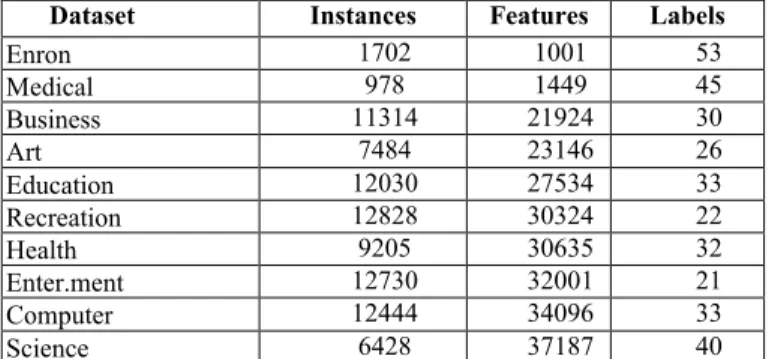
In our experiments, we used 10 multi-label classification datasets (shown in Table I), which were obtained from the multi-label dataset repository website (http://mulan.sourceforge.net/datasets.html) [18]. We used the pre-defined training and test set for each dataset in the above website. In all experiments we use, as a multi-label classification algorithm, the well-known Multi-Label k-Nearest Neighbor (ML-kNN) algorithm [19]. Before running GA-ML-CFS on these 10 datasets, we performed some preliminary experiments to optimize its parameters, using four datasets (CAL500, Scene, Emotions, Yeast, also from the above repository) that are different from the datasets in Table I. This makes it fair to compare the results of GA-ML-CFS with the results of the hill-climbing-based HC-GA-ML-CFS (which has no parameter to be optimized), and evaluates the robustness of the GA’s parameters.
Since all datasets have a very large number of features, we use a univariate filter approach to select the N features with highest average correlation with class labels, before running the GA. The motivation for this initial filtering approach – which is common in GAs for feature selection [15,16,17] – is to reduce the number of features given as input to the GA when the number of features is very large, to reduce the processing time and improve the scalability of GA-ML-CFS. We did experiments with four different numbers of features selected by the univariate filter method (which are also the GA’s individuals’ length): N = 100, 200, 300, 400. Tables 2–5 (each for a different individual length) show the predictive accuracy of ML-kNN when using features selected by the proposed GA-ML-CFS and by the HC-ML-CFS described in [2]. Due to the complexity of evaluating multi-label classification algorithms, Tables 2–5 report results for five measures of multi-label predictive accuracy [20,21]: Average Precision (Avg.Prec.) is to be maximized; while the others – Coverage, Hamming Loss (Ham. Loss), One error and Ranking Loss – are to be minimized.
Dataset Instances Features Labels
Enron 1702 1001 53 Medical 978 1449 45 Business 11314 21924 30 Art 7484 23146 26 Education 12030 27534 33 Recreation 12828 30324 22 Health 9205 30635 32 Enter.ment 12730 32001 21 Computer 12444 34096 33 Science 6428 37187 40
Table 1: Dataset characteristics
Dataset Avg. Prec. Coverage Ham. Loss One Error Rank Loss Avg.Rank GA HC GA HC GA HC GA HC GA HC GA HC Enron 0.58(1) 0.57(2) 13.59(2) 13.55(1) 0.06(2) 0.06(1) 0.4(2) 0.39(1) 0.1(1) 0.11(2) 1.6 1.4 Medical 0.77(1) 0.77(2) 3.32(2) 3.20(1) 0.02(1) 0.02(2) 0.3(1) 0.3(2) 0.05(2) 0.05(1) 1.4 1.6 Business 0.87(1) 0.87(2) 2.39(1) 2.42(2) 0.03(1) 0.03(2) 0.13(1) 0.14(2) 0.04(1) 0.04(2) 1 2 Art 0.53(1) 0.52(2) 5.3(1) 5.31(2) 0.06(1) 0.06(2) 0.58(1) 0.61(2) 0.15(2) 0.13(1) 1.2 1.8 Educat. 0.54(2) 0.54(1) 3.91(2) 3.87(1) 0.04(2) 0.04(1) 0.6(1) 0.6(2) 0.09(2) 0.09(1) 1.8 1.2 Recreat. 0.53(2) 0.54(1) 4.33(2) 4.33(1) 0.06(2) 0.06(1) 0.6(2) 0.6(1) 0.16(1) 0.16(2) 1.8 1.2 Health 0.63(1) 0.63(2) 3.8(1) 3.80(2) 0.05(1.5) 0.05(1.5) 0.48(2) 0.48(1) 0.07(1) 0.07(2) 1.3 1.7 Entertai. 0.57(2) 0.58(1) 3.2(2) 3.19(1) 0.06(2) 0.06(1) 0.58(2) 0.57(1) 0.12(2) 0.12(1) 2 1 Comput. 0.62(2) 0.63(1) 4.38(2) 4.20(1) 0.04(2) 0.04(1) 0.45(1) 0.45(2) 0.09(2) 0.09(1) 1.8 1.2 Science 0.45(1) 0.42(2) 6.86(1) 7.46(2) 0.03(1) 0.04(2) 0.7(1) 0.72(2) 0.14(1) 0.15(2) 1 2 Avg.RK 1.40 1.60 1.60 1.40 1.55 1.45 1.40 1.60 1.50 1.50 1.49 1.51
Table 2: Predictive accuracies for GA-ML-CFS and HC-ML-CFS (individual length = 100) All GA results are an average over 5 runs with a different random seed used to create the initial population in each run. In Tables 2–5, the number in brackets after each measure is the rank (“1” is better than “2”) of each method (GA or HC) for each dataset and for each accuracy measure. The last pair of columns reports the average
rank of each method across all five accuracy measures, for each dataset. The last row reports the average rank for each column (across all 10 datasets).
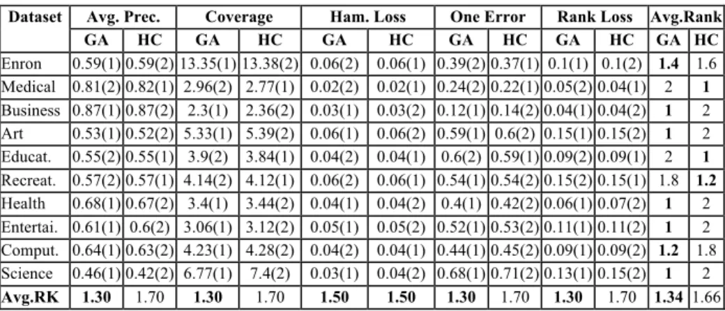
Dataset Avg. Prec. Coverage Ham. Loss One Error Rank Loss Avg.Rank GA HC GA HC GA HC GA HC GA HC GA HC Enron 0.59(1) 0.59(2) 13.35(1) 13.38(2) 0.06(2) 0.06(1) 0.39(2) 0.37(1) 0.1(1) 0.1(2) 1.4 1.6 Medical 0.81(2) 0.82(1) 2.96(2) 2.77(1) 0.02(2) 0.02(1) 0.24(2) 0.22(1) 0.05(2) 0.04(1) 2 1 Business 0.87(1) 0.87(2) 2.3(1) 2.36(2) 0.03(1) 0.03(2) 0.12(1) 0.14(2) 0.04(1) 0.04(2) 1 2 Art 0.53(1) 0.52(2) 5.33(1) 5.39(2) 0.06(1) 0.06(2) 0.59(1) 0.6(2) 0.15(1) 0.15(2) 1 2 Educat. 0.55(2) 0.55(1) 3.9(2) 3.84(1) 0.04(2) 0.04(1) 0.6(2) 0.59(1) 0.09(2) 0.09(1) 2 1 Recreat. 0.57(2) 0.57(1) 4.14(2) 4.12(1) 0.06(2) 0.06(1) 0.54(1) 0.54(2) 0.15(2) 0.15(1) 1.8 1.2 Health 0.68(1) 0.67(2) 3.4(1) 3.44(2) 0.04(1) 0.04(2) 0.4(1) 0.42(2) 0.06(1) 0.07(2) 1 2 Entertai. 0.61(1) 0.6(2) 3.06(1) 3.12(2) 0.05(1) 0.05(2) 0.52(1) 0.53(2) 0.11(1) 0.11(2) 1 2 Comput. 0.64(1) 0.63(2) 4.23(1) 4.28(2) 0.04(2) 0.04(1) 0.44(1) 0.45(2) 0.09(1) 0.09(2) 1.2 1.8 Science 0.46(1) 0.42(2) 6.77(1) 7.4(2) 0.03(1) 0.04(2) 0.68(1) 0.71(2) 0.13(1) 0.15(2) 1 2 Avg.RK 1.30 1.70 1.30 1.70 1.50 1.50 1.30 1.70 1.30 1.70 1.34 1.66
Table 3: Predictive accuracies for GA-ML-CFS and HC-ML-CFS (individual length= 200) Dataset Avg. Prec. Coverage Ham. Loss One Error Rank Loss Avg.Rank
GA HC GA HC GA HC GA HC GA HC GA HC Enron 0.59(1) 0.58(2) 13.25(2) 13.22(1) 0.06(1) 0.06(2) 0.38(2) 0.38(1) 0.1(1) 0.1(2) 1.4 1.6 Medical 0.8(2) 0.81(1) 3.04(2) 2.85(1) 0.02(1) 0.02(2) 0.25(2) 0.24(1) 0.05(2) 0.04(1) 1.8 1.2 Business 0.87(1) 0.87(2) 2.32(1) 2.37(2) 0.03(1) 0.03(2) 0.13(1) 0.14(2) 0.04(2) 0.04(1) 1.2 1.8 Art 0.53(1) 0.51(2) 5.29(1) 5.49(2) 0.06(1) 0.06(2) 0.59(1) 0.62(2) 0.15(1) 0.15(2) 1 2 Educat. 0.55(2) 0.56(1) 3.86(2) 3.77(1) 0.04(2) 0.04(1) 0.6(2) 0.58(1) 0.09(2) 0.09(1) 2 1 Recreat. 0.58(2) 0.59(1) 4.05(2) 3.99(1) 0.05(2) 0.05(1) 0.54(2) 0.53(1) 0.15(2) 0.14(1) 2 1 Health 0.68(2) 0.68(1) 3.41(2) 3.36(1) 0.04(1) 0.04(2) 0.41(1) 0.41(2) 0.06(2) 0.06(1) 1.6 1.4 Entertai. 0.61(2) 0.61(1) 3.05(2) 3.02(1) 0.06(2) 0.05(1) 0.52(1) 0.53(2) 0.11(2) 0.11(1) 1.8 1.2 Comput. 0.64(2) 0.64(1) 4.15(1) 4.19(2) 0.04(1) 0.04(2) 0.44(1) 0.44(2) 0.09(1) 0.09(2) 1.2 1.8 Science 0.46(1) 0.42(2) 6.78(1) 7.41(2) 0.03(1) 0.04(2) 0.67(1) 0.72(2) 0.13(1) 0.15(2) 1 2 Avg.RK 1.60 1.40 1.60 1.40 1.30 1.70 1.40 1.60 1.60 1.40 1.50 1.50
Table 4: Predictive accuracies for GA-ML-CFS and HC-ML-CFS (individual length= 300) In general, GA-ML-CFS obtained better predictive accuracy (lower average rank) than HC-ML-CFS in the experiments with individual lengths of 100 and 200 (Tables 2 and 3). The difference was very small in Table 2, but larger in Table 3, where the GA obtained the better (lower) rank of 1.33, versus 1.66 for the HC. When the individual length is 300 (Table 4), the GA and the HC have the same average rank. When the individual length is 400 (Table 5), the HC obtained the better rank of 1.42, versus 1.58 for the GA. The right part of Table 6 summarizes these results.
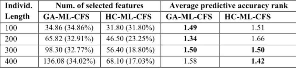
The left part of Table 6 compares the average number and percentage of features selected by each method across all datasets for each individual length. Note that, as the individual length (number of input features) increases, the number of features selected by GA-ML-CFS increases much faster than the number selected by HC-ML-CFS. One possible explanation for this is that the hill-climbing search is more “conservative” than the GA search, as the HC method adds one feature at a time at the current candidate feature subset. Once a good feature subset S1 has been found at
some iteration, the discovery of a much larger feature subset S2 in a later iteration would occur only if each of the extra features had a quality high enough to increase the value of Equation (1). The GA search is less “conservative”, since the crossover operator may add many features at a time to a given individual. Thus, given a feature subset S1, the GA can produce a much larger subset S2 without requiring that each extra feature have a high quality by itself. In theory, this gives the GA the advantage of coping better with feature interactions, but this comes with the disadvantage that the set of extra features added to produce a larger feature subset in a single crossover operation may include some features that are not very relevant for class prediction. This suggests that an interesting future research direction would be to extend the GA’s fitness function with another criterion, introducing some selective pressure to reduce the size of the selected feature subset, although this has to be done carefully in order to avoid reducing the quality of the selected feature subset at the same time.
Dataset Avg. Prec. Coverage Ham. Loss One Error Rank Loss Avg.Rank GA HC GA HC GA HC GA HC GA HC GA HC Enron 0.58(2) 0.59(1) 13.48(2) 13.32(1) 0.06(1) 0.06(2) 0.38(2) 0.38(1) 0.1(2) 0.1(1) 1.8 1.2 Medical 0.8(2) 0.81(1) 3.12(2) 2.88(1) 0.02(1) 0.02(2) 0.25(2) 0.24(1) 0.05(2) 0.05(1) 1.8 1.2 Business 0.87(1) 0.87(2) 2.3(1) 2.39(2) 0.03(1) 0.03(2) 0.13(1) 0.14(2) 0.04(1) 0.04(2) 1 2 Art 0.52(1) 0.52(2) 5.29(1) 5.41(2) 0.06(1) 0.06(2) 0.6(1) 0.61(2) 0.15(1) 0.15(2) 1 2 Educat. 0.55(2) 0.56(1) 3.89(2) 3.8(1) 0.04(2) 0.04(1) 0.6(2) 0.57(1) 0.09(2) 0.09(1) 2 1 Recreat. 0.57(2) 0.59(1) 4.11(2) 4.01(1) 0.06(2) 0.05(1) 0.55(2) 0.53(1) 0.15(2) 0.14(1) 2 1 Health 0.7(2) 0.71(1) 3.29(2) 3.18(1) 0.04(2) 0.04(1) 0.39(2) 0.37(1) 0.06(2) 0.06(1) 2 1 Entertai. 0.62(2) 0.62(1) 2.99(2) 2.97(1) 0.06(2) 0.05(1) 0.52(2) 0.51(1) 0.11(2) 0.11(1) 2 1 Comput. 0.65(1) 0.64(2) 4.13(1) 4.19(2) 0.04(2) 0.04(1) 0.43(1) 0.43(2) 0.09(1) 0.09(2) 1.2 1.8 Science 0.46(1) 0.42(2) 6.82(1) 7.41(2) 0.03(1) 0.04(2) 0.67(1) 0.71(2) 0.13(1) 0.15(2) 1 2 Avg.RK 1.60 1.40 1.60 1.40 1.50 1.50 1.60 1.40 1.60 1.40 1.58 1.42
Table 5: Predictive accuracies for GA-ML-CFS and HC-ML-CFS (individual length= 400) Individ.
Length
Num. of selected features Average predictive accuracy rank
GA-ML-CFS HC-ML-CFS GA-ML-CFS HC-ML-CFS
100 34.86 (34.86%) 31.80 (31.80%) 1.49 1.51 200 65.82 (32.91%) 46.50 (23.25%) 1.34 1.66 300 98.30 (32.77%) 56.40 (18.80%) 1.50 1.50 400 136.08 (34.02%) 68.10 (17.03%) 1.58 1.42
Table 6: Results Summary: average number and percentage of selected features across 10 datasets and average accuracy ranks across 10 datasets and 5 predictive accuracy measures
5.
Conclusion
We proposed the GA-ML-CFS (Genetic Algorithm for Multi-Label Correlation-based Feature Selection) method for selecting features to be used as input by a multi-label classification algorithm. We performed experiments comparing the results of GA-ML-CFS against GA-ML-CFS based on hill-climbing search (HC-GA-ML-CFS), and the GA has obtained somewhat higher predictive accuracies, overall. However, the number of features selected by the GA tends to rapidly increase with an increase in the problem size (number of input features), whilst the HC is less sensitive to this issue.
In future work, we plan to develop a MOGA (Multi-Objective GA) that will use a fitness function with two objectives: the classification accuracy (to be maximized) and the number of selected features (to be minimized). This should help to prevent the GA from selecting too many features.
6.
Acknowledgement:
We thank concurrency researchers at Kent for access to the ‘CoSMoS’ cluster, funded by EPSRC grants EP/E049419/1 and EP/E053505/1.References
[1] H. Lui, H. Motoda, Feature Selection for Knowledge Discovery and Data Mining, Kluwer, 1998. [2] S. Jungjit, A.A. Freitas, M. Michaelis and J. Cinatl, “Two Extensions to Multi-Label
Correlation-Based Feature Selection: a case study in bioinformatics,” in Proc. 2013 IEEE Int. Conf. on Systems, Man and Cybernetics, Manchester, UK, 2013.
[3] G. Doquire and M. Verleysen, “Feature Selection for Multi-label Classification Problems,” in Lecture Notes in Computer Science, vol. 6691, pp. 9-16, Springer, Heidelberg 2011.
[4] G. Doquire and M. Verleysen, “Mutual Information Based Feature Selection for Multi-Label Classification.” Neurocomputing, 122(2013), pp. 148-155, 2013.
[5] W. Chen, J. Yan, B. Zhang, Z. Chen and Q. Yang, “Document transformation for multi-label feature selection in text categorization,” in Proc. IEEE Int. Conf. on Data Mining, pp. 451–456, 2007. [6] N. Spolaor, E.A. Cherman and M.C. Monard, “Using ReliefF for Multi-label feature selection,” in
Proceedings of Conferencia Latinoamericana de Informatica, pp. 960-975, 2011.
[7] N. Spolaor and G.Tsoumakas, “Evaluating Feature Selection Methods for Multi-Label Text Classification”, BioASQ Workshop, Valencia, Spain, September 27, 2013.
[8] G. Lastra, O. Luaces, J. R. Quevedo and A. Bahamonde, “Graphical Feature Selection for Multilabel Classification Tasks.” in Proceedings of the 10th international conference on Advances in Intelligent Data Analysis X. Lecture Notes in Computer Science, vol. 7014, Springer, pp. 246-257, 2011. [9] M. L. Zhang, J. M. Pena, V. Robles, “Feature selection for multi-label naive Bayes classification.”
Information Science, vol. 179(19), pp. 3218-3229, 2009.
[10] N. Spolaor, E.A. Cherman, M.C. Monard and H. D. Lee, “Filter Approach Feature Selection Methods to Support Multi-label Learning Based on ReliefF and Information Gain,” in SBIA 2012, Lecture Notes in Artificial Intelligence, vol.7589, L. N. Barros et al, Eds, Springer, pp.72-81, 2012. [11] M. A. Hall, “Correlation-based Feature Selection for Discrete and Numeric Class machine
Learning,” in Proc. 17th Int. Conf. on Machine Learning (ICML-2000), pp.359-366, 2000. [12] S. Jungjit, A.A. Freitas, M. Michaelis and J. Cinatl, “A Multi-Label Correlation Based Feature
Selection Method for the Classification of Neuroblastoma microarray data”, in Advances in Data Mining: 12th Industrial Conference (ICDM 2012): Workshop Proceedings – Workshop on Data Mining in Life Sciences (DMLS 2012), IBAI Publishing, pp. 149-157, 2012.
[13] S. Jungjit, A.A. Freitas, M. Michaelis and J. Cinatl, “Extending Multi-Label Feature Selection with KEGG Pathway Information for Microarray Data Analysis,” in Proc. 2014 IEEE Int. Conf. on Computational Intelligence in Bioinform. and Computational Biology (CIBCB2014), May 2014. [14] A. E. Eiben and J. E. Smith, “Introduction to Evolutionary Computing”, Springer, 2003.
[15] F. Tan, X. Fu and Y. Zhang, “A genetic algorithm-based method for feature subset selection”, Soft Computing, 12(2), pp. 111-120, 2008.
[16] C. H. Yang, L. Y. Chuang, and C. H. Yang. "IG-GA: a hybrid filter/wrapper method for feature selection of microarray data." Journal of Medical and Biological Engineering 30, no. 1(2010): 23-28. [17] L. Y. Chuang, C. H. Yang, K. C. Wu, and C. H. Yang. "A hybrid feature selection method for DNA
microarray data." Computers in biology and medicine 41, no. 4 (2011): 228-237, 2011.
[18] G. Tsoumakas, E. Spyromitros-Xioufis, J. Vilcek, I. Vlahavas, “Mulan: A Java Library for Multi-Label Learning”, Journal of Machine Learning Research, 12, 2011 pp. 2411-2414.
[19] M. L. Zhang and Z. H. Zhou, “ML-KNN: a lazy learning approach to multi-label learning,” Pattern Recognition, 40(7), pp. 2038-2048, 2007.
[20] E. C. Gonçalves, A. Plastino, and A. A. Freitas. "A Genetic Algorithm for Optimizing the Label Ordering in Multi-label Classifier Chains." In Tools with Artificial Intelligence (ICTAI), 2013 IEEE 25th Int. Conf. on, pp. 469-476, IEEE, 2013.
[21] G. Tsoumakas, I. Katakis, I. Vlahavas, “Mining Multi-label data,” in Data Mining and Knowledge Discovery Handbook, O. Maimon, L. Rokach, Eds. , pp. 667-685 Springer, 2010.