UNIVERSIDAD AUTÓNOMA DE MADRID
ESCUELA POLITÉCNICA SUPERIOR
Double degree in Computer Science and Mathematics
DEGREE WORK
Functional data analysis: interpolation,
registration, and nearest neighbors in scikit-fda
Author: Pablo Marcos Manchón
Advisor: Alberto Suárez González
http://creativecommons.org/licenses/by-nc-sa/3.0/
You are free to share (copy, distribute and transmit) and to modify the work under the following conditions:
• You must attribute the work in the manner specified by the author
or licensor (but not in any way that suggests that they endorse you or your use of the work).
• You may not use this work for commercial purposes.
• If you alter, transform, or build upon this work, you may distribute
the resulting work only under the same or similar license to this one. RIGHTS RESERVED
© June 2019 por UNIVERSIDAD AUTÓNOMA DE MADRID Francisco Tomás y Valiente, nº 1
Madrid, 28049 Spain
Pablo Marcos Manchón
Functional data analysis: interpolation, registration, and nearest neighbors in scikit-fda
Pablo Marcos Manchón
The mathematician’s patterns, like the painter’s or the poet’s must be beautiful; the ideas like the colours or the words, must fit together in a harmonious way. G.H. Hardy, A Mathematician’s Apology
A
gradecimientos
En primer lugar me gustaría dar las gracias a todas las personas junto a las que he trabajado durante este proyecto. A Alberto, por darme la oportunidad de formar parte del equipo y guiarme a lo largo de este trabajo, dándome libertad para enfocarme en aquellas partes que más me motivaban. A Carlos, por su dedicación y sus exhaustivas revisiones, sin las cuales este proyecto no sería lo que es a día de hoy y a Jose Luis, por sus inestimables aportaciones matemáticas. Finalmente a Manso y Amanda, junto a los cuales he tenido el placer de compartir este trabajo a lo largo del año.
Además me gustaría agradecer el apoyo de mi familia y amigos, el cual ha sido fundamental en esta etapa. En especial a mis padres, sin los cuales nada de esto habría sido posible, a Sergio, por haber estado desde el inicio de los tiempos, y a Lucía, por compartir conmigo este camino y sin la cual todo habría sido muy diferente.
R
esumen
El análisis de datos funcionales (FDA) es una rama de la estadística dedicada al estudio de can-tidades aleatorias que dependen de un parámetro continuo, como series temporales o curvas en el espacio. En FDA, los datos pueden ser vistos como funciones aleatorias muestreadas de un proceso estocástico subyacente.
Es este trabajo consideraremos tres tareas diferentes en FDA: el uso de técnicas de interpolación para estimar valores de las funciones en puntos no observados, el registro de este tipo de datos y los problemas de clasificación y regresión cuando las instancias son caracterizadas por atributos funcionales. En particular, en este proyecto se han extendido las funcionalidades del paquete de Python
scikit-fdapara dar soporte a estas tres áreas.
En general, las instancias de datos consideradas en FDA están formadas por una colección de observaciones medidas en valores discretos del parámetro del que dependen (p. ej. tiempo o espacio). Para algunas aplicaciones es conveniente, y en algunos casos necesario, estimar el valor de estas funciones en puntos no observados. Esto puede lograrse mediante el uso de interpolación a partir de las mediciones disponibles.
En algunas aplicaciones, las funciones observadas tiene formas similares, pero presentan una va-riabilidad cuyo origen proviene de distorsiones en la escala del parámetro continuo del que dependen. El registro de los datos consiste en caracterizar esta variabilidad y eliminarla de la muestra.
En este trabajo también se abordan los problemas de clasificación y regresión con datos de na-turaleza funcional. Concretamente, se han diseñado estimadores de vecinos próximos, basados en la noción de cercanía entre muestras.
En particular, en este trabajo se ha extendido el paquetescikit-fdapara incluir métodos de interpo-lación basados en splines. También se ha dotado el paquete con herramientas para el registro de datos usando traslaciones, puntos de referencia o para el registro elástico, el cual hace uso de la métrica de Fisher-Rao para alinear las funciones de una muestra. Además, se han incluido modelos basados en vecinos próximos para realizar regresión, tanto con respuesta escalar como funcional, y clasificación.
P
alabras clave
A
bstract
Functional Data Analysis (FDA) is a branch of Statistics devoted to the study of random quantities that depend on a continuous parameter, such as time series or curves in space. In FDA the data instances can be viewed as random functions sampled from an underlying stochastic process.
In this work we consider three different tasks in FDA: the use of interpolation techniques to estimate the values of the functions at unobserved points, the registration of these type of data, and the solu-tion of classificasolu-tion and regression problems in which the instances are characterized by funcsolu-tional attributes. In particular, in this project thescikit-fdapackage for FDA in Python has been extended with functionality in these areas.
Generally, the data instances considered in FDA consist of a collection of observations at a discrete values of the parameter on which they depend (e.g. time or space). For some applications it is conve-nient, and in some cases necessary, to estimate the value of these functions at unobserved points. This can be achieved through the use of interpolation from the available measurements.
In some applications, the functions observed have similar shapes, but exhibit variability whose ori-gin can be traced to distortions in the scale of the continuous parameter on which the data depend. Registration consists in characterizing this variability and eliminating it from the sample considered.
In this work we also address classification and regression problems with data that are characterized by functions. Specifically, we design nearest neighbors estimators based on the notion of closeness among samples.
Specifically, in this work thescikit-fdapackage has been extended to include interpolation methods based on splines. The package has also been endowed with tools for data registration using either shifts, landmark alignment, or elastic registration, which makes use of the Fisher-Rao metric to align the functions in a sample. In addition, models based on nearest neighbors have been included to carry out regression, with both scalar and functional response, and classification.
K
eywords
T
able of
C
ontents
1 Introduction 1
1.1 Goals and scope . . . 2
1.2 Document Structure . . . 2
2 State of the art: interpolation, registration, and nearest neighbors 3 2.1 Interpolation . . . 4
2.1.1 Linear interpolation . . . 5
2.1.2 Spline interpolation . . . 5
2.1.3 Smoothing spline interpolation . . . 7
2.2 Registration . . . 8
2.2.1 Shift registration . . . 9
2.2.2 Warping functions . . . 10
2.2.3 Landmark registration . . . 11
2.2.4 Pairwise and groupwise alignment . . . 12
2.2.5 Amplitude phase decomposition . . . 14
2.3 Elastic methods in functional data analysis . . . 15
2.3.1 Fisher-Rao metric . . . 15
2.3.2 Amplitude and phase spaces . . . 18
2.3.3 Pairwise alignment . . . 20 2.3.4 Karcher means . . . 21 2.3.5 Elastic registration . . . 22 2.3.6 Restricting elasticity . . . 23 2.4 Nearest neighbors . . . 24 2.4.1 Classification . . . 26 2.4.2 Regression . . . 26
3 Design and development 27 3.1 Analysis . . . 28
3.2 Design . . . 28
3.2.1 Representation module . . . 29
3.2.2 Preprocessing module . . . 30
3.2.3 Machine learning module . . . 30
3.2.4 Miscellaneous module . . . 31
4 Conclusions and future work 35
Bibliography 38
Acronyms 39
Appendices
41
A Algorithms and proofs 43
A.1 Shift registration by the Newton-Raphson algorithm . . . 43
A.2 Proofs of some mathematical results . . . 44
B Example notebooks 47
C Programmer’s guide 73
L
ists
List of equations
2.1 Linear interpolation . . . 5
2.2 Smoothing condition . . . 7
2.3 Shift registrtion. . . 9
2.4 Least square criterion . . . 9
2.5 Warping registration. . . 10
2.6 Warping mapping of landmarks. . . 11
2.7 Creterion for pairwise alignment . . . 12
2.8 Lack of symetry . . . 13
2.9 Mean square error total. . . 14
2.10 Mean square decomposed. . . 14
2.11 Square multiple correlation index. . . 14
2.12 Fisher-Rao metric . . . 16
2.13 Length of path . . . 16
2.14 Length of shortest path. . . 16
2.15 SRSF of composition. . . 17
2.16 Elastic distance . . . 19
2.17 Norm of warping. . . 19
2.18 Phase distance. . . 20
2.19 Relative phase . . . 20
2.20 Pairwise alignment with F-R metric. . . 20
2.21 Inverse consistency. . . 20
2.22 Karcher means. . . 21
2.23 Karcher mean onA . . . 22
2.24 Identity mean . . . 23
2.25 Restricted amplitude distance . . . 23
2.26 Classification prediction . . . 26
2.27 Regression response. . . 26
3.1 Evaluation of functional data . . . 29
A.1 First derivative of REGSSE . . . 43
A.2 Second derivative of REGSSE. . . 43
2.2 Example of linear interpolation . . . 5
2.3 Example of spline interpolation. . . 6
2.4 Interpolation of surface. . . 6
2.5 Example of smoothing . . . 7
2.6 Male growth rate . . . 8
2.7 Amplitude and phase variability . . . 9
2.8 Shift registration of a dataset. . . 10
2.9 Set of warping functions. . . 11
2.10 Shift registration of a dataset. . . 11
2.11 Pairwise alignment . . . 12
2.12 Pinching force effect. . . 13
2.13 Tangent space of tridimensional manifold . . . 15
2.14 Geodesic path inF. . . 17
2.15 Action ofΓ . . . 17
2.16 Rotation in complex plane . . . 18
2.17 Phase and amplitude in the complex plane. . . 18
2.18 Functions in the same orbit . . . 19
2.19 Karcher mean of dataset . . . 21
2.20 Scheme of the elastic registration procedure . . . 22
2.21 Elastic registration of the Berkeley velocity curves. . . 23
2.22 Penalized elastic registration. . . 24
2.23 Neighborhoods using distanceL∞. . . 25
3.1 Scikit-fda logo . . . 27
3.2 Map of scikit-fda . . . 29
3.3 Scikit-fda online documentation . . . 32
3.4 Doctest. . . 33
3.5 Example of git flow branches. . . 34
1
I
ntroduction
Functional data analysis (FDA), is a branch of Statistics that deals with the study of random
varia-bles of functional nature, such as time series or curves in the space. It is a relatively recent field, whose first references began in the 1950s, with various articles related to the study of stochastic processes. However, it was not until 1982 with the publication by J.O. Ramsay ofWhen the data are functions [1] when the termFDA began to be used to denote this field. Since then, and especially in the last two decades, techniques used for this analysis have evolved quickly, as well as their applications in a wide range of fields such as medicine, bioinformatics or engineering.
Due to their continuous structure, the data treated in FDAare viewed as functions. However, fun-ctional data are generally observed and recorded as a discrete set of measures. For this reason, one of the first tasks to be performed inFDAis the representation of these data as continuous functions. One of the main approaches to address this task is the use of interpolation for the construction of continuous functions from these discrete measurements.
Once the data are in functional form, it is possible to perform further analysis, such as studying the variability of a set of samples. Unlike other types of data, due to their functional nature, the variability of a set of functional samples may come from their internal structure, such as the time scale in which a process takes place. For this reason, it is necessary to incorporate a stage in the analysis in which this variability is quantified and separated. This step is called registration.
Throughout this work we will focus primarily on three areas of FDA: the use of interpolation for data representation, the registration, and the use of nearest neighbors estimators on classification and regression problems with functional data.
There are some software solutions in R and Matlab that provide support to this field, such asfda[2] [3]; orfda.usc [4], developed by a team at the University of Santiago de Compostela. Inspired by these solutions, in 2017, thescikit-fda project arose under the namefda [5], as part of a Bachelor’s degree thesis made by Miguel Carbajo at the UAM. The aim of this work was to initiate the creation of a Python package to give support to this field, under the philosophy of an open-source project, along with the creation of a community that contributes to its development and maintenance.
Currently, the project is being driven by the Machine Learning Group at the UAM together with the contributions of several undergraduate thesis, such as this one. The package is already in use by some researchers and was presented in theIII International Workshop on Advances in Functional Data Analysis[6].
1.1.
Goals and scope
The aim of this work is to extend the functionality provided by thescikit-fdasoftware package. The functionalities that will be developed during this work may be divided into three main areas.
Firstly, interpolation techniques will be integrated with the existing structures for the representation of functional data. These original structures do not allow the evaluation of functional data as if they were functions, which will be possible after the incorporation of the contributions of this work.
Secondly, tools will be created to the data registration. For this task the books Functional data
analysis[7] andFunctional and shape data analysis[8] have been taken from reference. As a result of
these contributions, the package will provide anAPIto perform this step of the analysis.
To conclude, classification and regression models based on nearest neighbours will be incorporated. For this purpose, the estimators of thescikit-learn[9]APIwill be used as a reference, incorporating an extension of these estimators for functional data into thescikit-fdapackage.
1.2.
Document Structure
The main part of the present document is divided into three chapters, aside from this introduction part. In the Chapter2, it is exposed the state of the art, which gives an overview of the mathematical framework of the functionalities developed to the package.
Chapter3summarizes the analysis and design of the functionalities added to the package, as well as the methodology and technologies used during the development of the work. To finish the main part, Chapter4presents the conclusions of the work done along with a brief discussion about future work.
Besides, this document appends three annexes. In AnnexA there are more detailed descriptions of the different algorithms used, along with proofs of some mathematical results set out in Section2.3, which have been moved to the annexes for the sake of clarity.
Finally, AnnexBincludes a series of Python notebooks showing examples of the use of the functio-nalities incorporated, which have been thought to show in a pleasant way how to use the package to a new user. The documentation of the software developed has been include in the AnnexC.
2
S
tate of the art
:
interpolation
,
registration
,
and nearest neighbors
In FDA, the analyzed data can take the form of temporal series, curves, surfaces or any process that varies over a continuum. The observations that make up our data come from random variables, whose realizations take values in functional spaces, that is to say, they are realizations of stochastic processes. For this reason, they can be viewed as random functions.
In practice, the information of a functional datum f(t) is observed and recorded as pairs (tj, yj),
whereyj is a snapshot of the functionf attj, i.e.,f(tj). One may wonder what makesFDAdifferent
from multivariate analysis, considering the fact that data is generally recorded and stored in the form of observations at discrete points [8]. In multivariate statistics one works with the vector of values{yj},
applying statistical methods and vector calculus to its study, but without taking into account the high correlation between the valuesyj, and yj+1, due to the continuous structure given by the parameter
on which they vary. However, FDAkeeps the association of valuesyj andtj, taking into account the
functional nature of the data, allowing the study of the data using functional calculus. Since the obser-vations are functions, dependent on one or several continuous parameters, such as the time in which a process takes place, it is not possible to measure and store all the points which they are defined for.
There are two main approaches inFDAto represent the data while preserving its functional struc-ture. The first, calleddiscrete representation, stores in a finite grid the pairs(tj, yj)which representes
the valuesf(tj). Interpolation is used to reconstruct the data as a continuous function from its discrete
values.
The second one is a parametric approach, called basis representation, in which is considered a system of functions{φk(t)}Kk=1, such as a truncated Fourier basis or a set of polynomials. This system
forms a finite subspace of the original functional space, where the observations are projected, obtaining a representation associated to the coefficients of the basisf(t)≈PK
k=1ckφk(t).
Due to this functional structure in the data,FDAneeds to address some issues that do not arise when studying other types of data, such as vectors. For instance, once our data is represented as a set of functions{fi(t)}ni=1, its variability can proceed from two sources, the random curve-to-curve
variation, i.e., the difference between the values of the functions, or from the internal structure of its domain. It is fundamental to study and quantify these two types of variability in the analysis of our data.
This separation is called the registration of the data, and is treated in detail in the Section2.2.
FDA also deals with topics present in classical statistics in cases where the data are functions. Among these problems are the study of regression and classification models. In the Section2.4the use of nearest neighbors estimators applied to functional data is studied.
Although inFDAis also treated the case in which our data are multivariate functions, fromRdtoRm, in general, as a way of simplification, during this chapter we will assume that our data are univariate functions.
In this chapter is made an overview, from a theoretical point of view, of differentFDAtopics covered in this work. However, this chapter also serves to introduce the functionalities included in thescikit-fda
package. The figures shown throughout this section have been made using these functionalities.
2.1.
Interpolation
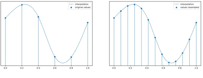
In the discrete representation, frequently, it is necessary to resample or evaluate the data, or its derivatives, at points within the domain range, different that the original pairs{(tj, yj)} at which our
observations have been measured. An example of this it is shown in the Figure2.1. For this purpose interpolation is used. This allows to treat each functional datum as a single entityf(t), which varies continuously throughoutt.
0.0 0.2 0.4 0.6 0.8 1.0
interpolation original values
(a) Original observation
0.0 0.2 0.4 0.6 0.8 1.0
interpolation values resampled
(b) Observation resampled
Figure 2.1:Function resampled using interpolation
Although they are not the only methods used for interpolation, splines and smoothing splines are the most used, for this reason we will focus on them during this work.
2.1. Interpolation
2.1.1.
Linear interpolation
Given two points tk and tk+1 for which the values of our function are known, denoted by yk and yk+1, we can use a line segment to join these values as a first approach. Using this interpolation, we
will obtain a piecewise linear function, whose values in the interval[tk, tk+1]are be given by f(t) =yk+
yk+1−yk tk+1−tk
(t−tk). (2.1)
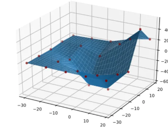
In the case of multivariate functions, multilinear interpolation generalizes this method to higher di-mensions. The same principles are applied, but the piecewise domain is composed by regions calcula-ted using triangulation, and the evaluation is performed using a multilinear form, obtaining in the case of surfaces piecewise functions formed by plane sections. In the Figure 2.2it is plotted the result of interpolating a temporal series and a surface.
0.0 0.2 0.4 0.6 0.8 1.0 0.25 0.50 0.75 1.00 1.25 1.50 1.75 2.00
(a) Linear interpolation
30 20 10 0 10 20 30 20 100 1020 60 40 20 0 20 40 (b) Bilinear interpolation
Figure 2.2:Example of linear interpolation
2.1.2.
Spline interpolation
In spline interpolation [10], the points are linked by a piecewise polynomial. The main advantage of using splines of orderp, i.e., using polynomials of order pin the different intervals, is that we will not only obtain continuous functions, as in the linear case, but we will also obtain functionsCp−1[a, b], i.e.,
that are continuous and havep−1continuous derivatives. This fact is crucial inFDA, because we will need to use derivatives in many parts of the analysis.
To achieve this, we have to match the values of the derivatives of the adjacent splines in the inter-polation knots. If we denote bysk(t) =
Pn
j=0cjktk to the spline defined in the region[tk−1, tk], during
0.0 0.2 0.4 0.6 0.8 1.0 0.00 0.25 0.50 0.75 1.00 1.25 1.50 1.75 2.00 linear cuadratic cubic
(a) Spline interpolation
0.0 0.2 0.4 0.6 0.8 1.0 8 6 4 2 0 2 4 6 8 linear cuadratic cubic (b) First derivatives
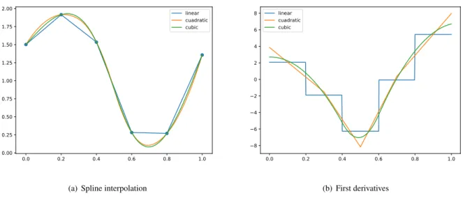
Figure 2.3:Example of spline interpolation
d= 1, . . . , p−1. For this purpose, we will define a linear system of equations which can be solved ite-ratively. Figure2.3(a)shows the result of interpolate a temporal series using splines of different orders, and the first derivatives of these splines, which are splines of orderp−1due to the derivation of the polynomials. 30 20 10 0 10 20 30 20 100 1020 60 40 20 0 20 40 60
(a) Surface interpolated
30 20 10 0 10 20 30 20 100 1020 3 21 0 12 34 (b) Partial derivative∂x
Figure 2.4:Interpolation of surface with bicubic splines
We can extend spline interpolation for multivariate functions, such as surfaces, where bivariate splines will be used. In this case, triangulation is used to calculate the regions in which the polynomials are defined. These polynomials are of the forms(x, y) = P
0≤i+j≤nci,jxiyj. In the Figure 2.4(a)it is
shown the result of the interpolation of a surface using bicubic splines and the partial derivative respect to its first parameter.
2.1. Interpolation
2.1.3.
Smoothing spline interpolation
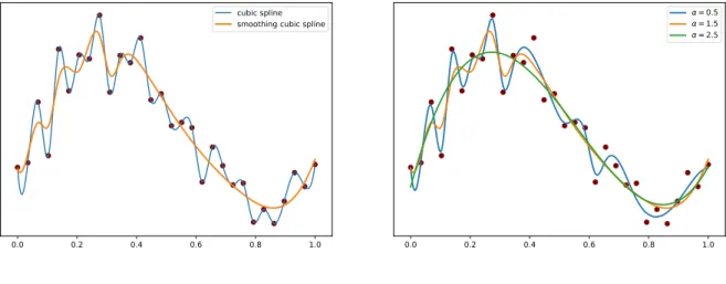
In several contexts, the functional data are contamined with noise. This contamination can be due to errors in the measure procedure or to the intrinsic random behaviour of the process, this will motivate the use of smoothing splines.
0.0 0.2 0.4 0.6 0.8 1.0
cubic spline smoothing cubic spline
(a) Cubic smoothing
0.0 0.2 0.4 0.6 0.8 1.0
= 0.5 = 1.5 = 2.5
(b) Several values of the smoothing factor
Figure 2.5:Smoothing interpolation
This method is a variant of the spline interpolation, wich not uses directly the points {tk}Nk=1 as
knots. Instead, it is used a smaller set of knots{˜tk}M
k=1, generally different from the originals, with their
corresponding valuesy˜k =f(˜tk)calculated using spline interpolation. The function interpolated using
smoothing splines is defined using spline interpolation on the set of knots(˜tk,y˜k). Figure2.5shows the
smoothing interpolation of a noisy observation.
To determine the knots˜tk is used an smoothing parameterα. A weightwk is assigned to each of
the original pointstk, used to calculate the knotst˜k as a weighted average of the original ones. These
weights can be set uniformly. The number of knows will be increased until the smoothing condition is satisfied, defined as N X k=1 wk yk−f˜(tk) 2 ≤α (2.2)
wheref˜(tk)is the value of the smoothing spline attk. In other words, the smoothing parameter sets
the maximum value of the residuals.
After representing the data as continuous functions, we can move on to other parts of the analysis, such as the study of variability due to the continuous structure of the data, called registration of the data. The techniques used during the registration of the data require the use of a discrete representation of the functions and their evaluation in arbitrary points, which is done by interpolation.
2.2.
Registration
In many situations, functional observations have similar shapes, but they are in some way misalig-ned. This variability can interfere with further analysis. Therefore, it is desirable quantify and eliminate or reduced this variation. This process is calledregistration.
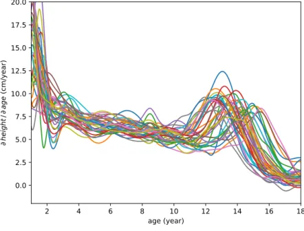
2 4 6 8 10 12 14 16 18 age (year) 0.0 2.5 5.0 7.5 10.0 12.5 15.0 17.5 20.0 he igh t/ ag e ( cm /ye ar )
Figure 2.6:Male growth rate
To illustrate the problem we consider functional data from the Berkeley Growth Study [11]. In this 1954 study, the heights of 54 girls and 39 boys between the ages of 1 and 18 years were recorded. In Figure2.6velocity growth curves of the boys are shown. These curves correspond to the derivatives of the growth curves. In them this type of variability may be appreciated in a more pronounced way. Every curve shows a main stage of growth corresponding with the puberty; however, these stages are not aligned due to hormonal and other physiological factors in the growth. The rigid metric of physical time may not be directly relevant to the internal dynamics of our problem. Thus it may be convenient to make a transformation of the time scale to adapt it to the nature of our data. In the registration of the data, or alignment, this type of variability is analyzed, quantified and separated.
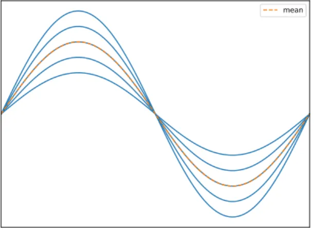
The variability of the data can be analyzed in terms of amplitude and phase variation. Amplitude
variationcorresponds to the random curve-to-curve variation. In the Figure2.7(a)a set of curves whose
variability proceeds exclusively from the amplitude is shown.Phase variationrefers to misalignments of the curves with respect to its domain. In the Figure2.7(b)a set of curves whose variation is completely due to the phase is shown; this source of variability is the one that will be dealt with in the registration process.
2.2. Registration
mean
(a) Dataset with amplitude variability
mean
(b) Dataset with phase variability
Figure 2.7:Amplitude and phase variability
2.2.1.
Shift registration
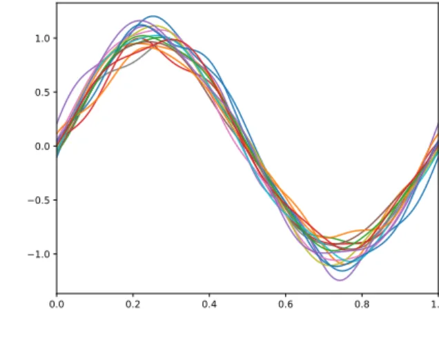
A first approach to solve this problem was presented in Ramsay and Silverman (2005) [7], by con-sidering a simple shift in the domain to make the registration. Although it is a basic approach, it will be useful in many cases. Figure 2.8(a)shows a set of sinusoidal waves whose phases are not aligned, and a shift in the time scale will be adequate to make the alignment.
Let{fi}ni=1 be a set of functional observations, which will be aligned using this transformation. We
are actually interested in finding the values
fi∗(t) =fi(t+δi) i= 1,2, . . . n (2.3)
where the shift parameter δi is chosen in order to align the features of the curves. In the Figure
2.8(b)it is shown the result of apply this type of transformation to the set of sinusoidal waves.
A possible solution for the calculation of shiftsδi, is using a least square criterion, minimizing the
Registered sum of squared errors (REGSSE), defined as
REGSSE= n X i=1 Z T [fi(t+δi)−µˆ(t)]2dt (2.4)
whereµˆ(t)is the mean of the registered functionsfi(t+δi).
The alignment problem will be based on finding the valuesδi that minimize this sum of errors. For
this purpose, we will use the derivatives of the functionsxi, using a variant of the Newton-Rhapson
0.0 0.2 0.4 0.6 0.8 1.0 1.0 0.5 0.0 0.5 1.0
(a) Unregistered curvesx(t)
0.0 0.2 0.4 0.6 0.8 1.0 1.0 0.5 0.0 0.5 1.0 (b) Registered curvesx∗(t)
Figure 2.8:Shift registration of a dataset
2.2.2.
Warping functions
In most cases, it is necessary to consider a more general transformation than a simple translation; generally, this transformation will not be linear. In the case of univariate functional data, i.e., the case that the functions under analysis depend on a single continuous parameter, we will have functions
fi :T ⊂ R→ R, in such a way that we can understand the problem as the search for an appropriate
parameterization of our data, according with the intrinsic structure of the dataset.
We will consider the functionsγi :T → T, referred to as warping functions in the related literature,
that we will use to reparametrize the domain, i.e, to change the internal scale of the data. Using these warping functions we will obtain the curves registered by means of composition of functions, i.e.,
fi∗(t) =fi(γi(t)) =fi◦γi. (2.5)
So that the alignment does not alter the structure of the functional data, these functions γi must
be boundary-preserving dipheomorphisms. A dipheomorphisms is an invertible function that maps one differentiable manifold to another such that both the function and its inverse are smooth. In our case the dipheomorphisms maps the domain of the functionsfi,T, to itself. The boundary-preserving condition
imposes that the border ofT is not altered by the warping functions. In the case where the domain of the functionsT is an interval[a, b], the warpings will be strictly increasing functions that fix the bounds of the domain, i.e.,γi(a) =aandγi(b) =b, as could be seen in the Figure2.9.
Without loss of generality, in the following sections, we will assume that T = [0,1], because the general caseT = [a, b]can be reduced to this with an affine transformation. Also, we will denote the set of such warping functions asΓ.
2.2. Registration 0.0 0.2 0.4 0.6 0.8 1.0 0.0 0.2 0.4 0.6 0.8 1.0 identity id
Figure 2.9:Set of warping functions defined inT = [0,1]
2.2.3.
Landmark registration
A possible solution to register a dataset is to select a set of points for each of the observations and align these points using a warping function. This method is called landmark registration.
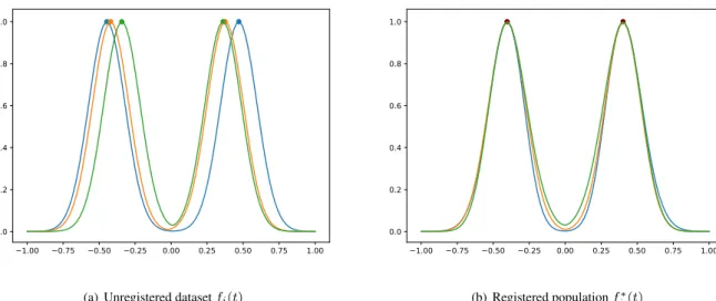
A landmark, or feature of a curve, is some characteristic that can be associated with a specific point of the domain. There are typically maximums, minimums or zero crossings points. For instance, the population shown in Figure2.10has two distinctive features, formed by the maximum points of each of the samples. 1.00 0.75 0.50 0.25 0.00 0.25 0.50 0.75 1.00 0.0 0.2 0.4 0.6 0.8 1.0
(a) Unregistered datasetfi(t)
1.00 0.75 0.50 0.25 0.00 0.25 0.50 0.75 1.00 0.0 0.2 0.4 0.6 0.8 1.0 (b) Registered populationfi∗(t)
Figure 2.10:Shift registration of a dataset
The landmark registration process will require, for each observationfi, the identification of the
va-lues{tij}Fj=1associated with each of theF features, which will be aligned to a common point{t∗j}Fj=1.
fi∗(t∗j) =fi(γi(t∗j)) =fi(tij). (2.6)
Not all sets of populations have differentiated characteristics of this type, moreover, by taking into account only a limited number of points the resulting alignments can become quite artificial, altering the internal structure of the samples. This will motivate us to build methods which use a global criterion for alignment and not just a discrete number of points.
2.2.4.
Pairwise and groupwise alignment
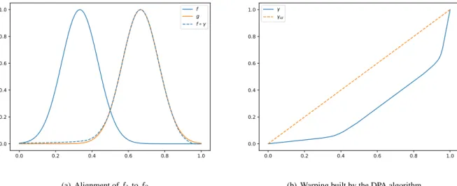
We will define the pairwise alignment problem [8] to deal with the registration problem of two fun-ctions using a global criterion.
Letf1, f2 ∈ F be functional observations of a general spaceF andE : F × F →R+ an energy
functional. The alignment problem may be understood as the search of a warping functionγ∗ which minimizes the energy between the two functions, i.e.,
γ∗= argmin
γ∈Γ
E[f1, f2◦γ]. (2.7)
When a warping γ∗ fulfills this property, we will say that f1 is registered to f2 ◦γ∗. In the Figure
2.11(a)it is shown an example where two functions have been registered using this approach.
0.0 0.2 0.4 0.6 0.8 1.0 0.0 0.2 0.4 0.6 0.8 1.0 f g f (a) Alignment off1tof2 0.0 0.2 0.4 0.6 0.8 1.0 0.0 0.2 0.4 0.6 0.8 1.0 id
(b) Warping built by the DPA algorithm
Figure 2.11:Pairwise alignment
To estimateγ∗, we will explore different paths that the reparameterization may take in a discretized grid, trying to minimize the energy term. This algorithm, described in deatil in [8], is called Dinamic
programming algorithm (DPA), because it makes use of dynamic programming techniques to search
2.2. Registration
the optimal path [12].
Given a set of functions{fi}ni=1⊂ F, the groupwise alignment problem will consist in the search of
warping functions{γi∗}n
i=1 ⊂Γto align each of the functions with the rest of them. To achieve this, we
will build a target functionµ, also called template, to which all the curves will be aligned. For instance, the cross-sectional mean of the functionsf¯= n1 Pn
i=1fican be used as target.
A possible choice for the energy term would be to takeE[f1, f2] = kf1 −f2k2L2 =
R
T(f1 −f2)2.
This criterion is not commonly used in practice because three problems will arise that will not make it adequate: the pinching effect, the lack of symmetry and the inverse inconsistency [13]. In what follows we provide a a short description of these issues.
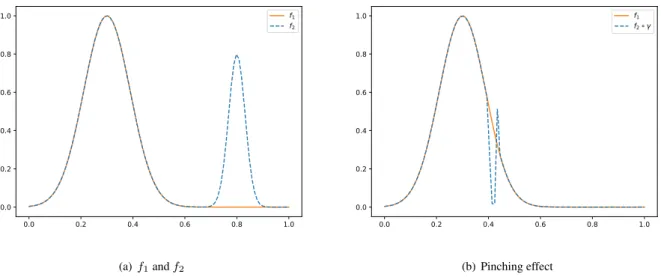
Pinching effect
The pinching effect can be observed when two functions without a perfect match are aligned, taking theL2 distance as energy. To minimize the energy termE in eqn. 2.7, the optimal solution will tend
to squeeze a region whose features make it difficult to align, until it disappears. Figure 2.12 shows the pinching effect on the registration of two functions. A part off2 is identical to f1 over [0, 0.6] and
completely different over the remaining domain. The optimal solution will tend to squeeze the second part off2, until it vanishes completely.
0.0 0.2 0.4 0.6 0.8 1.0 0.0 0.2 0.4 0.6 0.8 1.0 f1 f2 (a)f1andf2 0.0 0.2 0.4 0.6 0.8 1.0 0.0 0.2 0.4 0.6 0.8 1.0 f1 f2 (b) Pinching effect
Figure 2.12:Pinching force effect
Lack of symmetry
Letf1, f2 ∈ Fbe two functions that are aligned following the pairwise criterion (eqn.2.7). Generally,
if we apply a reparameterizationγ ∈Γto both functions, their distance will change, kf1◦γ−f2◦γk2= Z T (f1(γ(t))−f2(γ(t))|2dt= Z T |f1(s)−f2(s)|2 1 ˙ γ(γ−1(s))ds (s=γ(t)), (2.8)
in other words, the action ofΓoverF under theL2 metric is not by isometries.
ThereforeE[f1, f2]6=E[f1◦γ, f2◦γ]and consequentlyf1◦γ yf2◦γmay not be aligned. A direct
consequence of this issue will be the inverse inconsistency of the problem, because ofE[f1◦γ, f2]6= E[f1, f2◦γ−1]. It would be desirable that the transformation necessary to alignf1 tof2be the inverse
transformation to alignf2 tof1. The search of a more adequate energy for this problem will motivate
the Section2.3of this work.
2.2.5.
Amplitude phase decomposition
It is useful to quantify the amount of variability due to the phase and the amplitude, in order to understand the data and validate the registration procedure. For this purpose, in Kneip and Ramsay (2008) [14] it is developed an effective method for quantifying this variation once the data have been aligned.
Let {fi}Ni=1 be a set of functional observations, and {fi∗}Ni=1 = {fi ◦ γi}Ni=1 the corresponding
registered samples, andf¯,f¯∗the cross-sectional means. The Total Mean Square Error is defined as
MSEtotal= 1 N N X i=1 kfi(t)−f(t)k2= 1 N N X i=1 Z [fi(t)−f(t)]2dt. (2.9)
This error can be decomposed as MSEtotal = MSEamp +MSEphase. This decomposition allow
separate the variability due to the phase and the amplitude.
MSEamp =CR 1 N N X i=1 Z fi∗(t)−f∗(t)2 dt MSEphase= Z h CRf∗ 2 (t)−f2(t)idt (2.10)
WhereCRis a constant related with the covariance betweenγ˙iand(fi∗)2. From this decomposition
it is possible to define the square error multiple correlation index, which indicates the proportion of the variation due to the phase explained by the registration process. This index is defined as
R2= MSEphase
MSEtotal . (2.11)
For instance, by quantifying the alignment of the dataset of the Figure2.8, we get a value of
R2 = 0,99, which indicates that the99 %of the variability it is produced by the phase.
2.3. Elastic methods in functional data analysis
2.3.
Elastic methods in functional data analysis
As discussed in previous chapter, the variability in functional data may come from the continuous structure of its domain. This problem does not appear exclusively in functional data analysis, other fields such as shape analysis or computer vision should deal with this kind of variability.
In the classical approach, phase variation is separated in the registration of the data, as a prepro-cessing step. However, in the elastic analysis approach the separation of the two sources of variability is incorporated as a fundamental part of the analysis. The termelastic comes from the fact that we will allow deformations of the domain of the functions throughout the analysis.
In Srivastava et. al. (2011) present in [15] a novel framework to treat this approach using the Fisher-Rao metric. Although this framework covers a wide variety of topics, such as classification, regression or functional component analysis [16], in this chapter we will focus on the part concerning the so-called elastic registration of functional data. For that, we will follow the explanation outlined on chapters 1, 3, 4, and 8 of the book Functional and Shape Data Analysis [8] and the implementation in the R-package
fdasrvf [17].
2.3.1.
Fisher-Rao metric
As introduced in Section2.2.4, the use of the metricL2for the pairwise alignment of functions leads
to a series of difficulties, which make it unsuitable for this problem. This is why we will use differential geometry techniques to find a suitable metric. In particular, given two functionsf1,f2 andγ ∈ Γ, we
look for a metric that remains invariant to warpings in the domain, i. e.,d(f1, f2) =d(f1◦γ, f2◦γ).
For this purpose we will use the Fisher-Rao metric. This Riemannian metric was introduced in 1945 by C. R. Fisher in a version on the space of probability distributions. In our case we will use a non-parametric version, slightly different from the original one, defined on the space of signed measures. This metric plays a very important role in information geometry, and it is the only metric that possesses this property of invariance to warpings in the domain [18].
γ
(t)
υ
x
T
x
M
M
A Riemannian metric is an application that assigns an inner product at each point of variety on its tangent space that varies smoothly from point to point. This will give us local notions of angles, length of curves or volumes.
The tangent space of a manifold facilitates the generalization of vectors to general manifolds, since one cannot simply subtract two points to obtain a vector that gives the displacement of the one point from the other. The tangent space of a pointxin a general manifoldM, denoted asTxM, is made up
of the velocities atxof all the paths of the variety passing through the point. For example, in the Figure
2.13is shown a manifoldM inR3. This velocities of the path are tangent vectors to the curve. In this
case the tangent spaceTxM made up of all these vectors is a plane.
In our case the manifold will be formed by the set of absolutely continuous functionsF, that is, those functions whose derivative exists a.e. and belongs to the space of square integrable functionsL2. And the path between points of F may be understood as smooth deformations of the functions. We will endowF with the Fisher-Rao metric.
Letf ∈ F andv1, v2 ∈Tf(F), the Fisher-Rao metric is defined as
hhv1, v2iif = 1 4 Z 1 0 ˙ v1(t) ˙v2(t) 1 |f˙(t)|dt, (2.12)
wherev˙ denotes the derivative ofv.
Using this local notion of inner product, we will be able to calculate the length of α(τ) ⊂ F, a differentiable path in our manifold as
L[α] =
Z 1
0
hhα˙(τ),α˙(τ)iiα(τ)dτ. (2.13)
This allows us to define the distance between two points of the manifoldf1, f2 ∈ F as the length of
the geodesic path, or shortest path, which connectsf1andf2,
dF R(f1, f2) = ´ınf
α:[0,1]→F,α(0)=f1,α(1)=f2
L[α]. (2.14)
This path is the shortest smooth deformation between f1 and f2. Figure 2.14(a) illustrates some
steps in the deformation between f1 and f2. Finding this geodesic path directly is computationally
unapproachable, for this reason we will introduce the Square Root Slope Funcion (SRSF) transform, which simplifies this computation.
Givenf ∈ F, itsSRSFis defined as SRSF{f}= sgn ( ˙f) q
|f˙|. To simplify notation, in the subse-quent sections, we will denote theSRSFof a functionfi∈ F asqi.
1Derivative work: McSush. Original uploader: TN at German Wikipedia. [Public domain]
2.3. Elastic methods in functional data analysis 2.0 1.5 1.0 0.5 0.0 0.5 1.0 1.5 2.0 0.0 0.2 0.4 0.6 0.8 1.0 f1 f2
(a) Five steps of the geodesic path betweenf1andf2
2.0 1.5 1.0 0.5 0.0 0.5 1.0 1.5 2.0 2.0 1.5 1.0 0.5 0.0 0.5 1.0 1.5 2.0 q1 q2 (b) SRSF of the path
Figure 2.14:Geodesic path inFand the corresponding SRSF’s
Under this transformation, the Fisher-Rao metric becomes the usual metric inL2, so that the
distan-ce between two functions will be calculated using the distandistan-ceL2 of their corresponding SRSF’s, i.e., dF R(f1, f2) =kq1−q2kL2. A proof of this result is included in appendixA.2.
Taking advantage of this characterization we will take our functions to the SRSFs space to perform the analysis efficiently, and then transform the result to the original space. This can be done because theSRSF defines a map up to constant between F and the space of SRSFs with the L2 metric. A
consequence is that the computation of geodesics shown in2.14becomes in a straight line between SRSFs,α(τ) = (1−τ)q1+τ q2 0≤τ ≤1.
Givenγ ∈Γ, the SRSF off ◦γis
SRSF{f◦γ}= sgn( ˙f ◦γ) q
|f˙◦γ|pγ˙ = (q◦γ)pγ.˙ (2.15)
To simplify the notation, theSRSFof this composition is denoted by(q, γ). Using this fact, we can proof that the action ofΓon F is an action by isometries, i.e, givenf ∈ F andγ ∈Γthe composition
f ◦γ preserves the metric. A proof of this result is given in the appendix A.2. Figure 2.15 shows a diagram with the action of the composition in the different spaces.
z
1z
2z
1e
iθz
2e
iθT
e
iθ1e
iθ2C
/
T
[
z
1]
[
z
2]
T
e
iθne
iθ¯T
e
i(θn−θ¯)1
f
q
f
◦
γ
(
q, γ
)
SRSF action on F action on L2 SRSF Figure 2.15:Action ofΓ2.3.2.
Amplitude and phase spaces
Due to the properties of the Fisher-Rao metric, we can formally decompose the distance between two functions ofF into the part due to phase and amplitude.
z1
z
2z1e
iθz
2e
iθT
e
iθ1e
iθ2C
/
T
[z
1]
[
z
2]
T
e
iθne
iθ¯T
e
i(θn−θ¯)1
f
q
f
◦
γ
(
q, γ
)
SRSF action onF action on L2 SRSF1
Figure 2.16:Rotation in complex planeFirstly, it is useful to consider and analogy with the rotations on the complex plane, to understand the role by the phase and the amplitude in the manifoldF.
Let z1, z2 be two points in C, as it is illustrated in the Figure 2.16, when a rotation on the plane
is applied the distance betweenz1 andz2 remains invariant, i.e., it is an action by isometries, as the
reparameterizations on our manifold.
The variability between two vectors in the plane is completely specified by the angle between them, which will play the role of the phase in our space, and the difference of their modules, which will be equivalent to the distance between the vector once aligned.
z1 z2 z1eiθ z2eiθ T eiθ1 eiθ2 C/T [z1] [z2] T eiθn eiθ¯ T ei(θn−θ¯) 1 f q f◦γ (q, γ) SRSF action onF action onL2 SRSF 1 (a) Angle between vectors
z1 z2 z1eiθ z2eiθ T eiθ1 eiθ2 C/T [z1] [z2] T eiθn eiθ¯ T ei(θn−θ¯) 1 f q f◦γ (q, γ) SRSF action onF action onL2 SRSF 1 (b) Distance inC/T
Figure 2.17:Phase and amplitude in the complex plane
This distance of the vectors aligned may be understood as a distance in the quotient spaceC/T,
whereT is the unit circle, which it is isomorph to the group of rotations in the planeSO(2). In this
2.3. Elastic methods in functional data analysis
quotient space we will define the equivalence classes[z] ={zeiθ :θ∈[0,2π]}.
In the case of our manifold, letq∈L2be aSRSF. We will define its orbit underΓas
[q] ={(q, γ) :γ ∈Γ}, in other words, it is the set of reparameterizations associated to q. In the Figure
2.18(a) it is shown some reparameterizations associated to a function of F and their corresponding
SRSF’s in2.18(b). 1.00 0.75 0.50 0.25 0.00 0.25 0.50 0.75 1.00 0.00 0.25 0.50 0.75 1.00 1.25 1.50 1.75 f i (a) f◦γi 1.00 0.75 0.50 0.25 0.00 0.25 0.50 0.75 1.00 3 2 1 0 1 2 3 (q i) i (b)(q, γi)
Figure 2.18:Functions in the same orbit
We will denote amplitude spaceA =L2/Γto the set of these orbit. In this space the phase variation
is incorporated within equivalence classes, while the amplitude variation appears across equivalence classes, as in the analogy with the complex plane. We will endow the space with the elastic metric, defined as
da([q1],[q2]) = ´ınf
γ1,γ2∈Γ
(k(q1, γ1)−(q2, γ2)k), (2.16)
To quantify the other source of variability, we will define the phase space, which will denoted as
Γ = {γ : [0,1] → [0,1] : γ is a boundary-preserving diffeomorphism}, for which the natural distance will be given by the Fisher-Rao metric.
Letγ ∈Γbe a warping function. Under the Fisher-Rao metric, the norm of suchγ is 1, thus kγk2Γ=kSRSF(γ)k2L2 =kγ˙k2 L2 = Z 1 0 p ˙ γ(t)pγ˙(t)dt= Z 1 0 ˙ γ(t)dt=γ(1)−γ(0) = 1. (2.17)
The SRSFtransform is an isometry between Γ and the unit sphere in L2, also known as Hilbert
SphereS∞={ψ∈L2:kψkL2 = 1}. To calculate distances inΓwe will apply this transformation which
Letγ1, γ2 be inΓandψ1= √ ˙ γ1, ψ2= √ ˙
γ1be theirSRSF, their distance inΓwill be given by dphase(γ1, γ2) =dψ(ψ1, ψ2) = cos−1 Z 1 0 ψ1(t)ψ2(t)dt . (2.18)
This result is analogous to the rotations in the plane, where the cosine of the angle between two unit vectors will be given by the inner product. If we apply a rotation to two vectors, their angle remains invariant, in our case the phase distance will be invariant to common reparameterizations due to the properties of the Fisher-Rao metric.
Letf1, f2 be functions inF, their relative phase is defined as (γ1∗, γ2∗) = argmin
γ1,γ2∈Γ
k(q1, γ1)−(q2, γ2)k ∈Γ×Γ. (2.19)
Thus allow us to calculate the phase variability between them, as a generalization of the notion of an angle. The phase distance between these functions is the distance of their relative phasedphase(γ1∗, γ2∗).
Alternatively, the properties of the metric can be used to define the relative phase depending on a single warping,γ12∗ = argmin
γ∈Γ
k(q1, γ)−q2k,which is quivalent to setγ2∗ to the identity in2.19.
2.3.3.
Pairwise alignment
The Fisher-Rao metric allow us to formulate a suitable criterion for the pairwise alignment problem, as presented in Section2.2.4, that avoids all the problems associated with the metricL2.
Givenf1, f2 ∈ F, to registerf1 tof2 the Fisher-Rao distance will be minimized as energy termE
(see eqn.2.7), i.e., the warping used in the alignment will be
γ∗ = argminγ∈ΓdF R(f1◦γ, f2) = argminγ∈Γk(q1, γ)−q2kL2. (2.20)
The energy used to align the functions in Figure2.11(a) is actually this quantity. SinceE[f1, f2] = E[f1◦γ, f2◦γ], the warping used to registerf1◦γ tof2◦γ will be the same as in the previous case.
Because of this property, our problem will have inverse consistency, since
E[f1◦γ, f2] =E[f1◦γ◦γ−1, f2◦γ−1] =E[f1, f2◦γ−1], (2.21)
so that the warping needed to registerf2tof1isγ∗−1. In addition, the so-called pinching effect will
not appear, due to the term√γ˙ that is present in the criterion to minimize.
2.3. Elastic methods in functional data analysis
2.3.4.
Karcher means
In descriptive statistics, given a set of random points{xi}Ni=1 ⊂Rn, the sample meanx¯= N1
PN
i=1xi
is used to estimate the central tendency of the data. The mean is the quantity that minimizes the sum of square distances.
In the functional case, the mean function will have this property thus if {fi}Ni=1 ⊂ L2 is a set of
functional observations, their meanf¯(t) = N1 PN
i=1fi(t)will minimizePNi=1kfi−f¯k2L2.
We are interested in extend this idea to general metrics spaces. Let(X, d) be a metric space and {xi}Ni=1random points inX. The Fréchet variance of a pointp∈Xis defined asΨ(p) =
PN i=1d2(p, xi). 1.00 0.75 0.50 0.25 0.00 0.25 0.50 0.75 1.00 0.0 0.5 1.0 1.5 2.0 2.5
(a) Dataset of unimodal samples
1.00 0.75 0.50 0.25 0.00 0.25 0.50 0.75 1.00 0.0 0.2 0.4 0.6 0.8 1.0
1.2 cross-sectional meanelastic mean
(b) Usual mean and Karcher mean onA
1.00 0.75 0.50 0.25 0.00 0.25 0.50 0.75 1.00 0.0 0.5 1.0 1.5 2.0 2.5
(c) Ranked by elastic distance
1.00 0.75 0.50 0.25 0.00 0.25 0.50 0.75 1.00 0.0 0.5 1.0 1.5 2.0 2.5
(d) Ranked by phase distance
Figure 2.19:Karcher mean of dataset
The Fréchet mean of these random points will be defined as the element m ∈ X which globally minimizes the Fréchet Variance. If this global minimum does not exist, we will call Karcher means to the points that locally minimizes the varianceΨ(p), i. e.,
m= arg m´ın p∈M N X i=1 d2 p, x˙i (2.22)
These Karcher means are adapted to the metrics used in the analysis. For this reason they can better capture the geometry of our problem than usual mean, as it is shown in the Figure 2.19(b), where it is used a Karcher mean onA. The dataset shown in2.19(a)contains Gaussian-like samples, however the usual mean of Figure2.19(b)is not able to reflect this shape, unlike the Karcher mean in
A.
As an example of the behavior of these means with different metrics, the centrality of an observation in a dataset can be measured using its distance to the Karcher mean. In the Figure2.19it is used this idea to rank a dataset of unimodal samples. Reddish colors indicate higher centrality of a sample, i.e., a smaller distance to the mean, and lighter colors indicates outlier samples. In the Figure2.19(c)it is used the amplitude distance, and their corresponding Karcher mean. We can observe that the location of the mode in a sample does not affect its centrality, in contrast to the phase distance, as it is shown in the Figure2.19(d).
2.3.5.
Elastic registration
In this section we will define a procedure, which will be called elastic registration, to perform a groupwise alignment of a dataset under this framework. A target function will be created, called the elastic mean, to which all samples will be aligned later, as discussed in Section2.2.4.
Let{fi} ⊂ F be a dataset of functions to register andqi their corresponding SRSFs. Firstly we will
compute their Karcher mean inA, defined as
[µq] = arginf [q]∈A n X i=1 da([q],[qi])2. (2.23)
The bracket notation[µq]is used to emphasize the fact that it is an orbit in a quotient space. We will
need a criterion to select a particular element of this orbit, for that reason we will define the center of the orbit as the elementµ˜q ∈[µq]such that the relatives phasesγi∗ betweenqi and[µq]have as Karcher
mean the identity.
F
L
2
A
q
i[
q
i]
˜
µ
fµ
˜
q2
Figure 2.20:Scheme of the elastic registration procedure.
2.3. Elastic methods in functional data analysis
We will select an arbitrary elementµq of[µq]to which we will calculate the corresponding warping
functions to align the set of SRSFs, i.e.,γi = arginfγ∈Γkq˜−(qi, γ)k. Then, we will compute the Karcher
mean of{γi}, denoted asγ¯, in the phase space. The center of the orbit will be µ˜q = (µq,¯γ−1). The
mean of the relative phases with respect to the center of the orbitµ˜q, will be the identity, thus
arginfγ∈ΓdF R(γi◦γ¯−1, γ) = arginfγ∈ΓdF R(γi◦γ¯−1◦¯γ, γ◦γ¯) = arginfγ∈ΓdF R(γi, γ◦¯γ) =γid. (2.24)
Finally, we will construct the template to which the samples will be aligned, called elastic mean,
˜
µf = N1 PNi=1fi(0) + Rt
0µ˜q(s)|µ˜q(s)|ds, which is the pullback of µ˜q to the original space F. In the
Figure2.21may be observed the result of the registration of the berkeley growth curves of the Figure
2.6. 2 4 6 8 10 12 14 16 18 age (year) 0.0 2.5 5.0 7.5 10.0 12.5 15.0 17.5 20.0 he igh t/ ag e ( cm /ye ar )
Figure 2.21:Elastic registration of the Berkeley velocity curves
An important property of the elastic mean µ˜f is that given a dataset{cif(γi(t)) +ei}ni=1, where
{γi}ni=1have as Karcher mean inΓthe identity andciandei are positive constants with mean1and0
respectively, thenµ˜f is a consistent estimator off [15].
2.3.6.
Restricting elasticity
Sometimes it is necessary to control the amount of elasticity during the registration process, for this purpose it is possible to add a penalty termR(λ) to the elastic distance2.16. Let q1, q2 ∈ L2 be two
SRSFs andλ >0, we will define the penalized elastic distance as
dλ(q1, q2)≡´ınf γ∈Γ kq1− q2◦γ p ˙ γ2+λ p ˙ γ−1k2(1/2). (2.25)
0.0 0.2 0.4 0.6 0.8 1.0 0.0 0.2 0.4 0.6 0.8 1.0 f g
(a) Registration off1tof2with a penalty term
0.0 0.2 0.4 0.6 0.8 1.0 0.0 0.2 0.4 0.6 0.8 1.0
(b) Warping used in the alignment
Figure 2.22:Penalized elastic registration with different values ofλ
Once the registration process of our data has been completed, we can proceed to another parts in the analysis of the data. Regression and classification are two of the most important problems in statistics, and therefore inFDA. Among the models to address these tasks are the nearest neighbors estimators, which can be generalized directly to functional data. In the following section is made a brief overview of these estimators.
2.4.
Nearest neighbors
After representing the data in functional form, and preprocessing it to quantify and reduce its variabi-lity, it may be interesting to study the relationship between various functional variables. As in Multivariate Statistics and Machine Learning,FDAwill deal with the regression and classification problems, but in the case where some of the data are of a functional nature.
Inclassification, or more precisely supervised classification, the category or population to which an
observation belongs is studied, using a set of data whose category is known. For example, predicting the climate type of a region from its temperature curves is a functional classification problem.
In regressionis studied the existing relation between two or several random variables. Instead of
predicting a class label, as in classification, regression models are created to predict another variable, called dependent variable or response, from one or more known variables. In the case of functional prediction we must make a distinction that does not appear in classical statistics between two cases, when the response to predict is an scalar quantity or is also a functional datum. For instance, the prediction of the total precipitation of a region from its temperature curves is a regression problem with scalar response, as opposed to the case with functional response, in which is predicted the precipitation curves from the temperatures. Among the models most used for these two problems can be found the nearest neighbors estimators.
2.4. Nearest neighbors
The Nearest Neighbors (NN) estimators are a family of methods widely used in Statistics and
Machine Learning, in problems of classification or regression, among others. These estimators are based on the idea of neighborhood, using the notion of distance, so that it is made a local estimation of the density of the data. Although in their classic version they are used with sets of vectors, their ideas work in the same way in general metric spaces [19], as the functional ones we consider in this work.
Let(F, d)be a metric space and(fi, Yi)i≤i≤na training set with their respective labels or responses.
To estimate a datumx, either for classification or prediction of its response, firstly, it will be necessary to find the elements of the training set closest to this datum, which will form its neighborhood, denoted ask(x).
There are two variants of these methods. In the first one, consisting of K-Nearest Neighbors (KNN)
estimators, it is taken as neighborhood the k closest elements tox, i. e., if the training pairs are re-indexed as (f(i), Y(i)) 1 ≤ i ≤ n so that the f(i)’s are re-arranged in increasing distance from x,
d(x, f(1))≤d(x, f(2))≤ · · · ≤d(x, f(n)), thenk(x) ={f(i) : 1≤i≤i≤k}. 0.0 0.2 0.4 0.6 0.8 1.0 1.0 0.5 0.0 0.5 1.0
(a) K-nearest neighbors
0.0 0.2 0.4 0.6 0.8 1.0 1.0 0.5 0.0 0.5 1.0 (b) Radius-nearest neighbors
Figure 2.23:Neighborhoods using distanceL∞
In the second variant, less used in practice, consisting of the radius neighbors estimators, the neigh-borhood contains the samplesfi in the ball of radius r centered inx, i.e.k(x) = {fi : d(fi, x) ≤ r}.
For instance, if we use the distanceL∞, we may visualizek(x)as the set of all functions within a band
of radius r aroundx. In the figure 2.23 there are shown the neighborhoods with these two different approaches.
In practice, for the construction of the neighborhoods, the simplest solution is to perform a linear search, calculating the distances betweenxand all the elements of the training set. The naïve approach of the linear search may be improve using data structures based on spatial indexes, such as ball trees [20]. However, the best nearest-neighbors data structure for a given application will depend on the dimensionality, size, and underlying structure of the data.
2.4.1.
Classification
In the classification problem, the samples of the training set fi are associated to the labels Yi
corresponding to their class. Given a datumx, a new label is predicted using the majority class among its neighbors, so that the predicted class will be
ˆ Y = argmax j X fi∈k(x) 1{Yi=j}. (2.26)
It is possible to make a weighting vote, so that the closest neighbors will have a greater weight, for example, usingwi = 1/d(fi, x), so that the resulting label will beYˆ = argmax
j P
fi∈k(x)wi1{Yi=j}.
2.4.2.
Regression
In the regression problem, each of the training samplesfihave a responseYiassociated with them.
This response can be either scalar or functional, although the way to proceed will be similar.
In both cases, it is necessary to select the responses associated with the elements of the neighbor-hoodk(x), which will be used to predict the response of the datumx.
In the scalar response case, a weighted average of the neighbors’ responsesYiis used, so that the
prediction will be calculated as
ˆ
Y = X
(fi,Yi):fi∈k(x)
wiYi, (2.27)
whereP
wi= 1. which may be chosen based on distance or uniformly.
In the case where the responses are also functional data, the predicted response is constructed in a similar way as in the previous case, using a weighted average of functions, or a centroid, such as the Karcher means presented in Section2.3.5.
During this chapter we have focused on making a brief description of the mathematical concepts used in this work. The aim of this work was to include all these concepts as functionalities in the scikit-fdapackage. The next chapter summarizes the design decisions followed for this task, the technologies used for it and the methodologies used for this purpose.
3
D
esign and development
In this chapter we will make a brief summary of the technologies and development followed during this work, in which the mathematical concepts discussed throughout the Section2have been incorpo-rated inscikit-fda. On the one hand, we will discuss the requirements and design raised in development. During the design stage it has been special emphasis on creating anAPIsimilar to the packages of the
scipy[22] ecosystem, allowing the integration of functionalities of some of these libraries. This facilitates
the use of the package to developers and researchers who already know this ecosystem, widely used for Statistics and Machine Learning in Python. Because of these features, and to allow a wider diffusion of the package, it was decided to develop the project as anscikit, which are open source packages for scientific computing in Python. To promote this diffusion, during this work has been managed the creation of a logo, used as a symbol of the project. This logo is shown in the Figure3.1.
Figure 3.1:Scikit-fda logo
On the other hand, this chapter presents the technologies used for the development of the package, which currently supports Python 3.6 and 3.7. Among the tools used in this development has been used
git, to perform version control. This tool has allowed the communication of the team involved in the development, and the integration of a Continuous integration (CI) system for the execution of tests and generation of online documentation.
In addition, there is a brief summary of the methodology followed in this work, which had to be integrated together with the work of a team. For this integration it has been necessary a great com-munication, carrying out weekly meetings throughout the year. This communication has been possible thanks to the version control system, which has allowed revisions of the work among the members of
the development team. Due to the open-source nature of the project, these revisions and the code are publicly available. For this reason special emphasis has been placed on the quality of the code, which will be maintained and used by multiple developers throughout the life of the project.
3.1.
Analysis
As mentioned above, the scikit-fda project started in 2017, at which time an analysis of the re-quirements of the package was made [5]. These requirements are still in effect today, some of them are:
• The software developed has to be a Python package.
• It has to be an open-source project.
• The software must follow Python standards defined in PEP 8 and PEP 257.
• Documentation has to be intended for a very general audience.
• The project has to include and extensive test bench of unit test and continuous integration mechanism.
In addition to the original ones, three new requirements have been formulated:
• The software should be cross-platform and the mechanism of continuous integration should run the test bench in
the main operating systems, that is, Linux, MacOs and Windows, as well as different Python versions supported.
• API should be similar, as far as possible, to thenumpy [21] ,scipy andscikit-learn ones, allowing whenever
possible the use of their functionalities with the objects of the software developed.
• The documentation should contain examples showing different functionalities.
3.2.
Design
Originally the package was structured around two classes, FDataGrid and FDataBasis, designed for each of the main data representations of the data and consisted of four modules with basic statistics, operations and methods to perform kernel smoothing.
Due to the expansion of the project, the package has been completely restructured, with a more hierarchical structure. Figure3.2shows a diagram of the main modules of the package. Darker colors in the figure represent a more advanced stage of development of the modules. The following subsections summarize, in general terms, the functionalities incorporated and design changes made during this work. A more detailed description of the functions and classes developed may be found in AnnexC, or in the online documentation, available atfda.readthedocs.io.
3.2. Design
8
exploratory analysis representation preprocessing
statistical inference machine learning
scikit-fda
Figure 3.2:Map of scikit-fda [6]
3.2.1.
Representation module
Therepresentationmodule includes general functionalities for the representation of functional data
and classes for processing this data using a object-oriented paradigm. There were two classes,
FDa-taBasis and FDataGrid, to represent the data in basis or discretized form, as it was explained in the
indroduction of the Chapter 2. These classes contain common functionalities. In order to unify these functionalities, an abstract class calledFData has been created, from which the previous ones inhe-rit. This class implements methods for the evaluation of the data as functions and its plotting. Aside from methods for the composition of functions or operations between them. The method created for the evaluation of functional data inFDataallows its evaluation as vectors of functionsf = (f1, f2, . . . , fn)0
wherefi :Rd→Rm, using a similar syntax to the mathematical notationf(t). It is also allowed to call
these functions in a vectorized way with multiple values, so that
f((t1, t2, . . . , tk)) = f1((t1, t2, . . . , tk)) f2((t1, t2, . . . , tk)) .. . fn((t1, t2, . . . , tk)) = f1(t1) f1(t2) . . . f1(tk) f2(t1) . .. f2(tk) .. . . .. ... fn(t1) fn(t2) . . . fn(tk) (3.1)
wheret1, t2, . . . tk are the points of evaluation inRd. For example, the code3.1shows the creation
of a set of three random samples defined in[0,1]. These samples are packed in aFDataobject using a discrete representation. The they are then evaluated at0,0,5and1.
>>> from s k f d a . d a t a s e t s i m p o r t m a k e _ s i n u s o i d a l _ d a t a >>> >>> f = m a k e _ s i n u s o i d a l _ p r o c e s s ( n_samples =3 , s t a r t =0 , s t o p =1) >>> f ( [ 0 , 0 . 5 , 1 ] ) .round( 3 ) a r r a y ( [ [−0 . 6 7 7 , 0 . 3 6 8 , −0.372] , [ 0 . 7 0 2 , −0.717 , 0 . 7 6 5 ] , [−0.8 , 0 . 4 0 5 , −0 . 7 0 3 ] ] )
The evaluation method separates the evaluation points tj into two sets, depending on whether
they are inside or outside the domain range of the functions. The points within the domain range are passed to the evaluator, defined by the type of representation, to its evaluation, which will depend on the implementation of the representation. In the discrete representation it is used interpolation to this purpose.
A submodule called interpolation has been created with different interpolation methods, used in the class FDataGrid as evaluator. In this module may be found the SplineInterpolation class, which implements the different interpolation techniques explained in the Section2.1.
In addition, FData objects have an extrapolator, to which points outside their domain are passed during the evaluation. It was created a submodule calledextrapolationwith different extrapolators used in this task, in which they have included the classesPeriodicExtrapolation, to extend the domain perio-dically,BoundExtrapolation, to use the values of the limits orFillExtrapolation, to return a fixed value.
Once the data is in functional form using an FData object, it is possible to use the rest of the functionalities of the package, such as the registration methods or the models for regression and clas-sification.
3.2.2.
Preprocessing module
In the preprocessing module a specific module calledregistrationhas been created to deal with the registration of the data using the techniques explained throughout the sections2.2and2.3. Among the functions incorporated in this module areshift_registration, for registrations using shifts,
landmark_registration, to employ known landmarks, orelastic_registrationwith the algorithm detailed in
Section2.3.5. In addition, this module contains functions for the treatment of warpings functions among other useful processes during the registration phase. To ensure the efficiency of the algorithm used in the pairwise alignment (eqn.2.7), it was implemented usingC, which is called by the Python package throughCython.
All the registration methods have been designed to receive anFDataobject and return another one containing the registered samples, which can be used with other functionalities of the package, such as the classification or regression models included in the machine learning module.
3.2.3.
Machine learning module
The package contains a module with tools for machine learning. This module is divided into three submodules calledclassification,regression andclustering. Models for data classification and regres-sion have been incorporated using the