ANALYSIS OF LOAD MATCH AND GRID
INTERACTION INDICATORS IN NET ZERO
ENERGY BUILDINGS WITH
HIGH-RESOLUTION DATA
A report of Subtask A
IEA Task 40/Annex 52 Towards Net Zero Energy Solar Buildings
March 2014
Title Analysis Of Load Match and Grid Interaction Indicators in NZEB with High-Resolution Data
Coordination Jaume Salom
Catalonia Institute for Energy Research, IREC Jardins de les Dones de Negre, 1
08930 Sant Adrià de Besòs (Barcelona) Spain
Contact: [email protected] Project IEA Task 40 / Annex 52 Task / Subtask Subtask A
Authors Jaume Salom, IREC, Spain
Anna Joanna Marszal, Aalborg University, Denmark
José Candanedo, CanmetENERGY, Natural Resources Canada, Canada Joakim Widén, Uppsala University, Sweden
Karen Byskov Lindberg, Norwegian University of Science and Technology, Norway Igor Sartori, SINTEF, Norway
Contributors Usman Ijaz Dar, NTNU, Norway Ala Hasan, VTT, Finland
Björn Berggren, Lund University, Sweden Søren Østergaard Jensen, DTI, Denmark Francesco Guarino, Università di Palermo, Italy Davide Nardi Cesarini, AEA – Loccioni, Italy Andreas Molin, Linköping University, Sweden Eike Musall, University of Wuppertal, Germany Karsten Voss, University of Wuppertal, Germany Maria Leandra González Matterson, IREC, Spain
Selvam Valliappan, National University of Singapore (NUS), Singapore Sent to review October 2013
Index
EXECUTIVE SUMMARY ___________________________________________ 5
ACRONYMS _____________________________________________________ 9
1
INTRODUCTION ____________________________________________ 10
2
TECHNICAL FRAMEWORK ___________________________________ 13
2.1 NATIONAL / REGIONAL ENERGY SYSTEM 13
2.2 ELECTRICITY DISTRIBUTION GRIDS 15
2.2.1 DISTRIBUTION GRID STRUCTURE, OPERATION AND PLANNING 15 2.2.2 HOSTING CAPACITY FOR DISTRIBUTED GENERATION 16 2.2.3 RELEVANT HIGH-RESOLUTION INDICATORS FOR NET ZERO ENERGY BUILDINGS 20 2.2.4 REQUIRED ELECTRICAL PEAK LOADS FOR LOW-VOLTAGE SUPPLY 21
2.3 BUILDING DESIGNERS / OWNERS PERSPECTIVE 22
3
LMGI INDICATORS __________________________________________ 23
3.1 INTRODUCTION 23
3.2 TERMINOLOGY 24
3.3 LOAD MATCH INDICATORS 28
3.3.1 LOAD MATCH INDEX 28
3.3.2 LOAD COVER FACTOR AND SUPPLY COVER FACTOR 28 3.3.3 DIFFERENCE BETWEEN LOAD COVER FACTOR AND LOAD MATCH INDEX 31
3.3.4 LOSS OF LOAD PROBABILITY 33
3.4 GRID INTERACTION FACTORS 34
3.4.1 PEAK POWER GENERATION/EXPORTED 34
3.4.2 PEAK POWER LOAD/DELIVERED 34
3.4.3 GENERATION MULTILPLE 34
3.4.4 DESIGN RANGE 35
3.4.5 NET EXPORTED VALUES AND RANGES 35
3.4.6 CAPACITY FACTOR 35
3.4.7 DIMESIONING RATE 36
3.4.8 CONNECTION CAPACITY CREDIT 36
3.4.9 PEAKS ABOVE CERTAIN LIMIT 37
3.5.3 GRID CITIZENSHIP TOOL 38
3.5.4 EQUIVALENT HOURS OF STORAGE 39
4
CASE STUDIES _____________________________________________ 40
4.1 MONITORED BUILDINGS 40
4.1.1 MB1 AND MB2-FLAMINGO HOUSE -DENMARK 42
4.1.2 MB3-ENERGY FLEX HOUSE -DENMARK 43
4.1.3 MB4- ZEB@BCAACADEMY -SINGAPORE. 44
4.1.4 MB5-LEAF HOUSE -ITALY 45
4.1.5 MB6–CHPWUPPERTAL-GERMANY 46
4.1.6 MB7–FINNÁNGEN HOUSE -SWEDEN 47
4.2 SIMULATED BUILDINGS 48 4.2.1 SB1 AND SB2 -DENMARK 49 4.2.2 SB3 AND SB4-GERMANY 50 4.2.3 SB5–FINLAND 51 4.2.4 SB6-NORWAY 52 4.2.5 SB7–SPAIN 53 4.2.6 SB8 AND SB9-SWEDEN 53
4.2.7 SIMULATED BUILDINGS: ADDITIONAL INFORMATION 54
5
RESULTS AND DISCUSSION _________________________________ 55
5.1 OVERVIEW OF ENERGY BALANCE 55
5.2 LOAD MATCHING FACTORS 63
5.3 GRID INTERACTION FACTORS 73
5.3.1 GRID INTERACTION FACTORS RELATED TO GRID CONNECTION CAPACITY (EDES) 73
5.3.2 PEAKS ABOVE LIMIT /BARRIER 91
5.3.3 GRID INTERACTION INDEX 92
5.3.4 GRID CITIZENSHIP TOOL 93
5.4 RESULTS USING HOURLY OR SUB-HOURLY RESOLUTIONS 95
6
CONCLUSIONS AND FUTURE RESEARCH WORK ________________ 97
6.1 LOAD MATCH FACTORS 97
6.2 GRID INTERACTION FACTORS 98
Page 5 of 102
EXECUTIVE SUMMARY
A Net Zero Energy Building (Net ZEB) is succinctly described as a grid-connected building that generates as much energy as it uses over a year. The “Net Zero” balance is attained by applying energy conservation and efficiency measures and by incorporating renewable energy systems. The main objective of this report is to analyze the usefulness and relevance of proposed Load Match and Grid Interaction (LMGI) for Net Zero Energy Buildings. The methodology is based in the analysis of available high-resolution data (mainly hourly) both from simulated and monitored Net ZEBs (Net Zero Energy Buildings) or nZEB (nearly Zero Energy Buildings). The central question is to find a limited set of indicators which provide relevant information to building owners, local grid Distribution System Operators (DSO) when information from building simulations are available at design stage.
The first two sections of the report introduces why load matching and grid interaction are key aspects to be analysed in Net ZEBs together with the fulfilment of the yearly energy balance between on-site generation and buildings load. Buildings will play a significant role as part of an energy system based on DER – Distributed Energy Resources. Section two analyses the subject from several perspectives from the operators of national energy grids to the building owners and users. More details and references to previous studies are given when the conditions for the distribution grids are discussed, as the buildings are mostly connected to the medium and low-voltage grid. Analysis concludes that an accurate analysis will need detailed information of the grid topologies, which in most of the cases is not the case when Net ZEBs are being planned. Also, it is highlighted that grid interaction is an aspect that should be analysed in the framework of urban planning (at the cluster of buildings level) more than at individual building level.
Page 6 of 102
The third chapter of the report defines the load match and grid interaction indicators that should be computed with the case studies, together with describing the terminology. This is defined in coherence with the framework for Net ZEBs definition established in this current IEA Task. The indicators are computed in sixteen case studies. Seven of them are based on monitored buildings which are individual houses in Nordic countries (Sweden and Denmark), block of flats in Germany and Italy (with a CHP and GSHP with PV systems, respectively) and an office building in Singapore. Monitored data are from a complete year with different details of time resolution (from one minute to one hour). The nine case studies with simulated data use one-hour time resolution. The simulated case studies cover different climates (from Finland to Spain) and several technologies, although the major part of them combines Heat Pump together with PV as strategy to become zero. A short description of all the case studies is given in section 3 of the report.
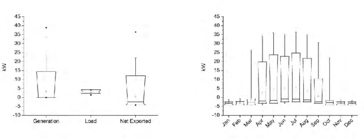
Chapter four presents the load match and grid interaction factors computed for all the case studies, with the exception of grid interaction indicators that could not be computed to the lack of the information of the design capacity connection. Results, benefits and drawbacks of the level of information given by each of the indexes have been discussed. Together with the numerical evaluation of the indicators, graphical representation of some indexes is proposed. The advantage of graphical representation is that it condenses a lot of information in a visual form. Graphical representation of load and supply cover factors (left and right, respectively in the next figure) in hourly values give a quite good picture of the correlation between on-site demand and supply of energy. It is possible to illustrate both the daily and seasonal effect, the production pattern of different renewable energy technologies, and applied operation/control strategies. 5 10 15 20 0 0.1 0.2 0.3 0.4 0.5 0.6 0.7 0.8 0.9 1 Hour of day M e a n o f L o a d c o v e r fa c to r 5 10 15 20 0.2 0.3 0.4 0.5 0.6 0.7 0.8 0.9 1 Hour of day M e a n o f Su p p ly c o v e r fa c to r Jan Apr Jul Oct
Page 7 of 102
A novel form of graphical representation using normalized load duration curve for net exported energy is proposed in this report. This graphical representation (see figure below) allows identifying the peak values of the net exported energy in a Net ZEB together with the profile of the grid interaction during the whole year knowing the percentage of time when the building is exporting energy. In the same graph, also the relation with the peak load, peak on-site generation and connection capacity are shown.
The report concludes that load and supply cover factor, together with the loss of load probability are enough indexes to describe the relationship with the on-site generation and the buildings load. Complementary to the annual values, hourly mean monthly values have been demonstrated very useful for describing both the seasonal and daily variations. In the case of grid interaction factors, the indexes which have been demonstrated more useful are the ones that can be extracted from the hourly values of the net exported energy. Generation Multiple is a useful index which relates the minimum and the maximum peak powers of the net exported energy, which gives additional information if statistical analysis of net exported energy is done and different percentiles are used to analyse the information. Additional indicators as capacity factor or dimensioning rate are indicators which allow to know at which extent a building is using the grid, however it needs knowing the design connection capacity between the building and the low (or medium) voltage grid. It has been demonstrated that in some cases the information of design connection capacity is hard to be known for designers of Net ZEBs, but it can be substituted by a reference or limit value alternatively. Dimensioning rate and Generation Multiple indexes have been demonstrated the usefulness to analyse cluster of Net ZEBs buildings with a limited information of the grip typologies.
Page 8 of 102
Although some aspects need to be developed in further research (as the extension to indexes to non-all electrical buildings) a selection of load match and grid indicators, together with graphical representation are proposed on the report based on their usefulness and their testing in both real monitored and simulated Net ZEBs.
Page 9 of 102
ACRONYMS
BAS Building Automation Systems
CHP Combined Heat and Power
DER Distributed Energy Resources
DG Distribute Generation
DHW Domestic Hot Water
DSO Distribution System Operators
EV Electrical Vehicle
GI Grid Indicators
GSHP Ground Source Heat Pump
LM Load Match
LMGI Load Match and Grid Interaction
MB Monitored Building
Net ZEB Net Zero Energy Buildings
NRA National Regulatory Authority
nZEB Nearly Zero Energy Buildings
PV Photovoltaic
RES Renewable Energy Source
SB Simulated Building
SH Space Heating
TSO Transmission System Operator
WP-SE Wood Pellet Stirling Engine
Page 10 of 102
1
INTRODUCTION
A thorough analysis of NZEBs must address the implications of two closely-related, highly dynamic phenomena: the continuous interplay between on-site generation and the building loads, and the resulting import/export interaction with the surrounding energy grid. The term load matching (LM) refers to the degree of agreement or disagreement of the on-site generation with the building load profiles; grid interaction (GI) refers to the energy exchange patterns between a building and the utility grid, and its impact on the overall load of the grid (Figure 1). Collectively, both issues are denominated LMGI.
Figure 1. Load matching (left) refers to the relationship between a buildings own generation and load. Grid interaction (right) alludes to the relationship between the energy exported/imported to the grid and the load conditions of the grid itself.
Net ZEBs have the dual role of being energy producers and consumers (“prosumers”). At all times, Net ZEBs must provide for the needs of their occupants by coordinating on-site generation with energy imports from the utility grid. Considering that Net ZEBs also export energy to the grid, their relationship with the utility grid is far more complex than that of conventional buildings, which may be seen as passive consumers.
Page 11 of 102
Time is essential in the analysis of LMGI issues. While the design of Net ZEBs has often focused on long-term energy balances, energy exchanges at smaller time scales (monthly, daily, hourly, sub-hourly) are critical. Within a building or within a utility network –as in any energy system– the limiting factor is the maximum power that may be delivered or received. Consequently, even if a building achieves a long-term energy balance between energy generated and consumed, smaller time scales must also be considered. For example, from the utility’s point of view, if a Net ZEB is a heavy consumer in winter it will appear to be quite similar to a conventional building, requiring the use of additional generation and transmission capacity. Keeping in mind that the driving concept behind Net ZEBs is the reduction of the environmental impact associated with buildings (e.g., oversized building service systems, intervention of polluting “peaking” power plants, construction of additional generation capacity, etc.), a comprehensive look on Net ZEBs must address LMGI issues, including quantitative indicators to characterize these issues. This report focuses on load management/grid interaction, in particular in the development, compilation and assessment of appropriate quantitative indicators.
For a long time the issue of the quality of exported energy and how it affects the energy system was out of the scope of Net ZEB concept. Buildings have been largely considered as passive consumers taking energy from the grid or other energy carriers (e.g., fuels) to supply their own needs. Whenever peak load reductions are achieved, it is often not the result of a deliberate effort, but the by-product of energy conservation measures (e.g., adding extra insulation results both in less energy use and smaller peaks). Annual energy use has traditionally been the gauge by which the energy performance of a building is described. Reducing peak loads adds an additional element of complexity to the task of maintaining a comfortable temperature while fulfilling all the other functions required in a building, such as communications, lighting, waste disposal, safety networks.
Another reason for the increasing importance of LMGI is the trend towards a more complex, flexible and dynamic energy system (Figure 2), with more renewable energy systems (both centralized and distributed), energy storage devices, electric vehicles, and smart metering. In this new state of affairs, there will be a continuous, bi-directional exchange of energy and information between Smart Buildings and the Smart Grid. Building automation systems (BAS) will do more than provide the building occupants with expected comfort services; they will also make optimal decisions about storing, exporting or importing energy resources depending on expected weather and occupancy patterns, and in response to signals from the grid.
Page 12 of 102
Figure 2. Links between the Smart Grid and Smart Buildings
In [1] the following potential target audiences for LMGI indicators have been identified: Building designers and owners
Community designers and urban planners Grid operators at a local distribution level Grid operators at a national or regional level
Policy makers and energy National Regulatory Authorities (NRAs).
Smart Grid Smart Buildings
Energy storage Electric vehicles Building automation system Occupants Building integrated renewables Energy + Information + 1359.1 Smart Meter Electricity + Heat Hydro Wind PV arrays Transmission and distribution networks Thermal plants
Page 13 of 102
2
TECHNICAL FRAMEWORK
In this section, a revision of the technical and economic conditions that can have an impact in the design and operation of Net ZEB is to be done. The review will be made from several perspectives. Different countries perspectives need to be analysed and compared.
2.1 NATIONAL / REGIONAL ENERGY SYSTEM
Operators of national energy grids (TSO – Transmission System Operator) are familiarized with economic dispatch and planning the operation of generation plants and transmission lines based on expected loads. Aggregated grid indicators at hourly or even higher resolution could help to manage national grids and to increase the penetration of renewables in the electric power system, especially if high daily peak/base load ratios occur.
As NZEB will be part of smarts grids, the question is whether NZEBs require a specific approach about integrating DER (Distributed Energy Resources) and power system balancing. As the penetration of NZEBs would probably be slow and limited in the near future (NZEB vs. nearly-ZEB) the question concerns more the impact of Net ZEBs in the mid and long term, as is the case of the forecasted role to play electrical vehicle (EV) for some TSO [18]. In any case, high resolution indicators linking Net ZEBs and national energy systems might be focused on strategic objectives (increasing the penetration of renewables or reducing external energy dependency) and they make sense if seasonal/daily variations need to be taken into account. These seasonal variations and features of the grid could vary from country to country and regionally within one country. Information or indicators for load matching and grid interaction can show whether added load and generation profiles will add to or reduce existing load variations, and thereby what to expect from Net ZEB expansion in the future. Figure 3 illustrates the difference of aggregated electrical generation profiles in Spain at winter and summer, showing the contribution of DER and wind generation to the total. Figure 4 illustrates the same concept for Sweden, where solar production is very low and the aggregated sum of renewable production is mainly due to wind. It can be appreciated that wind penetration in winter time in Spain can cover more than 30% of the electrical demand, especially at night. In the month of April 2013, power generation from renewable energy sources reached an all-time record representing 54% of production in Spain [27]. Also is clearly appreciated a pronounced seasonal variation in Sweden, and stronger daily fluctuations in load in Spain than in Sweden.
Page 14 of 102
Figure 3. Electrical generation in Spain in winter (February 2010 - left) and summer (July 2010 - right) representative weeks.
Figure 4. Electrical generation in Sweden in winter (January 2012 - left) and summer (July 2012 - right) representative weeks.
It should be noted, though, that at this level (i.e., national grid) the co-location of the building demand and the on-site generation, which is characteristic for Net ZEBs, is not as significant as at the local grid level. To balance the power system over a given area, it does not matter if the building loads and generation are located in exactly the same spot or geographically separated.
0 5 10 15 20 25 30 35 40 45 0 24 48 72 96 120 144 GW
Wind DER Total
0 5 10 15 20 25 30 35 40 45 0 24 48 72 96 120 144 168 GW
Wind DER Total
0 5 10 15 20 25 0 24 48 72 96 120 144 168 GW
Wind Solar Total
0 5 10 15 20 25 0 24 48 72 96 120 144 168 GW
Page 15 of 102
2.2 ELECTRICITY DISTRIBUTION GRIDS
This section makes a brief summary of the relevant concepts in power distribution and distributed generation necessary to understand the possible impact of Net ZEBs on distribution systems.
2.2.1 DISTRIBUTION GRID STRUCTURE, OPERATION AND PLANNING
The power system is constructed as a hierarchical arrangement, with a one-way flow of electrical power from a set of large-scale power plants to a large number of individual customers. Voltages are successively transformed to lower levels downstream in the grid. The distribution grid covers the lowest voltage levels and is usually divided into two parts, the middle-voltage (MV) grid, spanning 1-36 kV, and the low-voltage (LV) grid, with voltages below 1 kV [7]. Typically, in European grids, the LV voltage is 0.4 kV and the MV voltage is 10 kV. Distribution grids are normally constructed based on radial feeders, with the transformer substation at one end and the last customer at the other, and a number of customers connected along the way. The limiting factor for a distribution feeder is the voltage drop downstream along the feeder, which increases with the total load and the cable impedance.
Distribution system operators (DSOs) are required to keep network voltages within prescribed limits. According to the European standard EN 50160 [16], these are 90% and 110% of nominal voltage, but design limits are typically more narrow [8]. Primary transformer substations connecting the MV grid to the overlying high-voltage grid typically have automated voltage control through on-load tap changers to keep the voltage within bounds, but otherwise the distribution grid normally lacks surveillance and control. Secondary substations between MV and LV grids have manual tap-changer control with a constant turns ratio of the transformer that boosts the voltage to counteract the voltage drop in the MV grid.
When planning a distribution grid, the major factor is the expected peak load on the grid. This determines how large power flows the grid components have to handle. Once the expected load distribution is known, cables and transformers can be dimensioned to avoid overloading and to keep voltages within prescribed limits. It is important to note the effect that load coincidence has on the expected peak powers. For a set of buildings, their respective peak loads may be occurring around the same time but not exactly simultaneously, which effectively reduces the total peak load per customer. A commonly used method to size cables, depending on how many customers are connected, is the Velander method [7], which, in a simple mathematical formula, relates the expected peak power of a certain customer type to the total annual electricity consumption of a group of customers. An example is shown in Figure 5.
Page 16 of 102
This means, as an example, that each customer will contribute less to the capacity requirements of a main feeder connecting one hundred customers than to a single-customer connection downstream in the grid. As long as equipment connecting several customers is sized, load coincidence has to be taken into account. Thus, when grids for Net ZEBs are designed, or existing grids are adjusted for a conversion of buildings into Net ZEBs, similar rules of thumb will be useful, both for the load and generation parts.
Figure 5. Peak power contribution of customers in a distribution grid as predicted by the Velander method [7]. Evaluated for buildings with heat pumps and an annual electricity demand of 10 MWh.
2.2.2 HOSTING CAPACITY FOR DISTRIBUTED GENERATION
Net ZEBs are part of the more general concept of distributed energy resources (DER)1, which is
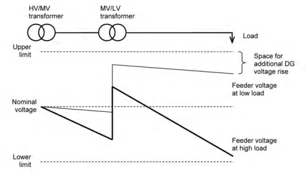
most straightforwardly defined as “electric power generation within distribution networks or on the customer side of the network” [9] Integration of DER into power systems is a large and active area of research that has given rise to a vast range of scientific publications. The most important findings are summarized in [8]. Distributed generation may be both beneficial and problematic for the operation of the distribution grid, depending on the penetration level. At modest penetration levels, DER provides benefits such as decreased losses in the local distribution grid and evened-out voltage profiles. For high penetration levels, injected DER power that is not consumed on-site may lead to substantial reverse power flows, increased local losses, overloading of grid components and voltage rise [10]. The impact of DER on grid voltages is outlined in Figure 6. Note that the grid voltage at any point in the grid is affected by the combined power flows to all customers.
Page 17 of 102
The hosting capacity concept has been introduced to describe and analyze the impact of distributed generation on a given distribution system design. In a very broad sense, the hosting capacity is the amount of distributed generation that can be connected to a distribution grid before the performance of the grid, measured by some suitable index, becomes unacceptable [8]. The concept is outlined in Figure 7. The performance index could be network losses, overloading of components, voltage levels or power quality measures. For distributed PV, which is the most common on-site power source for Net ZEBs, overloading and slow voltage variations are the most important factors [11][12]. Power quality issues, such as harmonic distortions, are normally resolved by PV inverters and fast irradiance fluctuations due to moving clouds over individual PV systems are still slow enough to be just on the verge of giving rise to flicker [8]. For spread-out PV systems, fast irradiance variability is reduced considerably [13] and does not have any impact on flicker-range voltage variations [8].
Figure 6. DG impact on voltages along a radial distribution feeder with 10 connected customers and a DG unit at the last node. At high load the voltage drop is reduced and at low load the voltage is raised above nominal. Reproduced from [10].
Page 18 of 102
Figure 7. Schematic outline of the hosting capacity concept. The hosting capacity is the penetration level of DER for which the chosen limit in performance is reached.
Two factors in particular may limit the hosting capacity for Net ZEBs with on-site PV generation within existing distribution grids. First, there is a considerable reduction of the expected peak power demand of an aggregate of buildings due to random coincidence of loads, as predicted by the Velander method, but this is not the case for the total PV generation, since at clear weather all systems will produce their maximum power at the same time. This means that while the marginal capacity that has to be added to supply an increasing number of loads decreases upstream in the grid, the capacity increase due to PV is directly proportional to the total PV capacity. Consequently, for a large number of customers, the load will be much more evenly distributed over time than the PV generation. If the total annual demand and on-site supply are equal, higher grid capacities are required to deal with the PV supply than the demand.
Second, tap-changers in secondary transformer substations are normally used to offset the nominal grid voltage to handle voltage drops. Since voltages in the grid are allowed to vary both above and below the nominal voltage, this allows a larger span of the voltage variations. At low load, connections upstream in the grid are maximally above nominal voltage, and at high load, connections downstream are maximally below nominal, as indicated by Figure 8. The figure also shows how this may limit the amount of PV generation possible to connect. Since the highest peak powers are injected at times of low overall load on the grid, the tap-changer offset could severely limit the allowed voltage variations due to on-site PV.
Page 19 of 102
Figure 8. Schematic outline of how tap-changer voltage control limits the hosting capacity for DG.
The hosting capacity for distributed PV depends on the structure, strength, load distribution and operation and control of the individual grid. There are several previous studies taking the above factors into account (see e.g. [10][14]), and all come to varying conclusions about hosting capacities and allowed penetration levels. In general, though, city grids are more robust than suburban or rural grids. For example, in a Swedish simulation study, it was found that representative rural and suburban grids could allow a 60% PV penetration of the annual demand before the allowed voltage was exceeded, while a representative city grid would allow PV penetrations three times higher than the annual demand [11].
The business-as-usual option to increase the hosting capacity of a distribution grid is grid reinforcement, i.e. using cables with lower resistance and reactance. However, these investments could prove costly for the DSO, which is why other options to increase the hosting capacity are currently studied in international research, including altered tap-changer control, reactive power provision by PV inverters, PV power curtailment and increased PV self-consumption by demand response measures or local storage [14]. Studies for Sweden have shown that the former three methods can have a considerable impact on the highest peak injections [11], while the effect of demand-response measures, at least through automated appliance scheduling, is limited [15].
Page 20 of 102
2.2.3 RELEVANT HIGH-RESOLUTION INDICATORS FOR NET ZERO ENERGY BUILDINGS
The above discussion highlights two things. First, planning for urban environments with Net ZEBs will require distribution grid planners to take both building loads and on-site generation into account; so that the grid can handle both the highest peak demands and the highest injected peak powers. Second, the Net ZEB design, with a fixed relation between the on-site generation and the building demand, provides planners with limits to the powers that must be handled by the distribution grid, i.e. if the power demand of the building is known, so is the amount of power generated on-site. For a given Net ZEB, or a set of Net ZEBs, it should be possible to find a relation between the expected peak demand and the expected peak power generation, which is the information required.
The central physical parameter in the distribution grid interaction is the magnitude of the power (active and reactive) injected or consumed by a group of customers. This will determine the power flow through the grid components and, consequently, currents and voltage levels. Variability is not important per se, but variability and coincidence determine which power levels occur and how often. Relevant grid interaction indicators for distribution grid planning should show, or be based on:
- The relation between the expected net peak power demand and the expected net peak power generation for an arbitrary set of typical buildings, both of these in relation to the total annual consumption/generation. With this information, it is possible to choose grid components that can handle all power imports and exports from any group of customers of varying size. Ideally, these should be in the form of rules-of-thumb or formulae similar to the Velander method. Note that load and generation coincidence are crucial for grid design and operation, hence an indicator for the individual building is not sufficient as long as components interconnecting several consumers are considered (which is mostly the case).
Page 21 of 102
- The distribution of power exports and imports above a certain threshold value over a certain period of time (typically a year). This shows how often peak powers of a certain magnitude occur. It may be relevant, for example, if curtailment of injected power is required. Instead of dimensioning grids to handle all power exports and imports from buildings, requirements may be put on distributed generators to provide reactive power as grid support, or curtailment of the power output. There could also be requirements on generators to participate in frequency control and time-differentiated tariffs or other incentives could be given to the customers to alter their demand profiles. Quantifying the occurrence of peak powers of a certain magnitude indicates how often problematic levels are achieved with a certain building design and operation.
2.2.4 REQUIRED ELECTRICAL PEAK LOADS FOR LOW-VOLTAGE SUPPLY
As it has been highlighted before the expected peak power demand of one building or cluster of buildings is key information to generate relevant indicators or establish threshold values that indicators can refer to. As example, Table 1, shows the minimum electrical supply requirements in Spain [17].
Table 1.Minimum requirements for electrical supply in buildings in Spain
Type Minimum Power
Residential, Individual
basic level 5 750 W @ 230 V
Residential, Individual
high level2 9 200 W @ 230 V
Residential, Collective Simultaneity factor applied to sum of requirements for individual dwellings. (Plus ancilliary spaces) Office buildings 100 W/m2 or 3 450 W/space @ 230 V
Simultaneity factor = 1
Page 22 of 102
2.3 BUILDING DESIGNERS / OWNERS PERSPECTIVE
When evaluating load match and grid interaction, reliable or probable forecasts of the building energy consumption and production on hourly or sub-hourly scale are important. A significant challenge regarding this aspect is the lack of methodologies and standardised tools to make hourly or sub-hourly forecasts based on factors such as the number of occupants or orientation of the PV panels. The existing design approach and building certification programmes are mostly focused on the implementation of energy efficiency measures and hence reduction of energy use [24], and do not usually contain hourly load/generation profiles or, as maximum, contain average profiles.
Economy is often the driving force of the building owners. Thus, when determining or evaluating the building’s energy export and import, the economic benefit is determined by the price difference between energy sold to the utility company and energy bought from the utility. These aspects may vary from country to country – and even within each country. As example, in Germany due to policy incentives, consumers receive less for electricity sold to the utility than what they pay for buying electricity from the utility. This makes it beneficial to maximise self-consumption, i.e. minimising export of electricity to the grid. In such a case, households would benefit from having PVs orientated east-west as they will produce electricity in the morning and in the afternoon, following the load profile. In the case of an office building, the PVs might be orientated south as peak load occurs during midday. If an opposite price regime occurs, for example by feed-in tariffs, that makes the price of electricity sold to the grid higher than the price of electricity bought, the orientation of the PV panels should give the maximum production regardless of the shape of the load profile, as the matching is not an important issue. If the spot price of electricity is the only incentive (no subsidies or other policy incentives), the owner may shift load according to the fluctuating electricity price, hour by hour. In both the first and the last case, more flexible demand will make the building more capable of profiting from its onsite production. In these cases, building designers or owners should arrange for making the load and grid interaction as flexible as possible.
Page 23 of 102
3
LMGI INDICATORS
3.1 INTRODUCTION
This section presents quantitative and relevant indicators that can be used to describe Load Matching and Grid Interaction (LMGI) conditions in net-zero or near net-zero energy buildings (Net ZEBs). Load Matching refers to how the local energy generation compares with the building load. Grid Interaction refers to the energy exchange between the building and an energy infrastructure, typically, the power grid. These are independent, but intimately related issues. The main distinction made here is that load matching indicators measure the degree of overlap between generation and load profiles (e.g. the percentage of load covered by on-site generation over a period of time) whereas grid interaction indicators take aspects of the unmatched parts of generation or load profiles into account (e.g. peak powers delivered to the electricity distribution grid).
A comprehensive revision of LMGI indicators are given in [1] together with some proposals for alternative indicators. These indicators have been used to evaluate Net ZEB test cases [1][6][21], while some other indicators are also proposed in the literature [5][20][23]. The indicators selected and described in this section will be evaluated in the following sections through case studies.
Page 24 of 102
3.2 TERMINOLOGY
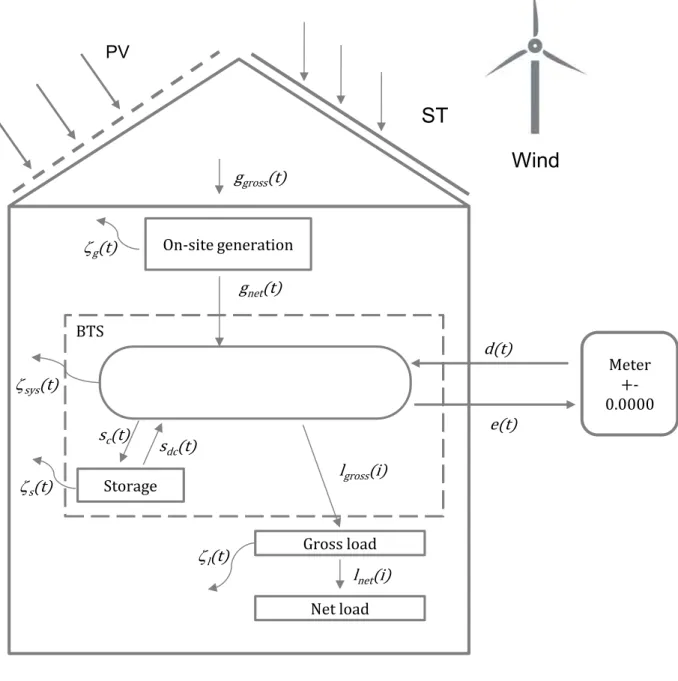
The sketch depicted in Figure 9 provides an overview of relevant terminology addressing the energy use in buildings and the connection between buildings and the power grid.
Figure 9. Schematic view of the energy flows in a Net ZEB
Load (L
PV Meter +-0.0000 Storage d(t) Gross load e(t) gnet(t) lgross(i) sc(t) sdc(t) On-site generation zg(t) ggross(t) zs(t) BTS zsys(t) Net load lnet(i) zl(t)ST
Wind
Page 25 of 102 Nomenclature
t time
e, E exported energy d, D delivered energy ne net exported energy g, G on-site generation
gnet net on-site generation
ggross gross on-site generation ̅ average on-site generation sc charging storage energy
sdc discharging storage energy
S storage energy balance Us Internal storage energy
T evaluation period
start of the evaluation period
end of the evaluation period w weighting factor
l, L load
lnet net load
lgross gross load ̅ average load energy losses
generation energy losses storage energy losses
Building technical systems energy losses (excluding storage)
Load energy losses (e.g.: distribution losses) BTS Building Technical Systems
Edes Designed/required connection capacity
Subindex
i energy carrier
d delivered
e exported
Page 26 of 102
The core principle for Net ZEBs is the balance between the weighted demand and weighted supply [2], which is described in Eq. 1, based on delivered and exported energy quantities, where i stands for energy carrier.
∑ ∫ ( ) ( ) ∑ ∫ ( ) ( )
Eq. 1
A general energy balance in the building is represented with Eq. 2
( ) ( ) ( ) ( ) ( ) ( ) ( ) Eq. 2 where ( ) ( ) ( ) Eq. 3 ( ) ( ) ( ) Eq. 4 ( ) ( ) ( ) ( ) Eq. 5 ( ) ( ) ( ) Eq. 6
If we integrate over time between 1 and 2 (the evaluation period), then we have
∫ ( ) ∫ ( ) ∫ ( ) ∫ ( ) ∫ ( ) ∫ ( )
Eq. 7
∫ ( ) ∫ ( ) ∫ ( ) ∫ ( ) ∫ ( ) ∫ ( )
Page 27 of 102
If we consider that over the evaluation period, , then:
∫ ( ) ∫ ( ) ∫ ( ) ∫ ( ) ∫ ( )
Eq. 9
Net exported energy is defined as:
( ) ( ) ( ) Eq. 10
A graphical presentation using Sankey diagrams could help to understand the energy flows and the energy balance. An example for a Norway case is presented here.
Figure 10. Schematic illustration in form of a Sankey Diagram for a Net ZEB [21]
Gr o ss e n e rg y d e m an d N e t e n e rg y d e m an d D e liv e re d e n e rg y Building’s energy system Passive gains Internal heat gains On-site renewable energy production Heat from surroundings Losses Pr im ar y e n e rg y d e m an d Extraction Production Storage Transport …
Technical regulations Energy label (Norway) EPBD
Ref: Rasmus Z. Høseggen, Ph.D. Associate Professor II, NTNU and Senior advicer, Evotek
GHG emissions
Lo
ss
Page 28 of 102
3.3 LOAD MATCH INDICATORS
Load match indexes intend to describe the degree of the utilisation of on-site energy generation related to the local energy demand.
3.3.1 LOAD MATCH INDEX
The first proposed index was the load match index [22], defined as the average value over an evaluation period of how the on-site generation covers the energy load. The load match index intends to describe the matching degree between on-site energy generation and the building load. As higher the index is, better the coincidence between the load and the onsite generation. The formulas describing the load match index vary from very general ones [2,22], which do not specify if storage and losses of energy are included, to very clear definitions [1, 6].
∑ [ ( ) ( )] Eq. 11 [2] [ ( ) ( ) ( ) ( ) ] ̅̅̅̅̅̅̅̅̅̅̅̅̅̅̅̅̅̅̅̅̅̅̅̅̅̅̅̅̅̅̅̅̅̅̅ ∑ [ ( ) ( ) ( ) ( ) ] Eq. 12 [1]
where N is the number of samples in the evaluation period, from 1 to 2. In case that hourly resolution data are used and the evaluation period is a complete year, the number of samples is 8760.
In this study the most detailed formula is used, which indicates that storage as well as losses of energy should be included in the load match index calculation.
3.3.2 LOAD COVER FACTOR AND SUPPLY COVER FACTOR
Load cover factor is also described in [1] and represents the percentage of the electrical demand covered by on-site electricity generation and is defined as
∫ [ ( ) ( ) ( ) ( )] ∫ ( )
Page 29 of 102
Then a complementary index, the supply cover factor, can be defined representing the percentage of the on-site generation that is used by the building. Mathematically, it could be defined as:
∫ [ ( ) ( ) ( ) ( )] ∫ [ ( ) ( ) ( )]
Eq. 14
or as in equation Eq. 15, if storage and system losses are not subtracted from the on-site generated energy.
∫ [ ( ) ( ) ( ) ( )] ∫ ( )
Eq. 15
In [20], two factors are computed. The REF – Renewable Energy Factor (very similar to the load cover factor) and the REM – Renewable Energy Matching (similar to the supply cover factor).
∫ [ ( ) ( ) ( )] ∫ ( ) Eq. 16 ∫ [ ( ) ( ) ( )] ∫ ( ) Eq. 17
In [5], the demand cover factor (or self-generation) for all-electric buildings are defined as:
∫ [ ]
∫
Page 30 of 102
Where PS is the local power supply and PD the local PV power demand. The term [ ]
represents the part of the power demand instantaneously covered by the local PV power supply or the part of the power supply covered by the power demand. Also, in [5], the supply cover factor (or self-consumption) for all-electric buildings is defined as:
∫ [ ] ∫
Eq. 19
Table 2 shows the equivalence between the load and supply cover factors and other nomenclatures for the load match indexes in the literature.
Table 2. Equivalence of cover factors in the literature
Load Cover factor
Renewable Energy Factor
REF
Demand cover factor (self-generation)
Supply cover factor
Renewable Energy Matching
REM
Supply cover factor (self-consumption)
[1] [20] [5] references Literature
A conceptual item related with the computation of the cover factors (and thus related with the computation of share of renewables in a building) is the treatment of losses. In the nomenclature, we have distinguished between:
Storage losses
Building technical systems losses (excluding, storage losses) Load losses (for example, distribution losses)
Page 31 of 102
In Eq. 13, Eq. 14 and Eq. 15, the sum of the storage losses and the variation of internal energy in the storage sub-system (S(t)) and the system losses ( ( )) are subtracted from the on-site generation. In [1], system losses are subtracted from on-site generation In [21], storage losses and distribution losses are distinguished. Although is not completely clear, it seems that only storage losses (difference between charging and discharging storage system) is subtracted from on-site generation to compute the load match factor In [6], same computation as in [1] is used.
In [20], two factors are computed. The REF – Renewable Energy Factor (very similar to the load cover factor) and the REM – Renewable Energy Matching (similar to the supply cover factor). Although losses are considered in the balance, they are not subtracted to the on-site generation to compute REF or added to the load to compute REM. ES(t) and HS(t) in [20] represents storage balance in the battery (ES) and in the solar tank of the system (HS) (then charging minus discharging). In [5], where Eq. 18 and Eq. 19 are defined, no electrical storage system is considered in the model and a water storage tank is considered as part of the thermal building system model. The model only includes BIPV as renewable generation system and is connected to the electrical grid.
3.3.3 DIFFERENCE BETWEEN LOAD COVER FACTOR AND LOAD MATCH INDEX
The two factors can be defined either in the continuous domain, i.e. using integral notation (∫), or in the discrete domain, i.e. using the summation notation (∑). In literature the load cover factor, is presented with the integral notation [1][5]while the load match factor, , is presented with the summation notation [2]. For the sake of comparability they are both presented here in the integral notation, given that the considerations developed below would hold true also for the summation notation.
The two factors are meant to express the same thing, i.e. the share of the load (energy demand) that is covered by the on-site generation (energy supply) for a specific energy carrier. Nevertheless the two factors are not identical, since their mathematical definition is different, as shown in the following table. The factors are first defined as found in literature, but using integral notation for both of them and using the same nomenclature. Thereafter the two factors are further manipulated in order to write them in a comparable fashion and highlight the difference.
Page 32 of 102
load cover factor, load match index,
∫ [ ( ) ( )] ∫ ( ) ∫ [ ( ) ( )] ̅∫ [ ( ) ( )] ∫ ̅ [ ( ) ( )] ∫ ( ( ) ( )) ∫ ( ( ) ( ) ( ) ( )) ∫ ( ) [ ( ) ( )]
It should be noticed the difference inside the integral sign: while the load cover factor has
̅⁄, which is a constant quantity, the load match factor has ⁄ ( ), which is a quantity varying with time. This causes a numerical difference between the two indicators, which in most cases may be expected to be small but is nevertheless a difference.
It may be argued that has a somehow more intuitive definition, being the ratio between two quantities. Furthermore, a closer look shows that actually beholds a mathematical property that does not have, as shown below. With starting point from the last form of equation form the previous table it can be seen that:
̅ ∫ [ ( ) ( )]
̅ ̅
Eq. 20
if we define ̅ = average , where:
Page 33 of 102
Therefore represents the arithmetic average between two quantities. The same cannot be said for since it contains inside the integral the time dependent term ⁄ ( ). This gives to the load cover factor a somewhat more elegant mathematical formulation than the load match factor .
Finally, as discussed in [5] and in the previous sub-chapter 3.3.2, the load cover factor may be used in combination with the supply cover factor , which is defined in a symmetrical way as the share of the on-site generation (energy supply) that is covered by the load (energy demand). The two cover factors and would have the same numerical value when the balance for the energy carrier is exactly zero in the observed period, while it would differ for nearly zero or plus balances. An attempt to create a similar symmetrical factor of would fail to reproduce the same behaviour – i.e. having the same numerical value when balance is exactly zero – for the reasons explained above.
In conclusions, although the two indicators appear similar, the load cover factor is to be preferred for the reasons explained here and it is proposed to be used instead of the load match index. The rest of this report will therefore address the load cover factor and disregard the load match index .
3.3.4 LOSS OF LOAD PROBABILITY
The loss of load probability (LOLP) can be defined as the percentage of time that the local generation does not cover the building demand, and thus how often energy must be supplied by the grid. This index could be useful to evaluate different load control strategies in a building.
∫
( ) ( ( ) ( ) ( ))
Eq. 21
An equivalent method to define this indicator based on exported/delivered energy is:
∫
( )
Page 34 of 102
3.4 GRID INTERACTION FACTORS
Grid interaction factors can be computed using actual power values or can be presented using normalized values. As the objective of computing grid interaction factor is to measure how the utilisation of the grid connection is in relation to the building or a cluster of buildings, we propose to use the design connection capacity as normalizing quantity.
The nominal grid connection capacity is denoted by Edes 3.4.1 PEAK POWER GENERATION/EXPORTED
This indicator represents the normalized peak value of the on-site generation or exported energy. ̅̅̅̅̅̅ [ ( )] Eq. 23 ̅ [ ( )] Eq. 24
3.4.2 PEAK POWER LOAD/DELIVERED
The normalized peak power of the load or delivered energy is represented by the following equations. ̅̅̅̅̅̅ [ ( )] Eq. 25 ̅ [ ( )] Eq. 26 3.4.3 GENERATION MULTILPLE
The generation multiple relates the size of the generation system with the design capacity load. It is expressed as the ratio between generation/load peak powers or exported/delivered peak powers. ( ⁄ ) [ ( )] [ ( )] Eq. 27 ( ⁄ ) [ ( )] [ ( )] Eq. 28
Page 35 of 102
3.4.4 DESIGN RANGE
The design range is defined as the amplitude between the generation/load or the exported/delivered energy values.
Eq. 29
3.4.5 NET EXPORTED VALUES AND RANGES
Defining the normalized variable for the net exported energy as:
(
̅̅̅̅̅̅) ( )
Eq. 30
The maximum and minimum peak power can be defined as:
̅̅̅̅̅̅̅̅ [ ( ̅̅̅̅̅̅)] Eq. 31
̅̅̅̅̅̅̅̅ [ ( ̅̅̅̅̅̅)] Eq. 32
Having the possibility to statistically analyse net export values, the following values can be computed | | | |; | ( ) | | ( ) |; | ( )| ( ) | | ; | ( ) | | ( ) | 3.4.6 CAPACITY FACTOR
The capacity factor shows the total energy exchange with the grid divided by the exchange that would have occurred at nominal connection capacity, i.e., a measure of the utilisation of the grid connection.
∫ | ( )|
Page 36 of 102
We discard to use the alternative capacity factor defined in [1] which indicates the path of the energy exchange with the grid. Although, it makes sense for instantaneous values or short periods of time, the annual value for a Net ZEB with the definition in [1] will be always equal to 0.
3.4.7 DIMESIONING RATE
The dimensioning rate is the maximum absolute value of the net exported energy and thus it will coincide with ̅̅̅̅̅̅̅̅ or ̅̅̅̅̅̅̅̅
[| ( )|]
Eq. 34
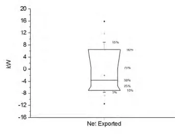
The sketch in Figure 11 intends to show the main values expressed in the equations above.
Figure 11.Example of load duration curve for normalized net exported electricity. Also the values of ̅̅̅̅̅̅
and ̅̅̅̅̅ are shown in the graph (horizontal red and green dashed lines) together with the normalized
value of Edes (+1 and -1).
3.4.8 CONNECTION CAPACITY CREDIT
The connection capacity credit, or power reduction potential originally defined in [23], can be defined as the percentage of grid connection capacity that could be saved compared to a reference case. It can be reformulated as
Page 37 of 102
Positive values of the index indicates a saving potential with respect to the reference case, and negative values means there is a need to increase the grid connection.
On the other hand, taking the connection capacity as reference, it will be possible to identify the power reduction potential
Eq. 36
On the contrary, if the reference case is the a building with no on-site generation, the following equation can be defined, to characterize the power reduction potential
( ) ̅̅̅̅̅̅ Eq. 37
3.4.9 PEAKS ABOVE CERTAIN LIMIT
The peaks above certain limit value indicate the part of analysed period that net export energy exceeds a certain barrier. The generic formulation is:
∫ | ( )|
Eq. 38
Considering that the grid connection capacity should never be exceeded, in case that the aim is to limit the grid connection capacity the limit value should be the capacity that is aimed at. Other suggested value could be a certain value which is a turning point for which contracting or grid connection rules are to be fulfilled in relation to connection to the local grid distribution.
3.5 OTHERS GRID INTERACTION INDICATORS 3.5.1 NO GRID INTERATION PROBABILITY
This index means the probability that the building is acting autonomously of the grid. In that case, the entire load is covered by the direct use of renewable energy or by the stored energy
∫ | ( )̅̅̅̅̅̅̅̅|
Page 38 of 102
3.5.2 GRID INTERACTON INDEX
The grid interaction index indicates the variability of the exchanged energy between the building and the grid within a year normalized on the maximum absolute value.
( (| ( )|) ( ) ) Eq. 40
3.5.3 GRID CITIZENSHIP TOOL
The aim of this tool is to qualitatively estimate the way that an interconnected component e.g. an energy producing building or a microgrid of such buildings, interacts with a greater power system, e.g. low-voltage power grid. It consists of the following factors: component ratio (CR) – describes the proportion between on-site generation and load; storage ratio (SR) – gives a qualitative indication of how well on-site generation is supported by on-site storage; intermittency ratio (IR) – indicates how reliable the component is at supplying energy. CR and SR factors are between -1 and 1, and IR varies from 0 to 1.
Eq. 41 Eq. 42 Eq. 43
Page 39 of 102
3.5.4 EQUIVALENT HOURS OF STORAGE
The equivalent hours of storage corresponds to the storage capacity expressed in hours. The physical capacity is the number of hours of storage multiplied by the power design load. This index should be explored as potential indicator of flexibility in buildings with storage system.
Page 40 of 102
4
CASE STUDIES
4.1 MONITORED BUILDINGS
The monitored data are available for six buildings, which represent different building topologies and renewable energy technologies. Table 3 gives an overview of seven case studies which are identified using the notation MB, for monitored buildings. Not all six buildings are fulfilling the zero energy standards. This is the case of MB5: two set of data are available for this multifamily house in Italy (2009 and 2011) being the data of year 2011 closer than the zero balance due to a reduction of loads and greater energy generated from the PV system. MB1 which is a house in Denmark and MB6 which is a refurbished building in Germany where a CHP system was installed are nearly ZEB.
Table 3.Overwiew of the case studies: Monitored Buildings
Case
study Country Building type Technologies infrastructure Energy Resolution Time
MB1 Denmark Single family house
Photovoltaic / Heat pump
+ Solar Thermal Electricity grid 1 hour MB2 Denmark Single family
house
Photovoltaic / Heat pump
+ Solar Thermal Electricity grid 1 hour MB3 Denmark Single family
house
Photovoltaic + Solar
Thermal / Heat pump Electricity grid 12 min MB4 Singapore Office Photovoltaic / Electric driven chillers Electricity grid 1 hour (year) MB5 Italy Multi- family house
Photovoltaic + Solar Thermal /Heat pump /
Cooking system with methane
Electricity grid &
methane 1 hour
MB6 Germany Multi- family house
Gas driven CHP, additional condensing
boiler, water storage, smart control
Electricity & gas
grid 5 min MB7 Sweden Single family
house
Photovoltaic + Solar
Page 41 of 102
Figure 13. ZEB status exported v. delivered for the monitored buildings. Figures are in kW·h/m2 (Primary
Energy) 0 40 80 120 160 200 240 0 40 80 120 160 200 240 Ex p o rte d [ kWh /m² ] Delivered [kWh/m²] MB1 MB2 MB3 MB4 MB5_2009 MB5_2011 MB6 MB7
Page 42 of 102
4.1.1 MB1 AND MB2-FLAMINGO HOUSE -DENMARK
The Flamingo house is a single family house in Denmark, with a gross floor area of 166 m² living space. The house was built in 2008 and is occupied by a family: two adults and two children.
The annual space heating demand is calculated to be 18 kWh/m². The energy system is composed by 16 m2 of PV panels (2 kWp), 8 m² of thermal solar collectors for domestic hot water and space heating and a 5 kW ground coupled heat pump for both domestic hot water and space heating. More details may be found on: www.flamingohuset.dk (unfortunately only in Danish).
Measurements are available for more than one year since February 2009, in 1-hour resolution. For the analysis in that report data corresponding to the year 2012 has been selected (MB1). The Flamingo house is not a Net ZEB. Then, a variation of the MB1 case has been generated artificially with the hypothesis of increasing the PV capacity by a factor of 4.5, which is identified as the MB2 case study.
Table 4.Features of the MB1 and MB2 case studies. The Flamingo house
Characteristic Value Installed PV capacity – MB1 2.0 kWp Installed PV capacity – MB2 10.0 kWp
Installed PV area – MB1 16 m2
Solar thermal area 8 m2
Building area 166 m2
Design connection capacity 10 kW3
Thermal storage
capacity/volume 300 litres Electrical storage capacity -
Page 43 of 102
4.1.2 MB3-ENERGY FLEX HOUSE -DENMARK
EnergyFlexHouse® consists of two, two-storied, single-family houses in Denmark, with a total heated gross area of 216 m² each. The two buildings are in principle identical, but while the one building acts as a technical laboratory (Energy-FlexLab), the other is occupied by typical families who test the energy services (EnergyFlexFamily). The houses are built so they are better than the Low E class 1 defined in the former Danish Building Code from 2008. The annual energy demand for space heating, ventilation, DHW and building-related electricity (not including energy for the household) amounts to less than 30 kWh/m². With the PV production, EnergyFlexFamily is energy neutral over the year including the demand for electricity of the household and an electric vehicle. The heating system consists of two heat pumps and a solar heating system. One of the heat pumps produces space heating via the floor heating system. The other heat pump is located in series with the passive heat exchanger of the ventilation system. This heat pump both preheats fresh air and DHW. The solar heating system preheats primarily DHW but may also deliver space heating. The efficiency of the passive heat exchanger is around 85%.
The layout of the two houses is similar to the layout of many Danish single-family houses, although reversed concerning the use of the two floors. The buildings were put into operation during the autumn of 2009. Analyzed data corresponds to year 2010 which has been recorded with a 12 minutes resolution and do not include EV consumption.
Table 5.Features of the MB3 case study. The EnergyFlex house.
Characteristic Value Installed PV capacity 10.6 kWp
Installed PV area 60 m2
Solar thermal area 4.8 m2
Building area 216 m2
Design connection capacity 25.2 kW4
Thermal storage
capacity/volume 180 litres Electrical storage capacity -
Page 44 of 102
4.1.3 MB4- ZEB@BCAACADEMY -SINGAPORE.
ZEB @ BCA Academy is a non-residential-Educational building, with PV generation, located in Singapore. This building is operating since 2009, with a 4.500 m2 of net floor area and 2.018 m2 of conditioning area. The ZEB project is intended as a functioning demonstration in the efficient use of energy in a building through both passive and active means for which a section of the existing BCA Academy has been converted for this purpose. Glazing, lightweight wall systems, shading devices, light shelves and green walls are incorporated into the west facade. Some rooms at the ground level have ducting of natural light for illumination. Light tubes are also installed to direct light into the interior of an office environment. The roofs are covered with solar PV panels to generate sufficient electrical energy to be self-sustaining, and certain part of the roof incorporates a ventilation stack to test the effect of convection air movement within a naturally ventilated environment.
Table 6.Features of the MB4 case study – ZEB @ BCA Singapore
Characteristic Value Installed PV capacity 190 kWp
Installed PV area 1 540 m2
Building area 4500 m2
Design connection capacity 200 kW Electrical storage capacity -
Page 45 of 102
4.1.4 MB5-LEAF HOUSE -ITALY
Leaf House is a technologically innovative muti-family house: its characteristics of cheapness, simplicity, efficiency and silence combine and integrate to create a house made for the environment. Leaf House is a clean energy laboratory, a place to be studied and visited, awakening and educating people to future. Leaf House is an example of saving and respect; it is a house composed of six flats, a real house where real people live. The average electric consumption per family in Ancona area corresponds to about 2100 kWh/year. With all the precautions used in the Leaf House, the electric consumption should not exceed the 1.500 kWh/year. All consumptions are monitored and just after the first year of use it will be possible to have more reliable data. The house is provided with a geothermal heat pump and thetechnical systems are completed by a solar thermal collectors field and a photovolatic system. The electric consumptions including the air-conditioning and the heating system ones are covered by the photovoltaic plant integrated in the building cover. Real monitored data are available with 1 hour time resolution. Two set of data are analysed in this report corresponding to year 2009 and 2011.
Table 7.Features of the MB5 case study – The Leaf house
Characteristic Value Installed PV capacity 20.0 kWp
Installed PV area 150 m2
Solar thermal area 19 m2 Building area 480 m2 Design connection capacity 50 kW
Thermal storage
capacity/volume 1000 litres Electrical Storage capacity -
Page 46 of 102
4.1.5 MB6–CHPWUPPERTAL-GERMANY
A combined heat and power unit (CHP) with smart control was integrated in the heat supply of a typical multifamily building in Wuppertal, dated from early 1900 [31]. Buildings of this type are characteristic for many cities in Germany and form the appearance of old town quarters with complete perimeter block developments. Due to heritage for the historical facades, thermal insulation measures are limited and expensive. The original heat supply was a central natural gas boiler for space heating by radiators combined with electric heaters for DHW in the individual apartments. The measured gas consumptions achieved 145 kWh/m²·y before the modification of the heating system. With a research project supported by the foundation “Zukunft NRW” the building was equipped with a central CHP unit using natural gas and assisted by a condensing boiler for peak heat loads. The DHW water supply was combined with the central heating system to generate an additional, all year round heat load. To allow flexibility in operation times and cycles of the CHP a 2 m³ water tank acts as thermal buffer together with the very high thermal mass of the building structure. The experimental control system is based on a cost optimization function and a prediction algorithm for the thermal and electric load of the building. In practice the CHP unit was very flexible operated with respect to the power needs without neglecting coverage of the heat demand. Almost no use of the gas boiler was recorded (only Jan/Feb). The total gas consumption in 2011 was measured to 171 kWh/m²/y combined with 61 kWh/m² of electricity generation, of which 28 kWh/m²/y were supplied to the grid and the other 33 consumed in the households.
Table 8.Features of the MB6 case study - CHP Wuppertal - Germany case study
Characteristic Value
Installed CHP power 5.5 kW Installed CHP heat 14.8 kWt
Installed gas burner capacity 14.0 kWt
Building area (heated) 465 m2
Number of occupants 12 persons Design connection capacity 80 kW5
Thermal storage capacity/volume 2000 litres + 300 litres (DHW) Electrical storage capacity -
5 80 kW is the reference value for the case of electric supply for DHW; 40 kW in case that DHW is supplied by othar energy carriers / systems (CHP,