A rulebased classifier with accurate and
fast rule term induction for continuous
attributes
Conference or Workshop Item
Accepted Version
Almutairi, M., Stahl, F. and Bramer, M. (2019) A rulebased
classifier with accurate and fast rule term induction for
continuous attributes. In: 17th International Conference on
Machine Learning and Applications, 17th to 20th of December
2018, Orlando, Florida, pp. 413420. Available at
http://centaur.reading.ac.uk/80938/
It is advisable to refer to the publisher’s version if you intend to cite from the
work. See
Guidance on citing
.
Published version at: https://ieeexplore.ieee.org/document/8614093All outputs in CentAUR are protected by Intellectual Property Rights law,
including copyright law. Copyright and IPR is retained by the creators or other
copyright holders. Terms and conditions for use of this material are defined in
the
End User Agreement
.
www.reading.ac.uk/centaur
CentAUR
Central Archive at the University of Reading
Reading’s research outputs online
A Rule-Based Classifier with Accurate and Fast
Rule Term Induction for Continuous Attributes
1
stManal Almutairi, Frederic Stahl
Department of Computer Science University of Reading Reading, United Kingdom Email: [email protected]
2
ndMax Bramer
School of Computing University of Portsmouth Portsmouth, United Kingdom
Abstract—Rule-based classifiers are considered more expres-sive, human readable and less prone to over-fitting compared with decision trees, especially when there is noise in the data. Fur-thermore, rule-based classifiers do not suffer from the replicated subtree problem as classifiers induced by top down induction of decision trees (also known as ‘Divide and Conquer’). This research explores some recent developments of a family of rule-based classifiers, the Prism family and more particular G-Prism-FB and G-Prism-DB algorithms, in terms of local discretisation methods used to induce rule terms for continuous data. The paper then proposes a new algorithm of the Prism family based on a combination of Gauss Probability Density Distribution (GPDD), InterQuartile Range (IQR) and data transformation methods. This new rule-based algorithm, termed G-Rules-IQR, is evaluated empirically and outperforms other members of the Prism family in execution time, accuracy and tentative accuracy.
Index Terms—Modular Classification Rule Induction, Dynamic Rule Term Boundaries, Interquartile Range Rule Term Bound-aries
I. INTRODUCTION
Decision tree based classifiers are popular for their accuracy and their simplicity to be converted into a set of rules by transforming each leaf of the tree into a rule. However, when dealing with large datasets, decision trees tend to become very large, complex, and difficult to understand. Consequently, the rules constructed through ‘Divide and Conquer’ strategy and extracted from the resulting decision tree inherit the tree’s complexity and thus may have unnecessary repeated tests which can lead to redundant rulesets [1], [2]. In this context, research has been carried out aiming to overcome or reduce these problems and to produce a simple reliable ruleset using pruning methods. Among others, C4.5rules [3], [4] and CART [2] are examples of such algorithms. Nevertheless, [5]–[7] argue that there is no single study which adequately achieves this goal. Cendrowska [6] recognised the disadvantages of gen-erating a ruleset in the form of a decision tree and criticises this method as a main source of over-fitting due to the replicated sub-tree problem that occurs when rules with no common attributes are forced to fit in a tree structure. Therefore, she developed Prism as an alternative expressive rule induction algorithm that follows a different rule induction approach called ‘Separate and Conquer’. This approach can extract if-then rulesets directly from training data. Several experiments
conducted in [8] indicate that Prism is an ideal representative for ‘Separate and Conquer’ algorithms, it cannot only perform at the same level of accuracy as tree based methods but also in most cases outperforms them in terms of classification accu-racy and computational efficiency, especially if there is noise in the data. RIPPER [9] and CN2 [10] are also examples ‘Sep-arate and Conquer’ classifiers. However, Prism was the first algorithm that used top-down search without being controlled by a particular randomly selected pair of positive and negative instances which makes the algorithm more stable [11]. Despite that, as it can be seen in Algorithm 1, Cendrowska’s original Prism is unable to handle continuous attributes and hence it requires converting them into categorical attributes prior to training stage. For the purpose of improving the computational efficiency of Prism, modified and also parallel versions of Prism have been developed in recent studies [7], [8], [12] motivating the use of Prism in this research. Previous work [13], [14] proposed new rule term structures for continuous attributes based on Gaussian Probability Density Distribution (GPDD); termed G-Prism-FB and G-Prism-DB. Section II provides further details of these continuous rule term induction approaches and their limitations. This paper proposes a new approach for inducing rule terms from continuous attributes for Prism based on quartiles and Interquartile Range termed G-Rules-IQR. This new version has an improved accuracy and lower computational costs compared with previous Prism versions. Also, we incorporated a method in G-Rules-IQR to resolve the normally distributed data assumption drawbacks that G-Prism-FB and G-Prism-DB suffer from.
This paper is organised as follows, Section II discusses related work on the Prism family of algorithms and Section III introduces and explains the in this paper proposed G-Rules-IQR algorithm. Section IV provides an exhaustive empirical evaluation of the new algorithms compared with competing members of the Prism family of algorithms. This is followed by concluding remarks in Section V.
II. RELATEDWORK: THEPRISMFAMILY OFALGORITHMS FORINDUCINGMODULARCLASSIFICATIONRULES
As shown in Algorithm 1, Prism uses a conditional probabil-ity theory to induce a rule term that covers the selected classC
in the training datasetD. All the examples that do not belong toCare discarded. Prism continues to build the ruleRand at each step, tries to generate the perfect rule i.e. rules that cover training instances with a 100% accuracy of the current subset of the training data. The algorithm always resets training data to its original state before repeating the process and inducing more rules for the next target class. Prism involves five nested loops and hence building rulesets from high dimensional and large sample sizes is computationally expensive.
Algorithm 1:Cendrowska’s original Prism Algorithm [5]
1 foreach classC do
2 Reset input Dataset D to its initial state ;
3 while D does not contain only instances of classC do
4 Create a rule R with an empty left hand side
(LHS) that predicts classC ;
5 repeat
6 foreach attribute αnot mentioned in R do
7 foreach each valuexdo
8 Consider adding the condition α=x
to the LHS of R ;
9 Selectαandxto maximise the
accuracy formula ;
10 (break ties by choosing the condition
with the largest probabilityp)
11 end
12 end
13 Addα=xtoR
14 until Ris perfect or there are no more attributes
to use;
15 Remove the instances covered by Rform D 16 end
17 end
The original development of the Prism algorithm triggered several studies aiming to improve its performance, which are termed collectively the Prism family of algorithms. The first variation of Prism was described in [15] in order to overcome the limitation of original Prism which can only train from categorical attributes. This extended version of Prism is illustrated in Algorithm 2. It uses a local binary discretisation method called cut-points calculations (also referred to as binary splitting) to deal with a continuous attribute α by discretising continuous attribute values v through rule terms of the form (α≤v)and(α > v). This local discretisation is computationally very expensive and hence causes long training times. Variations of Prism have been developed to speed up the algorithm. As such PrismTCS [12] does not reset the dataset to its original size for each class label by removing the outer loop of the algorithm and introducing an order in which rules are induced. Another member in the Prism family called PMCRI [7] is a parallel and thus more scalable version of PrismTCS.
Algorithm 2:Prism Rule Induction Algorithm using Local Discretisation
1 fori= 1→C do
2 D←Training Dataset ;
3 whileD does not contain only instances of classωi
do
4 forall attributesαj ∈Ddo
5 ifattribute αj is categoricalthen
6 foreach xvalue ofαj do
7 Calculate the conditional probability,
P(ωi|αj =x);
8 end
9 else ifattribute αj is continuousthen
10 sort D according to xvalues;
11 foreach xvalue ofαj do 12 calculateP(ωi|αj ≤x)and P(ωi|αj > x); 13 end 14 end 15 end
16 Select the(αj=x),(αj > x), or (αj ≤x)with
the maximum conditional probability as a rule term ;
17 Create a subset S from D containing all the
instances covered by selected rule term at line 16 ;
18 D←S ; 19 end
20 The induced ruleR is a conjunction of all selected (αj=x),(αj> x), or (αj ≤x)at line 16 ;
21 Remove all instances covered by ruleR from
Training Dataset;
22 repeat
23 lines 2 to 21 ;
24 untilall instances of classωi have been removed
from Training Dataset;
25 ResetTraining Dataset to its initial state ; 26 end
27 returninduced rules ;
A. Prism with Fixed Boundaries (Prism-FB) and G-Prism with Dynamic Boundaries (G-G-Prism-DB)
The authors of [13] introduced two new Prism family members based on a new rule term structure that makes use of GPDD to induce computationally efficient continuous rule terms and to improve the classification performance of Prism based classifiers. These were termed G-Prism-FB and G-Prism-DB where G stands for GPDD, FB and DB refer to the type of rule term boundaries either fixed or dynamic. The new rule term structure is loosely based on the rule term structure used in [16], which presented a classifier for real-time streaming data. The main advantages of this rule induction approach is that the generated rule terms are more expressive and computationally less demanding compared with
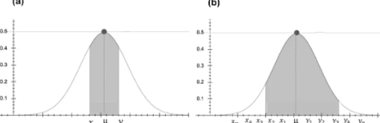
Fig. 1. The shaded area represents a range of values of attributesαjfor class ωi.(a)68%of all possible values, (b)95% of all possible values
the binary splitting approach where two candidate rule terms have to be generated for every possible attribute value (cut-point calculations) before selecting the rule term with highest conditional probability (with which it covers the target class) to be appended to the rule currently being learned. As shown in Figure 1(a), G-Prism-FB can produce a rule term in the form of
(x < α < y)by using a class conditional density probability of the Gaussian distribution function, wherexandy are valid continuous attribute values. Like in [16] x and y are set to the next closest values left and right of theµof the attribute’s values. This algorithm resulted in a better accuracy compared with original Prism that uses binary splitting with cut-point calculations to deal with a continuous attribute [13]. However, the setting ofxandydoes not explore the rule term boundaries and in fact the best rule term boundaries may lie further left and right of µ than just the next attribute values. Thus G-Prism-FB has been expanded to cover a user defined maximum number of values left and right of µ. Let k be the number of user defined values left and right of µ to be considered. The larger k the more possible rule terms will be evaluated per attribute, such as (x1 < α ≤ y3), (x3 < α ≤ y5),
(x2 < α ≤ y4),... (xn < α ≤ yk) as illustrated in Figure
1(b). This algorithm was termed G-Prism-DB. However, the larger k the more computation is required as more rule term candidates have to be evaluated.
B. Evaluation Summary of G-Prism-FB, G-Prism-DB and Prism
Both G-Prism approaches (Fixed and Dynamic) and their predecessor Prism have been evaluated empirically and com-paratively in [13] using 6 metrics and 11 datasets.
Summary of Results:
Overall, G-Prism-DB achieved a marginally better classifica-tion accuracy compared with G-Prism-FB and Prism using binary splitting except for the number of rules and abstaining rate where Prism with binary splitting performs better. The abstaining rate can be linked to the lower coverage of data instances per rule term in Prism in general. However, G-Prism-DB generated marginally fewer rules and has a lower abstaining rate compared with G-Prism-FB.
Limitations:
Please note that all here listed limitations, except limitation 5 (which is subject to future work), will be revisited in Section III which describes the proposed G-Rules-IQR algorithm.
1) Execution time:Prism and G-Prism-DB are more com-putationally expensive than G-Prism-FB as a result of frequent cut-points calculations for Prism and multiple rule term bounds evaluation for G-Prism-DB. However, as expected, both approaches of G-Prism are faster than original Prism. Please note that this evaluation metric has not been used in [13], however, it is covered in Section IV in this paper.
2) Abstaining Rate:the abstaining rate for both approaches of G-Prism is higher than the one of original Prism. This will decrease the accuracy of the classifiers despite the higher tentative accuracy values. This is because abstained instances were counted as misclassifications. 3) User defined threshold: the user has to define the
maximum number rule term boundary values to the left and right ofµ(by default six values to the left and right). However, the optimal boundary may lie beyond this user defined value and is dependent on the number of training instances. This is because the larger the number of training instances the more likely it is that there are more distinct values. Thus the larger the number of distinct values, the more likely it is that the maximum boundary is closer to µ.
4) Normal Distribution Assumption:in [13], the authors did not test the attributes’ distributions in the experiments, yet the evaluation results reflect a good performance for G-Prism-DB in most cases. However, it is still possible that G-Prism algorithms may not perform as well on attributes that are not normally distributed due to the use of GPDD.
5) Attribute Dependencies:G-Prism algorithms do not take potential dependencies between attributes into account to further improve rule quality and expressiveness. Limitations 1 to 4 are addressed in the research presented in this paper.
III. G-RULES-IQR ALGORITHM
The G-Rules-IQR approach is highlighted in Algorithm 3. The folowing subsections describe the new rule term induction procedure for continuous attributes and how the algorithm enables the induction of rule terms using GPDD, even if these attributes are not normally distributed.
A. Using GPDD to Induce Rule Terms directly from Contin-uous Attributes
The Gaussian distribution is calculated for each continuous attributeαj with meanµ and varianceσ2from all the values
associated with classification ωi. The conditional probability
for classωi is calculated using Equation 1.
P(αj|ωi) =P(αj|µ, σ2) = 1 √ 2πσ2exp(− (αj−µ)2 2σ2 ) (1) Hence, a value forP(ωi|αj)or equivalentlylog(P(ωi|αj))
Algorithm 3:Learning classification rules using G-Rules-IQR Algorithm
1 fori= 1→C do
2 D← Training Dataset;
3 while D does not contain only instances of classωi
do
4 forall attributesαj ∈D do
5 if attributeαj is categoricalthen
6 Calculate the conditional probability,
P(ωi|αj)for all possible attribute-value
(αj =x)from attributeα;
7 else if attributeαj is continuousthen
8 calculate meanµ and varianceσ2 of
continuous attributeαfor classωi ;
9 foreach value αj of attributeαdo
10 calculate P(αj|ωi)based on created
Gaussian distribution created in line 8 ;
11 end
12 Selectαj of attribute α, which has
highest value ofP(αj|ωi);
13 Compute 1st and 3rd quartile using zscore
values ;
14 zScore= 0.67 ;
15 x=σ∗(−zScore) +αj ;
16 y=σ∗(zScore) +αj ;
17 Create rule term rαin form of
(x < α≤y);
18 Calculate P(rα|ωi)
19 end
20 end
21 Select(αj=x)or (x < αj≤y)with the
maximum conditional probability as a rule term ;
22 Create a subset S from D containing all the
instances covered by selected rule term at line 21 ;
23 D←S 24 end
25 The induced rule R is a conjunction of all selected
rule terms built at line 21 ;
26 Remove all instances covered by rule R from
Training Dataset ;
27 repeat
28 lines 2 to 26 ;
29 until all instances of classωi have been removed
form the training data;
30 ResetTraining Data to its initial state ; 31 end
32 return induced Rules;
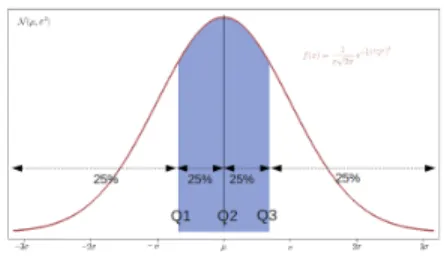
Fig. 2. Interquartile Range of Normal Random variables
used to determine the probability of a given class labelωi for
a valid value of attributeαj.
log(P(ωi|αj)) =log(P(αj|ωi)) +log(P(ωi))−log(P(αj))
(2) The created Gaussian distribution for each class label in the training data can then be used to determine the probability of an attribute value αj belonging to class label ωi, assuming
that αj lies between an upper and lower bound Ωi. This is
based on the assumption that the values close to µ represent the most common values of continuous attribute αj for ωi.
G-Rules-IQR algorithm proposed in this paper makes use of the quartiles which divide the probability density function into four parts with an equal amount of data points (25% each). As shown in Figure 2, the second quartile is identical to the median [17] while the InterQuartile Range (IQR) represents the range of attribute values that cover the middle half of the dataset. Thus, the size of coverage of this approach is dependent on the size of the datasets. We termed this G-Rules-IQR. In Particular, G-Rules-IQR uses the difference between the third and the first quartiles as in Equation 3 to find the upper rule term and the lower rule term boundaries.σ is the standard deviation from the mean, z1 is the standard score of the first quartile and is≈ −0.67while z3 is the standard score of the third quartile and is≈0.67.xusually represents the value of the mean µ but in case of data that is normally distributed it represents the highest probability density of value ofP(αj|ωi)as in lines 15 and 16 of Algorithm 3. Hence, IQR
can also be used as a simple test of whether or not data is normally distributed as the mean will be zero and the standard deviation will be equal to 1 [18]. The empirical results in Section IV-C show that our new improved approach G-Rules-IQR can resolve most of the limitations of its predecessors described in Section II-B by improving several evaluation metrics such as accuracy, tentative accuracy, execution time and F1 Score, while not requiring the user to balance rule term boundaries.
Q1= (σ∗z1) +x Q3= (σ∗z3) +x IQR=Q3−Q1
(3)
B. Transformation for Skewed Distribution
A major limitation of G-Prism-FB and G-Prism-DB algo-rithms [13] is the assumption of normally distributed attributes.
In order to overcome or mitigate this limitation, our pro-posed G-Rules-IQR algorithm incorporates a prior testing for normality for each attribute in the dataset. Hence, if values of an attribute at a particular target class are not normally distributed, then the algorithm would apply an approximate normal transformation of the attribute’s values with respect to that target class. In other words, it reduces the skewness rate of attribute values from the normal distribution. A common simple transformation for a skewed long-tailed datasets is to take the logarithm of the skewed attribute values [19]. This method of transformation to normal distribution is adopted in this paper. Every attribute in a dataset prior the application of a G-Prism classifier of G-Rules-IQR, is tested for normal distribution using one of the most popular goodness-of-fit tests called Jarque-Bera test [20] and only if it is not normally distributed, then the logarithmic transformation is applied to approximate normal distribution. G-Prism algorithms are expected to have a better performance on the transformed version of the data as their rule term induction method for continuous attributes assumes normally distributed data.
IV. COMPARATIVEEXPERIMENTALEVALUATION
The experiments in this study firstly aim to evaluate the performance of the new member of the Prism family (G-Rules-IQR) compared with its predecessors G-Prism-FB and G-Prism-DB. Unless stated otherwise the default parameters of these algorithms as stated in Section II have been used. Secondly, G-Rules-IQR and the G-Prism algorithms are com-pared with original Prism using three different discretisation methods to handle the continuous attributes indirectly. Further explanations about these versions of original Prism are given in Section IV-B. The implementation of G-Rules-IQR allowed to switch off the transformation to approximate normal distri-bution.
A. Experimental Setup
All the experiments were performed on a 2.3 GHz Intel Corei7machine with16GB DDR3 memory, running macOS High Sierra version 10.13.2. The evaluation procedure used in this experimental evaluation is hold-out procedure. All 18 datasets used in the experiments were picked randomly from the UCI repository [21], the only condition being that they contain continuous attributes and involve classification tasks. All algorithms have been implemented in the statistical programming language R [22] and re-use the same code base differing only in the methodological aspects described in this paper. The datasets have been randomly sampled without replacement into train and test datasets; whereas the test set consists of 30% the dataset and the remaining 70% was used to learn the ruleset. The datasets are described in Table I in terms of number of instances, attributes (and type of attributes) and classes. Datasets 16 and 17 contained missing values. Missing categorical values have been replaced with the most frequent categorical value for the concerning attribute, and missing continuous values have been replaced with the average value for the concerning attribute. These
metrics were Number of Rules, Abstaining Rate, F1 Score, Accuracy, Tentative Accuracy and Execution Time. Please note there is a relationship between accuracy, tentative accuracy and abstaining rate. The accuracy counts abstained instances as misclassification and tentative accuracy does not include abstained instances. Therefore the higher the abstaining rate, the lower the accuracy and the higher the tentative accuracy.
TABLE I
LIST OFDATASETS USED IN THE EXPERIMENTS
Dataset No. Instances No. Attributes No. Classes
1. iris 150 4 (cont) 3
2. seeds 210 7 (cont) 3
3. wine 178 13 (cont) 3
4. blood 748 5 (cont) 2
5. bank 1372 5 (cont) 2
6. ecoli 336 8 (7 cont, 1 name) 8 7. yeast 1484 9 (8 cont, 1 name) 10
8. page 5473 10 (cont) 5
9. model 403 5 (cont) 4
10. breast 106 10 (cont) 6
11. glass 214 10 (9 cont, 1 id) 7
12. HTRU2 17898 9 (cont) 2
13. magic 19020 11 (cont) 2
14. quality 4898 12 (cont) 11
15. letter 20000 17 (cont) 26
16. cancer 699 11 (10 cont, 1 id) 2 17. post 90 9 (8 categ, 1 cont) 3
18. EEG 14980 15 (cont) 2
B. Original Prism Incorporating Different Types of Local and Global Discretisation Methods
G-Rules-IQR was compared against original Prism with different discretisation methods explained below.
1) Prism-CutP: This extended version of Prism d [8] uses binary splitting and cup-points calculations to induce rule terms from continuous attributes.
2) Prism-ChiM: ChiMerge bottom-up global discretisation method is chosen because it is a well-known approach used to deal with continuous attributes in classification tasks [23].
3) Prism-Caim: CAIM is a top-down global discretisation algorithm that does not require user defined parameters [24]. It is determined as the interdependency between the target class and the discretisation scheme of a continuous attribute.
These variations of Prism do not assume normally dis-tributed continuous attributes, thus no transformation has been implemented for Prism using these discretisation methods.
C. Results and Interpretation
Tables II to VII show the results of the experiments with respect to 6 evaluation metrics. In each table the ‘#’ symbol refers to the number of the dataset in Table I. ‘T’ denotes that the transformation was switched on. The best result(s) in the tables for each dataset are highlighted in bold letters.
Table II shows the results for the number of rules induced. A large number of rules may be less beneficial to the human analyst compared with a well defined smaller number of rules. This is the only metric where the original version of Prism (especially Prism-CutP) clearly outperforms G-Prism algorithms and the new G-Rules-IQR algorithm. However,
what can also be seen is that the introduced G-Rules-IQR algorithm on the transformed data clearly outperforms its direct G-Prism predecessors (G-Prism-FB and G-Prism-DB) and in some cases even generates smaller rulesets than original Prism.
TABLE II NUMBER OFRULES
#
Prism G-Prism G-Rules
CutP ChiM Caim DB FB IQR
T T T 1 12 8 9 9 10 20 21 18 18 2 17 27 22 30 27 73 71 31 22 3 15 18 11 16 21 55 38 26 13 4 18 48 7 46 17 109 58 60 20 5 14 196 8 176 250 466 483 101 89 6 57 72 83 44 52 108 97 91 53 7 51 556 537 219 117 511 218 270 132 8 110 412 223 465 430 1236 1325 205 215 9 24 78 46 41 49 122 122 67 57 10 17 33 31 23 17 42 44 32 28 11 56 63 64 45 40 75 81 67 30 12 77 789 39 3928 2074 6292 7107 894 31 13 25 3929 129 3133 4563 7177 8281 3467 155 14 74 1827 1511 923 577 1576 1229 1643 171 15 868 3801 3901 843 320 2334 844 2600 875 16 33 41 37 23 6 48 9 49 11 17 30 32 31 30 30 30 30 29 29 18 37 3706 516 2602 4650 5603 7009 4585 4423
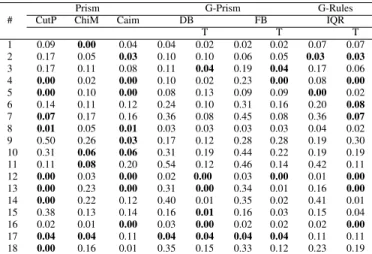
A low abstaining rate is desired as, depending on the application, abstained instances may have to be manually classified by a human analyst. Such manual labelling can be costly. In general we can observe in Table III that in most cases the abstaining rate is low for all algorithms except for a few datasets. There is no clear winner, all G-Prism versions and G-Rules-IQR are generally competitive with the original Prism versions.
TABLE III ABSTAININGRATE
#
Prism G-Prism G-Rules
CutP ChiM Caim DB FB IQR
T T T 1 0.09 0.00 0.04 0.04 0.02 0.02 0.02 0.07 0.07 2 0.17 0.05 0.03 0.10 0.10 0.06 0.05 0.03 0.03 3 0.17 0.11 0.08 0.11 0.04 0.19 0.04 0.17 0.06 4 0.00 0.02 0.00 0.10 0.02 0.23 0.00 0.08 0.00 5 0.00 0.10 0.00 0.08 0.13 0.09 0.09 0.00 0.02 6 0.14 0.11 0.12 0.24 0.10 0.31 0.16 0.20 0.08 7 0.07 0.17 0.16 0.36 0.08 0.45 0.08 0.36 0.07 8 0.01 0.05 0.01 0.03 0.03 0.03 0.03 0.04 0.02 9 0.50 0.26 0.03 0.17 0.12 0.28 0.28 0.19 0.30 10 0.31 0.06 0.06 0.31 0.19 0.44 0.22 0.19 0.19 11 0.11 0.08 0.20 0.54 0.12 0.46 0.14 0.42 0.11 12 0.00 0.03 0.00 0.02 0.00 0.03 0.00 0.01 0.00 13 0.00 0.23 0.00 0.31 0.00 0.34 0.01 0.16 0.00 14 0.00 0.22 0.12 0.40 0.01 0.35 0.02 0.41 0.01 15 0.38 0.13 0.14 0.16 0.01 0.16 0.03 0.15 0.04 16 0.02 0.01 0.00 0.03 0.00 0.02 0.02 0.02 0.00 17 0.04 0.04 0.11 0.04 0.04 0.04 0.04 0.11 0.11 18 0.00 0.16 0.01 0.35 0.15 0.33 0.12 0.23 0.19
Table IV lists the results for the F1 Score for each of the classifiers. This is the harmonic mean of precision and recall. In multi-class problems such as in these datasets, precision and recall are computed by building an average of these metrics’ values for each class. The results show that the proposed method G-Rules-IQR with transformation achieved the best
F1 Score on 11 out of 18 datasets. That is more often than any of the other evaluated algorithms. For most of the 7 datasets where the G-Rules-IQR with transformation did not achieve the best F1 Score, it was still close to the best performing F1 Score, in particular for 3 datasets it achieved an F1 Score that was at most only 3% lower than the best F1 Score. This shows that the method is competitive and in some cases even outperforms its competitors.
TABLE IV F1 SCORE
#
Prism G-Prism G-Rules
CutP ChiM Caim DB FB IQR
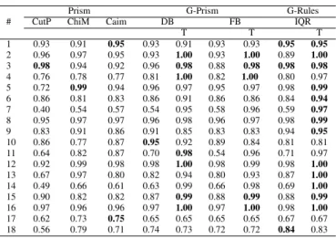
T T T 1 0.93 0.91 0.95 0.93 0.91 0.93 0.93 0.96 0.96 2 0.96 0.97 0.95 0.93 1.00 0.89 1.00 0.94 1.00 3 0.98 0.93 0.92 0.96 0.98 0.98 0.98 0.89 0.98 4 0.87 0.87 0.87 0.89 1.00 0.90 1.00 0.89 0.98 5 0.80 0.99 0.94 0.96 0.97 0.96 0.97 0.98 0.99 6 0.77 0.61 0.71 0.72 0.80 0.72 0.61 0.62 0.79 7 0.33 0.53 0.55 0.49 0.75 0.49 0.81 0.54 0.86 8 0.64 0.74 0.78 0.80 0.84 0.82 0.85 0.89 0.93 9 0.82 0.91 0.87 0.92 0.86 0.84 0.84 0.94 0.96 10 0.81 0.73 0.83 0.93 0.93 0.79 0.77 0.80 0.81 11 0.64 0.73 0.84 0.67 0.97 0.44 0.90 0.61 0.86 12 0.96 0.99 0.99 0.99 1.00 0.99 1.00 0.99 1.00 13 0.80 0.98 0.85 0.88 0.95 0.87 0.95 0.91 1.00 14 0.29 0.49 0.35 0.50 0.95 0.50 0.79 0.55 0.79 15 0.90 0.82 0.83 0.87 0.99 0.88 0.99 0.88 0.99 16 0.97 0.97 0.97 0.97 1.00 0.98 1.00 0.98 1.00 17 0.38 0.53 0.69 0.49 0.49 0.49 0.49 0.52 0.52 18 0.71 0.83 0.76 0.79 0.79 0.77 0.78 0.87 0.86 TABLE V ACCURACY #
Prism G-Prism G-Rules
CutP ChiM Caim DB FB IQR
T T T 1 0.87 0.91 0.91 0.91 0.91 0.91 0.91 0.91 0.91 2 0.92 0.95 0.94 0.86 0.90 0.87 0.95 0.87 0.97 3 0.89 0.83 0.85 0.89 0.96 0.79 0.94 0.85 0.94 4 0.76 0.77 0.77 0.77 0.98 0.77 1.00 0.77 0.97 5 0.72 0.93 0.94 0.92 0.92 0.90 0.93 0.98 0.98 6 0.77 0.75 0.75 0.72 0.85 0.65 0.77 0.73 0.91 7 0.37 0.51 0.51 0.44 0.87 0.46 0.89 0.49 0.89 8 0.95 0.95 0.96 0.95 0.97 0.95 0.97 0.96 0.98 9 0.61 0.74 0.83 0.78 0.76 0.66 0.66 0.82 0.72 10 0.59 0.72 0.81 0.66 0.78 0.50 0.69 0.66 0.66 11 0.60 0.77 0.75 0.55 0.86 0.51 0.83 0.58 0.86 12 0.92 0.97 0.98 0.97 1.00 0.96 0.99 0.98 1.00 13 0.67 0.86 0.80 0.74 0.94 0.72 0.93 0.80 1.00 14 0.49 0.63 0.58 0.56 0.98 0.59 0.97 0.60 0.99 15 0.57 0.72 0.71 0.73 0.98 0.75 0.96 0.75 0.96 16 0.96 0.95 0.96 0.94 1.00 0.96 1.00 0.96 1.00 17 0.59 0.74 0.74 0.63 0.63 0.63 0.63 0.67 0.67 18 0.56 0.75 0.70 0.67 0.71 0.66 0.72 0.77 0.77
Table V lists the results for the accuracy for each of the classifiers and abstained instances are counted as misclassi-fications. G-Rules-IQR with transformation achieved the best accuracy on 12 datasets, more often than any of the other evaluated algorithms. On 3 datasets G-Rules-IQR was not the best method, but was still very close within 3% of the best accuracy. Only on 3 datasets (9, 10 and 17) G-Rules-IQR’s accuracy was much lower than the other evaluated algorithms. However, these datasets also cause a relatively high abstaining rate.
Table VI lists the results for the tentative accuracy. In most cases the proposed method G-Rules-IQR with transforma-tion achieved the highest tentative accuracy. In particular it achieved the highest tentative accuracy on 13 out of 18 datasets and on 3 out the the remaining 5 datasets its accuracy was within 3% of the best accuracy.
TABLE VI TENTATIVEACCURACY
#
Prism G-Prism G-Rules
CutP ChiM Caim DB FB IQR
T T T 1 0.93 0.91 0.95 0.93 0.91 0.93 0.93 0.95 0.95 2 0.96 0.97 0.95 0.93 1.00 0.93 1.00 0.89 1.00 3 0.98 0.94 0.92 0.96 0.98 0.88 0.98 0.98 0.98 4 0.76 0.78 0.77 0.81 1.00 0.82 1.00 0.80 0.97 5 0.72 0.99 0.94 0.96 0.97 0.95 0.97 0.98 0.99 6 0.86 0.81 0.83 0.86 0.91 0.86 0.86 0.84 0.94 7 0.40 0.54 0.57 0.54 0.95 0.58 0.96 0.59 0.97 8 0.95 0.97 0.97 0.96 0.98 0.96 0.97 0.98 0.99 9 0.83 0.91 0.86 0.91 0.85 0.83 0.83 0.94 0.95 10 0.86 0.77 0.87 0.95 0.92 0.89 0.84 0.81 0.81 11 0.64 0.82 0.87 0.70 0.98 0.54 0.96 0.71 0.97 12 0.92 0.99 0.98 0.98 1.00 0.98 0.99 0.98 1.00 13 0.67 0.97 0.80 0.82 0.94 0.80 0.93 0.87 1.00 14 0.49 0.66 0.61 0.63 0.99 0.66 0.98 0.69 1.00 15 0.90 0.82 0.82 0.87 0.99 0.88 0.99 0.88 0.99 16 0.97 0.96 0.96 0.97 1.00 0.97 1.00 0.98 1.00 17 0.62 0.73 0.75 0.65 0.65 0.65 0.65 0.67 0.67 18 0.56 0.79 0.71 0.74 0.73 0.72 0.72 0.84 0.83
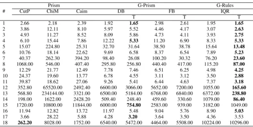
Table VII lists the results for the execution times. These also include the time needed approximating normal distribution for G-Prism classifiers and G-Rules-IQR with transforma-tion. In most cases the proposed method (G-Rules-IQR with transformation) achieved shortest execution times. On 15 out of 18 datasets it was the fastest algorithm and thus clearly outperforms its competitors. Overall the time complexity of G-Rules-IQR is expected to be similar to that of G-Prism and Prism algorithms with respect to the number of instances N
and number of attributes M. However, it is expected that G-Rules-IQR is faster. In [25] the authors estimated the worst case time complexity of a Prism classifier to be approximately O(N2M). In the worst case each rule covers exactly one data instance and each rule has two rule terms per attribute. This is a very unlikely case and time complexity is strongly dependent on the pattern in the data that can be expressed in the form of rules. The worst case of Rules-IQR and G-Prism classifiers would induce only 1 rule term per attribute and thus already divides the worst case complexity by 2. In addition G-Rules-IQR is expected to be faster than G-Prism-DB and Prism because of the number of calculations required to induce a rule term. In the worst case scenario Prism and G-Prism have to evaluate either several cut-point calculations or rule term boundaries, whereas G-Rules-IQR only has to calculate the quartiles. Also G-Rules-IQR with transformation has a lower runtime than G-Rules-IQR even though there is an additional operation. However, this is likely because IQR with transformation produces fewer rules than G-Rules-IQR without transformation in most cases.
Fig. 3. Summary of results
D. Summary of Results
Figure 3 summarises how often a particular algorithm outperformed all of its competitors relating to the evaluation measures observed in Section IV-C. It can be seen that the proposed G-Rules-IQR algorithm with transformation outper-formed its competitors in terms of F1 Score, accuracy, tentative accuracy and execution time.
V. CONCLUSION
The paper presents the rule-based G-Rules-IQR algorithm for continuous attributes, a new member of the Prism family of predictive rule induction algorithms. Previous work in this area (G-Prism-FB and G-Prism-DB) addressed the shortcoming of binary splitting to induce rule terms, which leads to rule terms covering irrelevant proportions of the training data. G-Prism-FB and G-Prism-DB generate numeric expressive rule terms using GPDD. There are 4 limitations of these methods. These are (1) more accurate G-Prism-DB has a longer execution time than G-Prism-FB, (2) both algorithms have a higher abstaining rate than the original Prism classifier, (3) G-Prism-DB requires user defined rule term boundary thresholds and (4) both approaches assume normally distributed continuous attributes. With respect to the assumption of normally distributed data, an approximation towards normally distributed data is integrated into the G-Rules-IQR algorithm. With respect to underfitting rule term boundaries, the method optimises these boundaries by removing user defined thresholds through using IQR. The approach was termed G-Rules-IQR with transformation and was evaluated empirically and comparatively with its prede-cessors including Prism with binary splitting and Prism with various well established global discretisation methods. Overall G-Rules-IQR with transformation outperformed its competi-tors with respect to F1 Score, accuracy, tentative accuracy and execution time. With regards to limitation (1), G-Rules-IQR achieves shorter execution times than its competitors, with respect to limitation (2) G-Prism achieves a competitive (similar) abstaining rate as its competitors, with respect to limitation (3) G-Rules-IQR does not require user input for rule term boundary thresholds and with respect to limitation (4) the normal distribution approximation made G-Rules-IQR the best performing Prism based classifier in this paper.
TABLE VII EXECUTIONTIME
#
Prism G-Prism G-Rules
CutP ChiM Caim DB FB IQR
T T T 1 2.66 2.18 2.39 1.92 1.65 2.98 2.61 1.95 1.65 2 3.86 12.11 8.10 5.97 5.52 4.46 4.17 3.07 2.63 3 4.93 11.27 8.52 8.09 5.86 4.73 4.11 3.93 2.75 4 6.10 15.44 7.86 12.22 5.33 11.20 6.90 8.33 5.33 5 15.07 224.80 25.31 32.70 31.64 38.50 38.78 15.64 13.48 6 10.76 18.14 22.62 9.69 6.58 8.37 6.54 7.89 5.23 7 40.37 262.30 394.20 98.40 26.08 100.20 30.32 76.20 23.60 8 1068.00 546.00 407.40 295.80 256.80 440.40 417.00 115.20 87.00 9 12.29 21.77 12.49 7.78 7.46 6.51 6.25 4.98 4.25 10 24.37 19.60 13.77 6.78 4.55 3.11 3.12 3.50 2.88 11 39.87 18.62 27.06 9.26 5.41 6.44 4.63 7.37 3.18 12 352.80 65520.00 2492.40 6600.00 3066.00 5652.00 7200.00 1055.00 165.60 13 568.80 234144.00 3321.00 6500.00 5184.00 6768.00 6840.00 6372.00 238.80 14 198.00 1622.00 2428.20 509.40 248.40 459.60 330.60 1079.00 86.40 15 1720.00 10800.00 11844.00 6000.00 754.80 2583.00 939.00 3182.00 1049.00 16 11.94 12.82 13.72 11.97 5.48 9.04 5.76 8.90 5.03 17 3.66 28.22 5.88 4.28 3.20 3.64 3.50 4.36 3.53 18 262.20 8028.00 1752.00 6540.00 5472.00 4464.00 5508.00 10224.00 10296.00
Ongoing work comprises a voting strategy for G-Rules-IQR rulesets. Currently the first rule that fires produces the prediction, however, the rule order has no relationship to the individual rule’s accuracy. Thus a rule filter and weighting mechanism (according to rule quality) is currently being inves-tigated. Also the fact that currently G-Rules-IQR does not take attribute dependencies into consideration is currently being investigated (see limitation 5 in Section II-B). For example, the expressiveness of the ruleset could be improved by not allowing rule terms of coexisting attributes in the same rule, which will lead to shorter rules and thus smaller rulesets.
REFERENCES
[1] J. Han, J. Pei, and M. Kamber,Data mining: concepts and techniques. Elsevier, 2011.
[2] K. Grbczewski, “Techniques of decision tree induction,” in Meta-Learning in Decision Tree Induction. Springer, 2014, pp. 11–117. [3] J. R. Quinlan,C4. 5: programs for machine learning. Elsevier, 2014. [4] ——, “Generating production rules from decision trees,” vol. 87, pp.
304–307, 1987.
[5] I. H. Witten, E. Frank, M. A. Hall, and C. J. Pal,Data Mining: Practical machine learning tools and techniques. Morgan Kaufmann, 2016. [6] J. Cendrowska, “Prism: An algorithm for inducing modular rules,”
International Journal of Man-Machine Studies, vol. 27, no. 4, pp. 349– 370, 1987.
[7] F. Stahl and M. Bramer, “Computationally efficient induction of classifi-cation rules with the pmcri and j-pmcri frameworks,”Knowledge-Based Systems, vol. 35, pp. 49–63, 2012.
[8] M. Bramer,Principles of data mining. Springer, 2007, vol. 180. [9] W. W. Cohen, “Fast effective rule induction,” in Machine Learning
Proceedings 1995. Elsevier, 1995, pp. 115–123.
[10] P. Clark and T. Niblett, “The cn2 induction algorithm,”Machine learn-ing, vol. 3, no. 4, pp. 261–283, 1989.
[11] J. F¨urnkranz, D. Gamberger, and N. Lavraˇc,Foundations of rule learn-ing. Springer Science & Business Media, 2012.
[12] M. Bramer, “An information-theoretic approach to the pre-pruning of classification rules,” inInternational Conference on Intelligent Informa-tion Processing. Springer, 2002, pp. 201–212.
[13] M. Almutairi, F. Stahl, and M. Bramer, “Improving modular classifica-tion rule inducclassifica-tion with g-prism using dynamic rule term boundaries,” inInternational Conference on Innovative Techniques and Applications of Artificial Intelligence. Springer, 2017, pp. 115–128.
[14] M. Almutairi, F. Stahl, M. Jennings, T. Le, and M. Bramer, “Towards expressive modular rule induction for numerical attributes,” inResearch
and Development in Intelligent Systems XXXIII: Incorporating Applica-tions and InnovaApplica-tions in Intelligent Systems XXIV. Springer, 2016, pp. 229–235.
[15] M. Bramer, “Automatic induction of classification rules from examples using n-prism,” inResearch and development in intelligent systems XVI. Springer, 2000, pp. 99–121.
[16] T. Le, F. Stahl, J. B. Gomes, M. M. Gaber, and G. Di Fatta, “Computa-tionally efficient rule-based classification for continuous streaming data,” inResearch and Development in Intelligent Systems XXXI. Springer, 2014, pp. 21–34.
[17] C. Walck, “Hand-book on statistical distributions for experimentalists,” Tech. Rep., 1996.
[18] L. Statistics. [Online]. Available: https://statistics.laerd.com [19] H. C. Thode,Testing for normality. CRC press, 2002, vol. 164. [20] C. M. Jarque and A. K. Bera, “Efficient tests for normality,
homoscedas-ticity and serial independence of regression residuals,”Economics let-ters, vol. 6, no. 3, pp. 255–259, 1980.
[21] D. N. A. Asuncion, “UCI machine learning repository,” 2007. [Online]. Available: http://www.ics.uci.edu/∼mlearn/MLRepository.html [22] R Development Core Team, R: A Language and Environment
for Statistical Computing, R Foundation for Statistical Computing, Vienna, Austria, 2008, ISBN 3-900051-07-0. [Online]. Available: http://www.R-project.org
[23] R. Kerber, “Chimerge: Discretization of numeric attributes,” in Proceed-ings of the tenth national conference on Artificial intelligence. Aaai Press, 1992, pp. 123–128.
[24] L. A. Kurgan and K. J. Cios, “Caim discretization algorithm,” IEEE transactions on Knowledge and Data Engineering, vol. 16, no. 2, pp. 145–153, 2004.
[25] F. Stahl, D. May, H. Mills, M. Bramer, and M. M. Gaber, “A scalable ex-pressive ensemble learning using random prism: a mapreduce approach,”
Transactions on Large-Scale Data- and Knowledge-Centered Systems, vol. 9070, pp. 90–107, 2015.