Text Segmentation for MRC Document Compression
Eri Haneda
, Student Member, IEEE
, and Charles A. Bouman
, Fellow, IEEE
Abstract—The mixed raster content (MRC) standard (ITU-T T.44) specifies a framework for document compression which can dramatically improve the compression/quality tradeoff as compared to traditional lossy image compression algorithms. The key to MRC compression is the separation of the document into foreground and background layers, represented as a binary mask. Therefore, the resulting quality and compression ratio of a MRC document encoder is highly dependent upon the segmentation algorithm used to compute the binary mask. In this paper, we pro-pose a novel multiscale segmentation scheme for MRC document encoding based upon the sequential application of two algorithms. The first algorithm, cost optimized segmentation (COS), is a blockwise segmentation algorithm formulated in a global cost opti-mization framework. The second algorithm, connected component classification (CCC), refines the initial segmentation by classifying feature vectors of connected components using an Markov random field (MRF) model. The combined COS/CCC segmentation algo-rithms are then incorporated into a multiscale framework in order to improve the segmentation accuracy of text with varying size. In comparisons to state-of-the-art commercial MRC products and selected segmentation algorithms in the literature, we show that the new algorithm achieves greater accuracy of text detection but with a lower false detection rate of nontext features. We also demonstrate that the proposed segmentation algorithm can improve the quality of decoded documents while simultaneously lowering the bit rate.
Index Terms—Document compression, image segmentation, Markov random fields, MRC compression, Multiscale image analysis.
I. INTRODUCTION
W
ITH the wide use of networked equipment such as com-puters, scanners, printers and copiers, it has become more important to efficiently compress, store, and transfer large document files. For example, a typical color document scanned at 300 dpi requires approximately 24 M bytes of storage without compression. While JPEG and JPEG2000 are frequently used tools for natural image compression, they are not very effec-tive for the compression of raster scanned compound documents which typically contain a combination of text, graphics, and nat-ural images. This is because the use of a fixed DCT or wavelet transformation for all content typically results in severe ringing distortion near edges and line-art.The mixed raster content (MRC) standard is a framework for layer-based document compression defined in the ITU-T T.44 [1] that enables the preservation of text detail while reducing
Manuscript received January 23, 2010; revised July 06, 2010; accepted De-cember 02, 2010. Date of publication DeDe-cember 23, 2010; date of current ver-sion May 18, 2011. This work was supported by Samsung Electronics. The as-sociate editor coordinating the review of this manuscript and approving it for publication was Dr. Maya R. Gupta.
The authors are with the School of Electrical and Computer Engineering, Purdue University, West Lafayette, IN 47907-2035 USA (e-mail: ehaneda@ecn. purdue.edu; [email protected]).
Color versions of one or more of the figures in this paper are available online at http://ieeexplore.ieee.org.
Digital Object Identifier 10.1109/TIP.2010.2101611
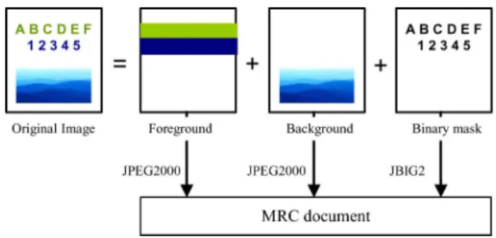
Fig. 1. Illustration of MRC document compression standard mode 1 structure. An image is divided into three layers: a binary mask layer, foreground layer, and background layer. The binary mask indicates the assignment of each pixel to the foreground layer or the background layer by a “1” (black) or “0” (white), respectively. Typically, text regions are classified as foreground while picture regions are classified as background. Each layer is then encoded independently using an appropriate encoder.
the bitrate of encoded raster documents. The most basic MRC approach, MRC mode 1, divides an image into three layers: a binary mask layer, foreground layer, and background layer. The binary mask indicates the assignment of each pixel to the foground layer or the backfoground layer by a “1” or “0” value, re-spectively. Typically, text regions are classified as foreground while picture regions are classified as background. Each layer is then encoded independently using an appropriate encoder. For example, foreground and background layers may be encoded using traditional photographic compression such as JPEG or JPEG2000 while the binary mask layer may be encoded using symbol-matching based compression such as JBIG or JBIG2. Moreover, it is often the case that different compression ratios and subsampling rates are used for foreground and background layers due to their different characteristics. Typically, the fore-ground layer is more aggressively compressed than the back-ground layer because the foreback-ground layer requires lower color and spatial resolution. Fig. 1 shows an example of layers in an MRC mode 1 document.
Perhaps the most critical step in MRC encoding is the seg-mentation step, which creates a binary mask that separates text and line-graphics from natural image and background regions in the document. Segmentation influences both the quality and bitrate of an MRC document. For example, if a text compo-nent is not properly detected by the binary mask layer, the text edges will be blurred by the background layer encoder. Alter-natively, if nontext is erroneously detected as text, this error can also cause distortion through the introduction of false edge ar-tifacts and the excessive smoothing of regions assigned to the foreground layer. Furthermore, erroneously detected text can also increase the bit rate required for symbol-based compres-sion methods such as JBIG2. This is because erroneously de-tected and unstructure nontext symbols are not be efficiently represented by JBIG2 symbol dictionaries.
Many segmentation algorithms have been proposed for ac-curate text extraction, typically with the application of optical character recognition (OCR) in mind. One of the most popular top-down approaches to document segmentation is the – cut algorithm [2] which works by detecting white space using hor-izontal and vertical projections. The run length smearing algo-rithm (RLSA) [3], [4] is a bottom-up approach which basically uses region growing of characters to detect text regions, and the Docstrum algorithm proposed in [5] is another bottom-up method which uses -nearest neighbor clustering of connected components. Chen et. al recently developed a multiplane based segmentation method by incorporating a thresholding method [6]. A summary of the algorithms for document segmentation can be found in [7]–[11].
Perhaps the most traditional approach to text segmentation is Otsu’s method [12] which thresholds pixels in an effort to divide the document’s histogram into objects and background. There are many modified versions of Otsu’s method [6], [13]. While Otsu uses a global thresholding approach, Niblack [14] and Sauvola [15] use a local thresholding approach. Kapur’s method [16] uses entropy information for the global thresh-olding, and Tsai [17] uses a moment preserving approach. A comparison of the algorithms for text segmentation can be found in [18].
In order to improve text extraction accuracy, some text seg-mentation approaches also use character properties such as size, stroke width, directions, and run-length histogram [19]–[22]. Other binarization approaches for document coding have used rate-distortion minimization as a criteria for document binariza-tion [23], [24].
Many recent approaches to text segmentation have been based upon statistical models. One of the best commercial text segmentation algorithms, which is incorporated in the DjVu document encoder, uses a hidden Markov model (HMM) [25], [26]. The DjVu software package is perhaps the most popular MRC-based commercial document encoder. Although there are other MRC-based encoders such as LuraDocument [27], we have found DjVu to be the most accurate and robust algorithm available for document compression. However, as a commercial package, the full details of the DjVu algorithm are not available. Zhenget al.[28] used an MRF model to exploit the contextual document information for noise removal. Similarly, Kumar [29]et al.used an MRF model to refine the initial segmentation generated by the wavelet analysis. J. G. Kuket al.and Caoet al. also developed a MAP-MRF text segmentation framework which incorporates their proposed prior model [30], [31].
Recently, a conditional random field (CRF) model, originally proposed by Lafferty [32], has attracted interest as an improved model for segmentation. The CRF model differs from the tradi-tional MRF models in that it directly models the posterior distri-bution of labels given observations. For this reason, in the CRF approach the interactions between labels are a function of both labels and observations. The CRF model has been applied to dif-ferent types of labeling problems including blockwise segmen-taion of manmade structures [33], natural image segmentation [34], and pixelwise text segmentation [35].
In this paper, we present a robust multiscale segmentation al-gorithm for both detecting and segmenting text in complex
doc-uments containing background gradations, varying text size, re-versed contrast text, and noisy backgrounds. While consider-able research has been done in the area of text segmentation, our approach differs in that it integrates a stochastic model of text structure and context into a multiscale framework in order to best meet the requirements of MRC document compression. Accordingly, our method is designed to minimize false detec-tions of unstructured nontext components (which can create ar-tifacts and increase bit-rate) while accurately segmenting true-text components of varying size and with varying backgrounds. Using this approach, our algorithm can achieve higher decoded image quality at a lower bit-rate than generic algorithms for doc-ument segmentation. We note that a preliminary version of this approach, without the use of an MRF prior model, was presented in the conference paper of [36], and that the source code for the method described in this paper is publicly available.1
Our segmentation method is composed of two algorithms that are applied in sequence: the cost optimized segmentation (COS) algorithm and the connected component classification (CCC) gorithm. The COS algorithm is a blockwise segmentation al-gorithm based upon cost optimization. The COS produces a binary image from a gray level or color document; however, the resulting binary image typically contains many false text detections. The CCC algorithm further processes the resulting binary image to improve the accuracy of the segmentation. It does this by detecting nontext components (i.e., false text detec-tions) in a Bayesian framework which incorporates an Markov random field (MRF) model of the component labels. One im-portant innovation of our method is in the design of the MRF prior model used in the CCC detection of text components. In particular, we design the energy terms in the MRF distribution so that they adapt to attributes of the neighboring components’ relative locations and appearance. By doing this, the MRF can enforce stronger dependencies between components which are more likely to have come from related portions of the document. The organization of this paper is as follows. In Section II and Section III, we describe COS and CCC algorithms. We also de-scribe the multiscale implementation in Section IV. Section V presents experimental results, in both quantitative and qualita-tive ways.
II. COS
The COS algorithm is a block-based segmentation algorithm formulated as a global cost optimization problem. The COS al-gorithm is comprised of two components: blockwise segmenta-tion and global segmentasegmenta-tion. The blockwise segmentasegmenta-tion di-vides the input image into overlapping blocks and produces an initial segmentation for each block. The global segmentation is then computed from the initial segmented blocks so as to mini-mize a global cost function, which is carefully designed to favor segmentations that capture text components. The parameters of the cost function are optimized in an offline training procedure. A block diagram for COS is shown in Fig. 2.
A. Blockwise Segmentation
Blockwise segmentation is performed by first dividing the image into overlapping blocks, where each block contains
Fig. 2. COS algorithm comprises two steps: blockwise segmentation and global segmentation. The parameters of the cost function used in the global segmentation are optimized in an offline training procedure.
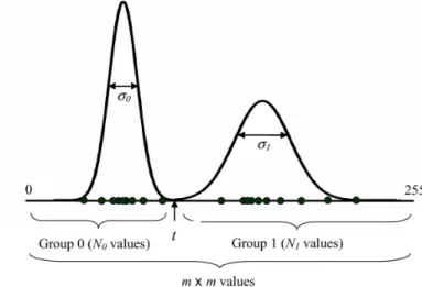
Fig. 3. Illustration of a blockwise segmentation. The pixels in each block are separated into foreground (“1”) or background (“0”) by comparing each pixel with a thresholdt. The thresholdtis then selected to minimize the total subclass variance.
pixels, and adjacent blocks overlap by pixels in both the horizontal and vertical directions. The blocks are denoted
by for , and , where and
are the number of the blocks in the vertical and horizontal di-rections, respectively. If the height and width of the input image is not divisible by , the image is padded with zeros. For each block, the color axis having the largest variance over the block is selected and stored in a corresponding gray image block, .
The pixels in each block are segmented into foreground (“1”) or background (“0”) by the clustering method of Cheng and Bouman [24]. The clustering method classifies each pixel in by comparing it to a threshold . This threshold is selected to minimize the total subclass variance. More specifically, the minimum value of the total subclass variance is given by
(1) where and are number of pixels classified as 0 and 1 in by the threshold , and and are the variances within each subclass (see Fig. 3). Note that the subclass vari-ance can be calculated efficiently. First, we create a histogram by counting the number of pixels which fall into each value be-tween 0 and 255. For each threshold , we can recur-sively calculate and from the values calculated for the previous threshold of . The threshold that minimizes the subclass variance is then used to produce a binary segmentation
of the block denoted by .
Fig. 4. Illustration of class definition for each block. Black indicates a label of “1” (foreground) and white indicates a label of “0” (background). Four seg-mentation result candidates are defined; original (class 0), reversed (class 1), all background (class 2), and all foreground (class 3). The final segmentation will be one of these candidates. In this example, block size ism = 6.
B. Global Segmentation
The global segmentation step integrates the individual seg-mentations of each block into a single consistent segmentation of the page. To do this, we allow each block to be modified using a class assignment denoted by,
Original Reversed
All background All foreground (2) Notice that for each block, the four possible values of correspond to four possible changes in the block’s segmenta-tion: original, reversed, all background, or all foreground. If the block class is “original,” then the original binary segmentation of the block is retained. If the block class is “reversed,” then the assignment of each pixel in the block is reversed (i.e., 1 goes to 0, or 0 goes to 1). If the block class is set to “all background” or “all foreground,” then the pixels in the block are set to all 0’s or all 1’s, respectively. Fig. 4 illustrates an example of the four possible classes where black indicates a label of “1” (fore-ground) and white indicates a label of “0” (back(fore-ground).
Our objective is then to select the class assignments, , so that the resulting binary masks, , are consis-tent. We do this by minimizing the following global cost as a function of the class assignments, for all ,
(3) As it is shown, the cost function contains four terms, the first term representing the fit of the segmentation to the image pixels, and the next three terms representing regularizing constraints on the segmentation. The values , , and are then model pa-rameters which can be adjusted to achieve the best segmentation quality.
The first term is the square root of the total subclass vari-ation within a block given the assumed segmentvari-ation. More specifically
if
, if (4)
where is the standard deviation of all the pixels in the block. Since must always be less than or equal to , the term can always be reduced by choosing a finer segmentation corre-sponding to or 1 rather than smoother segmentation corresponding to or 3.
The terms and regularize the segmentation by penal-izing excessive spatial variation in the segmentation. To com-pute the term , the number of segmentation mismatches be-tween pixels in the overlapping region bebe-tween block and the horizontally adjacent block is counted. The term is then calculated as the number of the segmentation mismatches divided by the total number of pixels in the overlapping region. Also is similarly defined for vertical mismatches. By min-imizing these terms, the segmentation of each block is made consistent with neighboring blocks.
The term denotes the number of the pixels classified as foreground (i.e., “1”) in divided by the total number of pixels in the block. This cost is used to ensure that most of the area of image is classified as background.
For computational tractability, the cost minimization is itera-tively performed on individual rows of blocks, using a dynamic programming approach [37]. Note that row-wise approach does not generally minimize the global cost function in one pass through the image. Therefore, multiple iterations are performed from top to bottom in order to adequately incorporate the vertical consistency term. In the first iteration, the optimization of th row incorporates the term containing only the th row. Starting from the second iteration, terms for both the th row and th row are included. The optimization stops when no changes occur to any of the block classes. Experimentally, the sequence of updates typically converges within 20 iterations.
The cost optimization produces a set of classes for overlap-ping blocks. Since the output segmentation for each pixel is am-biguous due to the block overlap, the final COS segmentation output is specified by the center region of each
overlapping block.
The weighting coefficients , , and were found by minimizing the weighted error between segmentation results of training images and corresponding ground truth segmentations. A ground truth segmentation was generated manually by cre-ating a mask that indicates the text in the image. The weighted error criteria which we minimized is given by
(5)
where , and the terms and
are the number of pixels in the missed de-tection and false dede-tection categories, respectively. For our application, the missed detections are generally more serious than false detections, so we used a value of which more heavily weighted miss detections. In Section III, we
Fig. 5. Illustration of how the component inversion step can correct erroneous segmentations of text. (a) Original document before segmentation. (b) Result of COS binary segmentation. (c) Corrected segmentation after component inversion.
will show how the resulting false detections can be effectively reduced.
III. CCC
The CCC algorithm refines the segmentation produced by COS by removing many of the erroneously detected nontext components. The CCC algorithm proceeds in three steps: con-nected component extraction, component inversion, and com-ponent classification. The connected comcom-ponent extraction step identifies all connected components in the COS binary segmen-tation using a 4-point neighborhood. In this case, connected components less than six pixels were ignored because they are nearly invisible at 300 dpi resolution. The component inversion step corrects text segmentation errors that sometimes occur in COS segmentation when text is locally embedded in a high-lighted region [see Fig. 5(a)]. Fig. 5(b) illustrates this type of error where text is initially segmented as background. Notice the text “100 Years of Engineering Excellence” is initially seg-mented as background due to the red surrounding region. In order to correct these errors, we first detect foreground nents that contain more than eight interior background compo-nents (holes). In each case, if the total number of interior back-ground pixels is less than half of the surrounding foreback-ground pixels, the foreground and background assignments are inverted. Fig. 5(c) shows the result of this inversion process. Note that this type of error is a rare occurrence in the COS segmentation.
The final step of component classification is performed by extracting a feature vector for each component, and then com-puting a MAP estimate of the component label. The feature vector, , is calculated for each connected component, , in the COS segmentation. Each is a 4-D feature vector which de-scribes aspects of the th connected component including edge
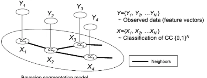
Fig. 6. Illustration of a Bayesian segmentation model. Line segments indicate dependency between random variables. Each componentCC has an observed feature vector,y, and a class label,x 2 f0; 1g. Neighboring pairs are indi-cated by thick line segments.
depth and color uniformity. Finally, the feature vector is used to determine the class label, , which takes a value of 0 for non-text and 1 for non-text.
The Bayesian segmentation model used for the CCC algo-rithm is shown in Fig. 6. The conditional distribution of the fea-ture vector given is modeled by a multivariate Gaussian mixture while the underlying true segmentation labels are mod-eled by an MRF. Using this model, we classify each component by calculating the MAP estimate of the labels, , given the fea-ture vectors, . In order to do this, we first determine which components are neighbors in the MRF. This is done based upon the geometric distance between components on the page. A. Statistical Model
Here, we describe more details of the statistical model used for the CCC algorithm. The feature vectors for “text” and “non-text” groups are modeled as -dimensional multivariate Gaussian mixture distributions
(6) where is a class label of nontext or text for the th connected component. The and are the number of clusters in each Gaussian mixture distribution, and the , , and are the mean, covariance matrix, and weighting coefficient of the th cluster in each distribution. In order to simplify the data model, we also assume that the values are conditionally independent given the associated values .
(7) The components of the feature vectors include measurements of edge depth and external color uniformity of the th connected component. The edge depth is defined as the Euclidean distance between RGB values of neighboring pixels across the compo-nent boundary (defined in the initial COS segmentation). The color uniformity is associated with the variation of the pixels outside the boundary. In this experiment, we defined a feature
vector with four components, ,
where the first two are mean and variance of the edge depth and
the last two are the variance and range of external pixel values. More details are provided in the Appendix.
To use an MRF, we must define a neighborhood system. To do this, we first find the pixel location at the center of mass for each connected component. Then for each component we search out-ward in a spiral pattern until the nearest neighbors are found. The number is determined in an offline training process along with other model parameters. We will use the symbol to de-note the set of neighbors of connected component . To ensure all neighbors are mutual (which is required for an MRF), if com-ponent is a neighbor of component (i.e., ), we add component to the neighbor list of component (i.e., ) if this is not already the case.
In order to specify the distribution of the MRF, we first define augmented feature vectors. The augmented feature vector, , for the th connected component consists of the feature vector concatenated with the horizontal and vertical pixel location of the connected component’s center. We found the location of connected components to be extremely valuable contextual in-formation for text detection. For more details of the augmented feature vector, see the Appendix.
Next, we define a measure of dissimilarity between connected components in terms of the Mahalanobis distance of the aug-mented feature vectors given by
(8) where is the covariance matrix of the augmented feature vec-tors on training data. Next, the Mahalanobis distance, , is normalized using the equations
(9)
where is averaged distance between the th connected com-ponent and all of its neighbors, and is similarly defined. This normalized distance satisfies the symmetry property, that
is .
Using the defined neighborhood system, we adopted an MRF model with pair-wise cliques. Let be the set of all where
and denote neighboring connected components. Then, the are assumed to be distributed as
(10)
(11) where is an indicator function taking the value 0 or 1, and , , and are scalar parameters of the MRF model. As we can see, the classification probability is penalized by the number of neighboring pairs which have different classes. This number is also weighted by the term . If there exists a similar neighbor close to a given component, the term becomes large since
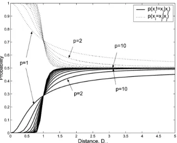
Fig. 7. Illustration of classification probability ofx given a single neighborx as a function of the distance between the two components. The solid line shows a graph ofp(x 6= x jx )while the dashed line shows a graph ofp(x = x jx ). The parameters are set toa = 0:1andb = 1:0.
is small. This favors increasing the probability that the two similar neighbors have the same class.
Fig. 7 illustrates the classification probability of given a single neighbor as a function of the distance between the two components . Here, we assume the classification of is given. The solid line shows a graph of the probability
while the dashed line shows a graph of the probability . Note that the parameter controls the rolloff of the function, and and control the minimum and transition point for the function. The actual parameters, , are optimized in an offline training procedure (see Section III-B).
With the MRF model defined previously, we can compute a maximuma posteriori(MAP) estimate to find the optimal set
of classification labels . The MAP
estimate is given by
(12) We introduced a term to control the tradeoff between missed and false detections. The term may take a positive or negative value. If is positive, both text detections and false detections increase. If it is negative, false and missed detections are reduced.
To find an approximate solution of (12), we use iterative conditional modes (ICM) which sequentially minimizes the local posterior probabilities [38], [39]. The classification labels, , are initialized with their maximum likelihood (ML) estimates, and then the ICM procedure iterates through the set of classification labels until a stable solution is reached. B. Parameter Estimation
In our statistical model, there are two sets of parameters to be estimated by a training process. The first set of
parame-ters comes from the -dimensional multivariate Gaussian mix-ture distributions given by (6) which models the feamix-ture vec-tors from text and nontext classes. The second set of parameters, , controls the MRF model of (11). All parameters are estimated in an offline procedure using a training image set and their ground truth segmentations. The training images were first segmented using the COS algorithm. All foreground con-nected components were extracted from the resulting segmen-tations, and then each connected component was labeled as text or nontext by matching to the components on the ground truth segmentations. The corresponding feature vectors were also cal-culated from the original training images.
The parameters of the Gaussian mixture distribution were es-timated using the EM algorithm [40]. The number of clusters in each Gaussian mixture for text and nontext were also de-termined using the minimum description length (MDL) esti-mator [41].
The prior model parameters were inde-pendently estimated using pseudolikelihood maximization [42]–[44]. In order to apply pseudolikelihood estimation, we must first calculate the conditional probability of a classification label given its neighboring components’ labels
(13)
where the normalization factor is defined by
(14)
Therefore, the pseudolikelihood parameter estimation for our case is
(15)
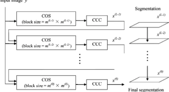
IV. MULTISCALE-COS/CCC SEGMENTATIONSCHEME
In order to improve accuracy in the detection of text with varying size, we incorporated a multiscale framework into the COS/CCC segmentation algorithm. The multiscale framework allows us to detect both large and small components by com-bining results from different resolutions [45]–[47]. Since the COS algorithm uses a single block size (i.e., single scale), we found that large blocks are typically better suited for detecting large text, and small blocks are better suited for small text. In order to improve the detection of both large and small text, we use a multiscale segmentation scheme which uses the results of coarse-scale segmentations to guide segmentation on finer scales. Note that both COS and CCC segmentations are
per-Fig. 8. Illustration of a multiscale-COS/CCC algorithm. Segmentation pro-gresses from coarse to fine scales, incorporating the segmentation result from the previous coarser scale. Both COS and CCC are performed on each scale, however only COS was adapted to the multiscale scheme.
formed on each scale, however, only COS is adapted to the mul-tiscale scheme.
Fig. 8 shows the overview of our multiscale-COS/CCC scheme. In the multiscale scheme, segmentation progresses from coarse to fine scales, where the coarser scales use larger block sizes, and finer scales use smaller block sizes. Each scale is numbered from to 0, where is the coarsest scale and 0 is the finest scale. The COS algorithm is modified to use different block sizes for each scale (denoted as ), and incorporates the previous coarser segmentation result by adding a new term to the cost function.
The new cost function for the multiscale scheme is shown in (16). It is a function of the class assignments on both the th and th scale
(16) where denotes the term for the th scale, and is the set of class assignments for the scale, that is for all , . The term is a set of pixels in a block at the position , and the term is the segmentation result for the block.
As it is shown in the equation, this modified cost function incorporates a new term that makes the segmentation con-sistent with the previous coarser scale. The term , is defined as the number of mismatched pixels within the block be-tween the current scale segmentation and the previous coarser scale segmentation . The exception is that only the pixels that switch from “1” (foreground) to “0” (background) are counted when or . This term encour-ages a more detailed segmentation as we proceed to finer scales. The term is normalized by dividing by the block size on the current scale. Note that the term is ignored for the coarsest scale. Using the new cost function, we find the class
assign-ments, , for each scale.
The parameter estimation of the cost function for is performed in an offline task. The goal is to find the optimal parameter set
for . To simplify the optimization
process, we first performed single scale optimization to
find for each scale. Then, we
found the optimal set of given the
. The error to be minimized was the number of mismatched pixels compared to ground truth segmentations, as shown in (5). The , the weighting factor of the error for false detection, was fixed to 0.5 for the multiscale-COS/CCC training process.
V. RESULTS
In this section, we compare the multiscale-COS/CCC, COS/CCC, and COS segmentation results with the results of two popular thresholding methods, an MRF-based segmenta-tion method, and two existing commercial software packages which implement MRC document compression. The thresh-olding methods used for the comparison in this study are Otsu [12] and Tsai [17] methods. These algorithms showed the best segmentation results among the thresholding methods in [12], [14]–[16], and [17]. In the actual comparison, the sRGB color image was first converted to a luma grayscale image, then each thresholding method was applied. For “Otsu/CCC” and “Tsai/CCC,” the CCC algorithm was combined with the Otsu and Tsai binarization algorithms to remove false detections. In this way, we can compare the end result of the COS algorithm to alternative thresholding approaches.
The MRF-based binary segmentation used for the compar-ison is based upon the MRF statistical model developed by Zheng and Doermann [28]. The purpose of their algorithm is to classify each component as either noise, hand-written text, or machine printed text from binary image inputs. Due to the complexity of implementation, we used a modified version of the CCC algorithm incorporating their MRF model by simply replacing our MRF classification model by their MRF noise classification model. The multiscale COS algorithm was applied without any change. The clique frequencies of their model were calculated through offline training using a training data set. Other parameters were set as proposed in the paper.
We also used two commercial software packages for the comparison. The first package is the DjVu implementation contained in Document Express Enterprise version 5.1 [48]. DjVu is commonly used software for MRC compression and produces excellent segmentation results with efficient com-putation. By our observation, version 5.1 produces the best segmentation quality among the currently available DjVu pack-ages. The second package is LuraDocument PDF Compressor, Desktop Version [27]. Both software packages extract text to create a binary mask for layered document compression.
The performance comparisons are based primarily upon two aspects: the segmentation accuracy and the bitrate resulting from JBIG2 compression of the binary segmentation mask. We show samples of segmentation output and MRC decoded images using each method for a complex test image. Finally, we list the computational run times for each method.
A. Preprocessing
For consistency all scanner outputs were converted to sRGB color coordinates [49] and descreened [50] before segmentation. The scanned RGB values were first converted to an intermediate
TABLE I
PARAMETERSETTINGS FOR THECOS ALGORITHM INMULTISCALE-COS/CCC
device-independent color space, CIE XYZ, then transformed to sRGB [51]. Then, resolution synthesis-based denoising (RSD) [50] was applied. This descreening procedure was applied to all of the training and test images. For a fair comparison, the test images which were fed to other commercial segmentation software packages were also descreened by the same procedure. B. Segmentation Accuracy and Bitrate
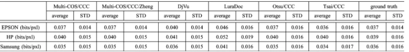
To measure the segmentation accuracy of each algorithm, we used a set of scanned documents along with corresponding “ground truth” segmentations. First, 38 documents were chosen from different document types, including flyers, newspapers, and magazines. The documents were separated into 17 training images and 21 test images, and then each document was scanned at 300 dots per inch (dpi) resolution on the EPSON STYLUS PHOTO RX700 scanner. After manually segmenting each of the scanned documents into text and nontext to create ground truth segmentations, we used the training images to train the al-gorithms, as described in the previous sections. The remaining test images were used to verify the segmentation quality. We also scanned the test documents on two additional scanners: the HP Photosmart 3300 All-in-One series and Samsung SCX-5530 FN. These test images were used to examine the robustness of the algorithms to scanner variations.
The parameter values used in our results are as follows. The optimal parameter values for the multiscale-COS/CCC were shown in the Table I. Three layers were used for multi-scale-COS/CCC algorithm, and the block sizes were 36 36, 72 72, and 144 144. The parameters for the CCC algorithm
were , , . The number of
neighbors in the -NN search was 6. In DjVu, the segmentation threshold was set to the default value while LuraDocument had no adjustable segmentation parameters.
To evaluate the segmentation accuracy, we measured the per-cent of missed detections and false detections of segmented components, denoted as and . More specifically, and were computed in the following manner. The text in ground truth images were manually segmented to produce components. For each of these ground truth components, the corresponding location in the test segmentation was searched for a symbol of the same shape. If more than 70% of the pixels matched in the binary pattern, then the symbol was considered detected. If the total number of correctly detected components is , then we define that the fraction of missed components as (17) Next, each correctly detected component was removed from the segmentation, and the number of remaining false components,
, in the segmentation was counted. The fraction of false components is defined as
(18) We also measured the percent of missed detections and false detections of individualpixels, denoted as and . They were computed similarly to the and defined previously, except the number of pixels in the missed detections and false detections were counted, and these numbers were then divided by the total number of pixels in the ground truth document
(19) (20) Table II shows the segmentation accuracy of our algorithms (multiscale-COS/CCC, COS/CCC, and COS), the thresholding methods (Otsu and Tsai), an MRF-based algorithm (multiscale-COS/CCC/Zheng), and two commercial MRC document com-pression packages (DjVu and LuraDocument). The values in the Table II were calculated from all of the available test im-ages from each scanner. Notice that multiscale-COS/CCC ex-hibits quite low error rate in all categories, and shows the lowest error rate in the missed component detection error . For the missed pixel detection , both multiscale-COS/CCC/Zheng and the multiscale-COS/CCC show the first and second lowest error rates. For the false detections and , the thresh-olding methods such as Otsu and Tsai exhibit the low error rates, however those thresholding methods show a high missed detec-tion error rate. This is because the thresholding methods cannot separate text from background when there are multiple colors represented in the text.
For the internal comparisons among our algorithms, we observed that CCC substantially reduces the of the COS al-gorithm without increasing the . The multiscale-COS/CCC segmentation achieves further improvements and yields the smallest among our methods. Note that the missed pixel detection error rate in the multiscale-COS/CCC is partic-ularly reduced compared to the other methods. This is due to the successful detection of large text components along with small text detection in the multiscale-COS/CCC. Large text influences more than small text since each symbol has a large number of pixels.
In the comparison of multiscale-COS/CCC to commercial products DjVu and LuraDocument, the multiscale-COS/CCC exhibits a smaller missed detection error rate in all categories. The difference is most prominent in the false detection error rates ( , ).
Fig. 9 shows the tradeoff between missed detection and false detection, versus and versus , for the multiscale-COS/CCC, multiscale-COS/CCC/Zheng, and DjVu. All three methods employ a statistical model such as an MRF or HMM for text detection. In DjVu, the tradeoff be-tween missed detection and false detection was controlled by adjustment of sensitivity levels. In multiscale-COS/CCC and
TABLE II
SEGMENTATIONACCURACYCOMPARISONBETWEEN OURALGORITHMS(MULTI-COS/CCC, COS/CCC,ANDCOS), THRESHOLDINGALGORITHMS(OTSU AND TSAI),ANMRF-BASEDALGORITHM(MULTISCALE-COS/CCC/ZHENG),ANDTWOCOMMERCIALMRC DOCUMENTCOMPRESSIONPACKAGES(DJVU AND
LURADOCUMENT). MISSEDCOMPONENTERROR,p ,THECORRESPONDINGMISSEDPIXELERROR,p , FALSECOMPONENTERROR,p ,AND THE CORRESPONDINGFALSEPIXELERROR,p ,ARECALCULATED FOREPSON, HP,ANDSAMSUNGSCANNEROUTPUT
Fig. 9. Comparison of multiscale-COS/CCC, multiscale-COS/CCC/Zheng, and DjVu in tradeoff between missed detection error versus false detection error. (a) Tradeoff betweenp andp . (b) Tradeoff betweenp andp .
TABLE III
COMPARISON OFBITRATEBETWEENMULTISCALE-COS/CCC, MULTISCALE-COS/CCC/ZHENG, DJVU, LURADOCUMENT, OTSU/CCC,AND TSAI/CCCFORJBIG2 COMPRESSEDBINARYMASKLAYER FORIMAGESSCANNED ONEPSON, HP,ANDSAMSUNGSCANNERS
multiscale-COS/CCC/Zheng method, the tradeoff was con-trolled by the value of in (12), and the was adjusted over the interval for the finest layer. The results of Fig. 9 indicate that the MRF model used by CCC results in more ac-curate classification of text. This is perhaps not surprising since the CCC model incorporates additional information by using component features to determine the MRF clique weights of (11).
We also compared the bitrate after compression of the binary mask layer generated by multiscale-COS/CCC, multi-scale-COS/CCC/Zheng, DjVu, and LuraDocument in Table III. For the binary compression, we used JBIG2 [52], [53] en-coding as implemented in the SnowBatch JBIG2 encoder, developed by Snowbound Software,2using the default settings. JBIG2 is a symbol-matching based compression algorithm
TABLE IV
COMPUTATIONTIME OFMULTISCALE-COS/CCC ALGORITHMSWITHTHREELAYERS, TWOLAYERS, COS-CCC, COS,ANDMULTISCALE-COS/CCC/ZHENG
Fig. 10. Binary masks generated from Otsu/CCC, multiscale-COS/CCC/Zheng, DjVu, LuraDocument, COS, COS/CCC, and multiscale-COS/CCC. (a) Original test image. (b) Ground truth segmentation. (c) Otsu/CCC. (d) COS/CCC/Zheng. (e) DjVu. (f) LuraDocument. (g) COS. (h) COS/CCC. (i) Multiscale-COS/CCC.
that works particularly well for documents containing re-peated symbols such as text. Moreover, JBIG2 binary image coder generally produces the best results when used in MRC Document compression. Typically, if more components are detected in a binary mask, the bitrate after compression increases. However, in the case of JBIG2, if only text com-ponents are detected in a binary mask, then the bitrate does
not increase significantly because JBIG2 can store similar symbols efficiently.
Table III lists the sample mean and standard deviation (STD) of the bitrates (in bits per pixel) of multiscale-COS/CCC, mul-tiscale-COS/CCC/Zheng, DjVu, LuraDocument, Otsu/CCC, and Tsai/CCC after compression. Notice that the bitrates of our proposed multiscale-COS/CCC method are similar or lower
Fig. 11. Text regions in the binary mask. The region is 1652370 pixels at 400 dpi, which corresponds to 1.04 cm22.34 cm. (a) Original test image. (b) Ground truth segmentation. (c) Otsu/CCC. (d) Multiscale-COS/CCC/Zheng. (e) DjVu. (f) LuraDocument. (g) COS. (h) COS/CCC. (i) Multiscale-COS/CCC.
than DjVu, and substantially lower than LuraDocument, even though the multiscale-COS/CCC algorithm detects more text. This is likely due to the fact that the multiscale-COS/CCC segmentation has fewer false components than the other algorithms, thereby reducing the number of symbols to be encoded. The bitrates of the multiscale-COS/CCC and mul-tiscale-COS/CCC/Zheng methods are very similar while The bitrates of the Otsu/CCC and Tsai/CCC are low because many text components are missing in the binary mask.
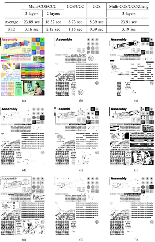
C. Computation Time
Table IV shows the computation time in seconds for multi-scale-COS/CCC with three layers, multimulti-scale-COS/CCC with two layers, COS/CCC, COS, and multiscale-COS/CCC/Zheng. We evaluated the computation time using an Intel Xeon CPU (3.20 GHz), and the numbers are averaged on 21 test images. The block size on the finest resolution layer is set to 32. No-tice that the computation time of multiscale segmentation grows almost linearly as the number of layers increases. The compu-tation time of our multiscale-COS/CCC and multiscale-COS/ CCC/Zheng are almost same. We also found that the computa-tion time for Otsu and Tsai thresholding methods are 0.02 sec-onds for all of the test images.
D. Qualitative Results
Fig. 10 illustrates segmentations generated by Otsu/CCC, multiscale-COS/CCC/Zheng, DjVu, LuraDocument, COS, COS/CCC, and multiscale-COS/CCC for a 300 dpi test image. The ground truth segmentation is also shown. This test image contains many complex features such as different color text, light-color text on a dark background, and various sizes of text. As it is shown, COS accurately detects most text components but the number of false detections is quite large. However, COS/CCC eliminates most of these false detections without
significantly sacrificing text detection. In addition, multi-scale-COS/CCC generally detects both large and small text with minimal false component detection. Otsu/CCC method misses many text detections. LuraDocument is very sensitive to sharp edges embedded in picture regions and detects a large number of false components. DjVu also detects some false components but the error is less severe than LuraDocument. Multiscale-COS/CCC/Zheng’s result is similar to our multi-scale-COS/CCC result but our text detection error is slightly less.
Figs. 11 and 12 show a close up of text regions and picture regions from the same test image. In the text regions, our al-gorithms (COS, COS/CCC, and multiscale-COS/CCC), multi-scale-COS/CCC/Zheng, and Otsu/CCC provided detailed text detection while DjVu and LuraDocument missed sections of these text components. In the picture regions, while our COS algorithm contains many false detections, COS/CCC and mul-tiscale-COS/CCC algorithms are much less susceptible to these false detections. The false detections by COS/CCC and multi-scale-COS/CCC are also less than DjVu, LuraDocument, and multiscale-COS/CCC/Zheng.
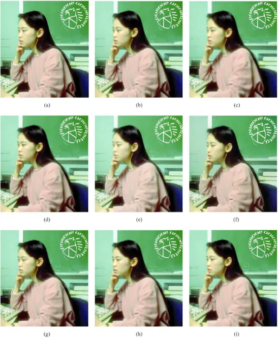
Figs. 13 and 14 show MRC decoded images when the en-codings relied on segmentations from Ground truth, Otsu/CCC, multiscale-COS/CCC/Zheng, DjVu, LuraDocument, COS, COS/CCC, and multiscale-COS/CCC. The examples from text and picture regions illustrate how segmentation accuracy affects the decoded image quality. Note that the MRC encoding method used after segmentation is different for each package, and MRC encoders used in DjVu and LuraDocument are not open source, therefore we developed our own MRC encoding scheme. This comparison is not strictly limited to segmentation effects, but it provides an illustration of how missed components and false component detection affects the decoded images.
As shown in Fig. 13, all of the text from COS, COS/CCC, multiscale-COS/CCC, and multiscale-COS/CCC/Zheng is
Fig. 12. Picture regions in the binary mask. Picture region is 151621003 pixels at 400 dpi, which corresponds to 9.63 cm26.35 cm. (a) Original test image. (b) Ground truth segmentation. (c) Otsu/CCC. (d) Multiscale-COS/CCC/Zheng. (e) DjVu. (f) LuraDocument. (g) COS. (h) COS/CCC. (i) Multiscale-COS/CCC.
Fig. 13. Decoded MRC image of text regions (400 dpi). (a) Original test image. (b) Ground truth (300:1 compression). (c) Otsu/CCC (311:1 compression). (d) Multiscale-COS/CCC/Zheng (295:1). (e) DjVu (281:1). (f) LuraDocument (242:1). (g) COS (244:1). (h) COS/CCC (300:1). (i) Multiscale-COS/CCC (289:1).
clearly represented. Some text in the decoded images from Otsu/CCC, DjVu, and LuraDocument are blurred because missed detection placed these components in the background. In the picture region, our methods classify most of the parts as background so there is little visible distortion due to mis-seg-mentation. On the other hand, the falsely detected components in DjVu and LuraDocument generate artifacts in the decoded
images. This is because the text-detected regions are repre-sented in the foreground layer, therefore the image in those locations is encoded at a much lower spatial resolution. E. Prior Model Evaluation
In this section, we will evaluate our selected prior model. We used the initial segmentation result generated by COS with
Fig. 14. Decoded MRC image of picture regions (400 dpi). (a) Original test image. (b) Ground truth (300:1 compression). (c) Otsu/CCC (311:1 compression). (d) Multiscale-COS/CCC/Zheng (295:1). (e) DjVu (281:1). (f) LuraDocument (242:1). (g) COS (244:1). (h) COS/CCC (300:1). (i) Multiscale-COS/CCC (289:1).
a single block size 32 32. Then we performed the CCC seg-mentation with the same parameter set described in the pre-vious section. Fig. 15 shows the local conditional probability of each connected component given its neighbors’ classes for two test images. The colored components indicate the foreground regions segmented by the COS algorithm. The yellowish or re-dish components were classified as text by the CCC algorithm, whereas the bluish components were classified as nontext. The brightness of each connected component indicates the intensity of the conditional probability which is described as . As shown, the conditional probability of assigned classifica-tion are close to 1 for most components. We observed that the components on boundaries between text and nontext regions take slightly smaller values but overall this local conditional probability map shows that the contextual model fits the test
data well, and that the prior term contributes to an accurate classification.
VI. CONCLUSION
We presented a novel segmentation algorithm for the compression of raster documents. While the COS algorithm generates consistent initial segmentations, the CCC algorithm substantially reduces false detections through the use of a component-wise MRF context model. The MRF model uses a pair-wise Gibbs distribution which more heavily weights nearby components with similar features. We showed that the multiscale-COS/CCC algorithm achieves greater text detection accuracy with a lower false detection rate, as compared to state-of-the-art commercial MRC products. Such text-only seg-mentations are also potentially useful for document processing applications such as OCR.
Fig. 15. Yellowish or redish components were classified as text by the CCC algorithm, whereas the bluish components were classified as nontext. The brightness of each connected component indicates the intensity of the conditional probability which is described asP (x jx ). (a) Original training image. (b) Local proba-bilities. (c) Original test image. (d) Local probaproba-bilities.
APPENDIX
FEATUREVECTOR FORCCC
The feature vector for the connected components ex-tracted in the CCC algorithm is a 4-D vector and denoted as . Two of the components describe edge depth information, while the other two describe pixel value uniformity.
More specifically, an inner pixel and an outer pixel are first defined to be the two neighboring pixels across the
boundary for each boundary segment ,
where is the length of the boundary. Note that the inner pixel is a foreground pixel and the outer pixel is a background pixel. The inner pixel values are defined as , whereas the outer pixel
values are defined as .
Using these definitions, the edge depth is defined as
Then, the terms and are defined as Sample mean of edge
Standard deviation of edge
The terms and describe uniformity of the outer pixels. The uniformity is defined by the range and standard deviation of the outer pixel values, that is
Standard deviation of where
In an actual calculation, the 95th percentile and the fifth per-centile are used instead of the maximum and minimum values to eliminate outliers. Note that only outer pixel values were examined for the uniformness because we found that inner
pixel values of the connected components extracted by COS are mostly uniform even for nontext components.
The augmented feature vector of CCC algorithm contains the four components described previously concatenated with two additional components corresponding the horizontal and ver-tical position of the connected component’s center in 300 dpi,
that is .
horizontal pixel location of a connected component's center
vertical pixel location of a connected component's center
ACKNOWLEDGMENT
The authors would like to thank S. H. Kim and J. Yi at Samsung Electronics for their support of this research.
REFERENCES
[1] ITU-T Recommendation T.44 Mixed Raster Content (MRC), T.44, In-ternational Telecommunication Union, 1999.
[2] G. Nagy, S. Seth, and M. Viswanathan, “A prototype document image analysis system for technical journals,”Computer, vol. 25, no. 7, pp. 10–22, 1992.
[3] K. Y. Wong and F. M. Wahl, “Document analysis system,”IBM J. Res. Develop., vol. 26, pp. 647–656, 1982.
[4] J. Fisher, “A rule-based system for document image segmentation,” in
Proc. 10th Int. Conf. Pattern Recognit., 1990, pp. 567–572.
[5] L. O’Gorman, “The document spectrum for page layout anal-ysis,”IEEE Trans. Pattern Anal. Mach. Intell., vol. 15, no. 11, pp. 1162–1173, Nov. 1993.
[6] Y. Chen and B. Wu, “A multi-plane approach for text segmentation of complex document images,”Pattern Recognit., vol. 42, no. 7, pp. 1419–1444, 2009.
[7] R. C. Gonzalez and R. E. Woods, Digital Image Processing, 3rd ed. Upper Saddle River, NJ: Pearson Education, 2008.
[8] F. Shafait, D. Keysers, and T. Breuel, “Performance evaluation and benchmarking of six-page segmentation algorithms,”IEEE Trans. Pat-tern Anal. Mach. Intell., vol. 30, no. 6, pp. 941–954, Jun. 2008. [9] K. Jung, K. Kim, and A. K. Jain, “Text information extraction in images
and video: A survey,”Pattern Recognit., vol. 37, no. 5, pp. 977–997, 2004.
[10] G. Nagy, “Twenty years of document image analysis in PAMI,”IEEE Trans. Pattern Anal. Mach. Intell., vol. 22, no. 1, pp. 38–62, Jan. 2000. [11] A. K. Jain and B. Yu, “Document representation and its application to page decomposition,”IEEE Trans. Pattern Anal. Mach. Intell., vol. 20, no. 3, pp. 294–308, Mar. 1998.
[12] N. Otsu, “A threshold selection method from gray-level histograms,”
IEEE Trans. Syst., Man Cybern., vol. 9, no. 1, pp. 62–66, Jan. 1979. [13] H. Oh, K. Lim, and S. Chien, “An improved binarization algorithm
based on a water flow model for document image with inhomogeneous backgrounds,”Pattern Recognit., vol. 38, no. 12, pp. 2612–2625, 2005. [14] W. Niblack, An Introduction to Digital Image Processing. Upper
Saddle River, NJ: Prentice-Hall, 1986.
[15] J. Sauvola and M. Pietaksinen, “Adaptive document image binariza-tion,”Pattern Recognit., vol. 33, no. 2, pp. 236–335, 2000.
[16] J. Kapur, P. Sahoo, and A. Wong, “A new method for gray-level picture thresholding using the entropy of the histogram,”Graph. Models Image Process., vol. 29, no. 3, pp. 273–285, 1985.
[17] W. Tsai, “Moment-preserving thresholding: A new approach,”Graph. Models Image Process., vol. 29, no. 3, pp. 377–393, 1985.
[18] P. Stathis, E. Kavallieratou, and N. Papamarkos, “An evaluation survey of binarization algorithms on historical documents,” inProc. 19th Int. Conf. Pattern Recognit., 2008, pp. 1–4.
[19] J. M. White and G. D. Rohrer, “Image thresholding for optical char-acter recognition and other applications requiring charchar-acter image ex-traction,”IBM J. Res. Develop., vol. 27, pp. 400–411, 1983.
[20] M. Kamel and A. Zhao, “Binary character/graphics image extraction: A new technique and six evaluation aspects,” inProc. IAPR Int. Conf., 1992, vol. 3, pp. 113–116.
[21] Y. Liu and S. Srihari, “Document image binarization based on texture features,”IEEE Trans. Pattern Anal. Mach. Intell., vol. 19, no. 5, pp. 540–544, May 1997.
[22] C. Jung and Q. Liu, “A new approach for text segmentation using a stroke filter,”Signal Process., vol. 88, no. 7, pp. 1907–1916, 2008. [23] R. de Queiroz, Z. Fan, and T. Tran, “Optimizing block-thresholding
segmentation for multilayer compression of compound images,”IEEE Trans. Image Process., vol. 9, no. 9, pp. 1461–1471, Sep. 2000. [24] H. Cheng and C. A. Bouman, “Document compression using
rate-dis-tortion optimized segmentation,”J. Electron. Imag., vol. 10, no. 2, pp. 460–474, 2001.
[25] L. Bottou, P. Haffner, P. G. Howard, P. Simard, Y. Bengio, and Y. LeCun, “High quality document image compression with DjVu,”J. Electron. Imag., vol. 7, no. 3, pp. 410–425, 1998.
[26] P. Haffner, L. Bottou, and Y. Lecun, “A general segmentation scheme for DjVu document compression,” inProc. ISMM, Sydney, Australia, Apr. 2002, pp. 17–36.
[27] Luradocument Pdf Compressor [Online]. Available: https://www.lu-ratech.com
[28] Y. Zheng and D. Doermann, “Machine printed text and handwriting identification in noisy document images,”IEEE Trans. Pattern Anal. Mach. Intell., vol. 26, no. 3, pp. 337–353, Mar. 2004.
[29] S. Kumar, R. Gupta, N. Khanna, S. Chaundhury, and S. D. Joshi, “Text extraction and document image segmentation using matched wavelets and MRF model,”IEEE Trans. Image Process., vol. 16, no. 8, pp. 2117–2128, Aug. 2007.
[30] J. Kuk, N. Cho, and K. Lee, “MAP-MRF approach for binarization of degraded document image,” inProc. IEEE Int. Conf. Image Process., 2008, pp. 2612–2615.
[31] H. Cao and V. Govindaraju, “Processing of low-quality handwritten documents using Markov random field,”IEEE Trans. Pattern Anal. Mach. Intell., vol. 31, no. 7, pp. 1184–1194, Jul. 2009.
[32] J. Lafferty, A. McCallum, and F. Pereira, “Conditional random fields: Probabilistic models for segmenting and labeling sequence data,” in
Proc. 18th Int. Conf. Mach. Learn., 2001, pp. 282–289.
[33] S. Kumar and M. Hebert, “Discriminative random fields: A discrimi-native framework for contextual interaction in classification,” inProc. Int. Conf. Comput. Vis., 2003, vol. 2, pp. 1150–1157.
[34] M. C.-P. A. X. He and R. S. Zemel, “Multiscale conditional random fields for image labeling,” inProc. IEEE Comput. Soc. Conf. Comput. Vis. Pattern Recognit., 2004, vol. 2, pp. 695–702.
[35] M. Li, M. Bai, C. Wang, and B. Xiao, “Conditional random field for text segmentation from images with complex background,”Pattern Recognit. Lett., vol. 31, no. 14, pp. 2295–2308, 2010.
[36] E. Haneda, J. Yi, and C. A. Bouman, “Segmentation for MRC com-pression,” inProc. Color Imag. XII, San Jose, CA, Jan. 29, 2007, vol. 649304, pp. 1–12.
[37] T. H. Cormen, C. E. Leiserson, R. L. Rivest, and C. Stein, Introduction to Algorithms, 2nd ed. New York: McGraw-Hill, 2001.
[38] J. Besag, “On the statistical analysis of dirty pictures,”J. Roy. Statist. Soc. B, vol. 48, no. 3, pp. 259–302, 1986.
[39] C. A. Bouman, Digital Image Processing Laboratory: Markov Random Fields and MAP Image Segmentation 2007 [Online]. Available: http:// www.ece.purdue.edu/~bouman
[40] C. A. Bouman, Cluster: An Unsupervised Algorithm for Modeling Gaussian Mixtures 1997 [Online]. Available: http://www.ece.purdue. edu/~bouman
[41] J. Rissanen, “A universal prior for integers and estimation by minimum description length,”Ann. Statist., vol. 11, no. 2, pp. 417–431, 1983. [42] J. Besag, “Spatial interaction and the statistical analysis of lattice
sys-tems,”J. Roy. Statist. Soc. B, vol. 36, no. 2, pp. 192–236, 1974. [43] J. Besag, “Statistical analysis of non-lattice data,”Statistician, vol. 24,
no. 3, pp. 179–195, 1975.
[44] J. Besag, “Efficiency of pseudolikelihood estimation for simple Gaussian fields,”Biometrika, vol. 64, no. 3, pp. 616–618, 1977. [45] C. A. Bouman and B. Liu, “Multiple resolution segmentation of
Tex-tured images,”IEEE Trans. Pattern Anal. Mach. Intell., vol. 13, no. 2, pp. 99–113, Feb. 1991.
[46] C. A. Bouman and M. Shapiro, “A multiscale random field model for Bayesian image segmentation,”IEEE Trans. Image Process., vol. 3, no. 2, pp. 162–177, Feb. 1994.
[47] H. Cheng and C. A. Bouman, “Multiscale Bayesian segmentation using a trainable context model,”IEEE Trans. Image Process., vol. 10, no. 4, pp. 511–525, Apr. 2001.
[48] Document Express With DjVu [Online]. Available: https://www. celartem.com
[49] IEC 61966-2-1. : Int. Electrotech. Commission, 1999 [Online]. Available: http://www.iec.ch
[50] H. Siddiqui and C. A. Bouman, “Training-dased descreening,”IEEE Trans. Image Process., vol. 16, no. 3, pp. 789–802, Mar. 2007. [51] A. Osman, Z. Pizlo, and J. Allebach, “CRT calibration techniques for
better accuracy including low luminance colors,” inProc. SPIE Conf. Color Imag., San Jose, CA, Jan. 2004, vol. 5293, pp. 286–297. [52] ITU-T Recommendation T.88 Lossy/Lossless Coding of Bi-Level
Images. : Int. Telecommun. Union, 2000 [Online]. Available: http://www.itu.int/ITU-T
[53] P. G. Howard, F. Kossentini, B. Martins, S. Forchhammer, W. J. Ruck-lidge, and F. Ono, The Emerging JBIG2 Standard [Online]. Available: citeseer.ist.psu.edu/howard98emerging.html
Eri Haneda (S’10) received the B.S. degree in electrical engineering from Tokyo Institute of Technology, Japan, in 1997, the M.S. degree from Purdue University, West Lafayette, IN, in 2003, and is currently pursuing the Ph.D. degree in the School of Electrical and Computer Engineering, Purdue University.
From 1997 to 2000, she worked for the Switching & Mobile Communication Department, NEC Com-pany Ltd., Japan. Her research interests are in statis-tical image processing such as image segmentation, image restoration, and medical imaging.
Charles A. Bouman (S’86–M’89–SM’97–F’01) received the B.S.E.E. degree from the University of Pennsylvania, Philadelphia, in 1981, the M.S. degree from the University of California, Berkeley, in 1982, and the Ph.D. degree in electrical engineering from Princeton University, Princeton, NJ, in 1989.
From 1982 to 1985, he was a full staff member at the Massachusetts Institute of Technology Lin-coln Laboratory. In 1989, he joined the faculty of Purdue University, West Lafayette, IN, where he is a Professor with a primary appointment in the School of Electrical and Computer Engineering and a secondary appointment in the School of Biomedical Engineering. Currently, he is Co-Director of Purdue’s Magnetic Resonance Imaging Facility located in Purdue’s Research Park. His research focuses on the use of statistical image models, multiscale techniques, and fast algorithms in applications including tomographic reconstruction, medical imaging, and document rendering and acquisition.
Prof. Bouman is a Fellow of the IEEE, a Fellow of the American Institute for Medical and Biological Engineering (AIMBE), a Fellow of the society for Imaging Science and Technology (IS&T), a Fellow of the SPIE professional society, a recipient of IS&T’s Raymond C. Bowman Award for outstanding contributions to digital imaging education and research, and a University Fac-ulty Scholar of Purdue University. He was the Editor-in-Chief of the IEEE TRANSACTIONS ONIMAGEPROCESSINGand a member of the IEEE Biomedical Image and Signal Processing Technical Committee. He has been a member of the Steering Committee for the IEEE TRANSACTIONS ONMEDICALIMAGINGand an Associate Editor for the IEEE TRANSACTIONS ONIMAGEPROCESSINGand the IEEE TRANSACTIONS ONPATTERNANALYSIS ANDMACHINEINTELLIGENCE. He has also been Co-Chair of the 2006 SPIE/IS&T Symposium on Electronic Imaging, Co-Chair of the SPIE/IS&T Conferences on Visual Communications and Image Processing 2000 (VCIP), a Vice President of Publications and a member of the Board of Directors for the IS&T Society, and he is the founder and Co-Chair of the SPIE/IS&T Conference on Computational Imaging.