UNIVERSIDAD AUTÓNOMA DE MADRID
ESCUELA POLITÉCNICA SUPERIOR
Double Degree in Computer Science and Mathematics
DEGREE WORK
Development of a Python package for Functional
Data Analysis
Depth Measures, Applications and Clustering
Author: Amanda Hernando Bernabé
Advisor: José Luis Torrecilla
© 3 de Noviembre de 2017 by UNIVERSIDAD AUTÓNOMA DE MADRID Francisco Tomás y Valiente, no1
Madrid, 28049 Spain
Amanda Hernando Bernabé
Development of a Python package for Functional Data Analysis
Amanda Hernando Bernabé
C\ Francisco Tomás y Valiente Nº 11
A mi familia y a mis amigos
Striving for success without hard work is like trying to harvest where you haven’t planted.
A
gradecimientos
Me gustaría dar las gracias a todo el equipo que forma parte de este proyecto. A Alberto Suárez por proponerlo y darme la oportunidad de participar en una iniciativa con aplicación en el mundo real a corto plazo. A José Luis Torrecilla por introducirme en la parte más teórica de los datos funcionales y a Carlos Ramos por el gran esfuerzo hecho enseñándome Python. Además agradezco a mis compañe-ros Pablo Pérez y Pablo Marcos la facilidad de trabajar con ellos y la motivación puesta en el proyecto. Por último, agradecer a Eloy Anguiano la plantilla de este artículo que ha hecho la escritura mucho menos tediosa.
R
esumen
En este trabajo, se aborda el problema del Análisis de Datos Funcionales (FDA). Cada observación en datos funcionales es una función que varía sobre un continuo. Este tipo de datos complejos se está volviendo cada vez más común en muchos campos de la investigación. Sin embargo, el Análisis de Datos Funcionales es un campo relativamente reciente en el que las implementaciones de software se limitan básicamente a R. Además, aunque siguan un esquemaopen-source, la contibución a las mis-mas puede resultar dificultosa. El objetivo final de este proyecto es proporcionar un paquete completo,
scikit-fda, para el Análisis de Datos Funcionales escrito en Python.
En este trabajo de fin de grado, la funcionalidad implementada en el paquete incluye las medidas de profundidad funcional junto con sus aplicaciones y nociones elementales de clustering. En los espacios funcionales, establecer un orden es complicado debido a su naturaleza. Las medidas de profundidad permiten definir estadísticos robustos para los datos funcionales. En el paquete se pueden encontrar unas de las más habituales, la medida de profundidad de Fraiman y Muñiz, la band depth o una modificación de esta última, la modified band depth. Las medidas de profundidad se utilizan en la construcción de herramientas gráficas, tanto el diagrama de caja funcional como elmagnitude-shape plot se introducen en el paquete además de sus procedimientos de detección de valores atípicos. Asimismo, se realizan contribuciones en el área del aprendizaje automático en el cual se añaden algoritmos básicos de clustering al paquete: K-means y Fuzzy K-means. Finalmente, se muestran los resultados de la aplicación de estos métodos al conjunto de datos del clima canadiense.
El paquete Python está publicado en un repositorio de GitHub. Esopen-sourcecon el objetivo de crecer y mantenerse actualizado. A largo plazo, se espera que cubra las técnicas fundamentales del FDA y se convierta en unatoolboxampliamente utilizada para la investigación en el FDA.
P
alabras clave
Análisis de Datos Funcionales, Medidas de Profundidad, Diagrama de Caja, Detección de datos atípicos, Clustering, Python, Software
A
bstract
In this paper, the problem of analyzing functional data is addressed. Each observation in functional data is a function that varies over a continuum. This kind of complex data is increasingly becoming more common in many research fields. However, Functional Data Analysis (FDA) is a relatively recent field in which software implementations are basically limited to R. In addition, although they may follow an open-source scheme, the contribution to them may turn out to be complicated. The final goal of this project is to provide a comprehensive Python package for Functional Data Analysis,scikit-fda.
In this undergraduate thesis, the functionality implemented in the package includes functional depth measures together with their applications and elementary notions of clustering. In a functional space, establishing an order is complicated due to its nature. Depth measures allow to define robust statistics for functional data. In the package you can find some of the most common, Fraiman and Muniz depth measure, the band depth measure or a modification of the latter, the modified band depth. Depth mea-sures are used in the construction of graphic tools, both the functional boxplot and the magnitude-shape plot are introduced in the package along with their outlier detection procedures. Furthermore, contribu-tions in the area of machine learning are made in which basic clustering algorithms are added to the package: K-means and Fuzzy K-means. Finally, the results of applying these methods to the Canadian Weather dataset are shown.
The Python package is published in a GitHub repository. It is open-source wth the aim of growing and being kept up to date. In the long term it is expected to cover the fundamental techniques in FDA and become a widely-used toolbox for research in FDA.
K
eywords
Functional Data Analysis, Depth Measures, Boxplot, Outlier detection, Clustering, Python, Software
T
able of
C
ontents
1 Introduction 1
1.1 Goals and Scope . . . 1
1.2 Document Structure . . . 2
2 State of the Art - FDA: Depth Measures, Applications and Clustering 3 2.1 Functional Depth . . . 5
2.1.1 Fraiman and Muniz Depth . . . 7
2.1.2 Band Depth and Modified Band Depth . . . 8
2.2 Functional Boxplot . . . 10
2.3 Magnitude-Shape Plot . . . 12
2.4 Clustering Algorithms . . . 15
2.4.1 K-means . . . 16
2.4.2 Fuzzy K-means . . . 17
3 Software Development Process 19 3.1 Analysis . . . 19
3.2 Design . . . 20
3.3 Coding, Documentation and Testing . . . 23
3.4 Version Control and Continuous Integration . . . 24
4 Results 27
5 Future Work and Conclusions 33
Bibliography 36
Appendices
37
A Documentation 39
L
ists
List of algorithms
2.1 K-means algorithm.. . . 17
2.2 Fuzzy K-means algorithm.. . . 18
3.1 Band Depth pseudocode. . . 21
3.2 Modified Band Depth pseudocode.. . . 21
List of equations
2.1 Multivariate point-type data depth function. . . 52.2 Functional depth function in terms of multivariate point-type data depth. . . 6
2.3 Development of the multivariate functional depth function in terms of univariate depth. 6 2.4 Multivariate functional depth function based on univariate depth function. . . 7
2.5 FM cumulative distribution function. . . 7
2.6 Univariate Fraiman and Muniz depth function . . . 7
2.7 Multivariate functional Fraiman and Muniz depth function . . . 8
2.8 Band defined by several curves. . . 8
2.9 Proportion of bands containing a specific curve . . . 8
2.10 Univariate functional band depth. . . 8
2.11 Multivariate functional band depth. . . 9
2.12 Proportion of time a curve is contained in the bands . . . 9
2.13 Functional boxplot central region definition . . . 10
2.14 Functional outlyingess. . . 12
2.15 Functional directional outlyingess . . . 13
2.16 Mean directional outlyingess . . . 13
2.17 Variation directional outlyingess. . . 13
2.18 Functional directional outlyingess . . . 13
2.19 Descompotition of the functional directional outlyingess . . . 14
2.20 Discrete mean directional outlyingess. . . 14
2.21 Square robust Mahalanobis distance ofYk,n . . . 15
2.22 K-means minimization function . . . 16
2.23 Fuzzy K-means minimization function. . . 17
2.2 Canadian Weather dataset . . . 4
2.3 FM depth in terms of the distribution . . . 7
2.4 Introductory example of BD and MBD . . . 9
2.5 Example boxplot . . . 11
2.6 Example enhanced boxplot . . . 11
2.7 Example surface boxplot . . . 12
2.8 Introductory magnitude-shape plot. . . 14
3.1 Functionality map of scikit-fda. . . 20
3.2 Git flow . . . 24
4.1 Complete Canadian Weather dataset . . . 27
4.2 Boxplot of the Canadian temperatures. . . 28
4.3 Enhanced boxplot of the Canadian temperatures . . . 28
4.4 MS-plot of the Canadian temperatures-MBD . . . 29
4.5 MS-plot groupings of the Canadian temperatures-FM. . . 29
4.6 MS-plot groupings of the Canadian temperatures-MBD . . . 30
4.7 Clustering plot of the Canadian temperatures. . . 30
4.8 Clustering lines plot of the Canadian temperatures . . . 31
4.9 Clustering bars plot of the Canadian temperatures . . . 31
1
I
ntroduction
In recent years, Functional Data Analysis (FDA) has become one of the most active domains in Statistics. The objects under study are real functions which are assumed to be realizations of stochastic processes that can represent curves, surfaces or anything else varying over a continuum.
Due to the advances in technology, such functional data can be collected in many scientific areas including but not limited to biology, finance, engineering, medicine and meteorology. As a result, FDA has engaged an increasing number of researchers during the past decades. Many methods have been proposed to extract useful information from functional data. The main references in this field are Ramsay and Silverman (2005) [1], and Ferraty and Vieu (2006) [2].
Nevertheless, software implementations are restricted fundamentally to R programming language. The available packages include some general purpose ones, such asfda[3] orfda.usc [4] and others more specific, among which the refund [5], roahd [6] or rainbow [7] packages can be found. They implement functionality regarding regression, robust statistics and visualization techniques respectively. All of them can be found in the The Comprehensive R Archive Network (CRAN) repository. More rare to encounter, there are also implementations written in Matlab. They include also thefda[3] package or the PACE [8] package, the latter developed by the Department of Statistics at the University of California. As a consequence, the implementation of a Python package for FDA was considered to be a valua-ble tool for the increasing number of researchers who are adopting this language. In addition, dealing with an open-source software in which continuous collaboration is possible promotes an up-to-date tool.
1.1.
Goals and Scope
The main purpose of this project is to expand the functionality ofscikit-fda, the Python FDA package started last year by the former student Miguel Carbajo [9]. The initial version of the package contained some basic tools to work with functional data. The functionality implemented was principally related with the representation of the objects studied: functions.
The functions are commonly assumed to belong to a Hilbert space and to be able to be represented with a convenient functional basis, such as B-Splines or Fourier. On the other hand, individual observa-tions are generally recorded only in a finite number of moments, giving rise to a grid. As a consequence, we often work with discretized versions of the functional data. These two frameworks were addressed in scikit-fda by means of two classes: FDataGrid and FDataBasis respectively. They included methods to compute the basic statistics and to change from one representation to another. Furthermore, simple smoothing techniques were also covered.
From this base, the functionality implemented includes depth measures along with their applications and some fundamental methods for clustering functional data. Due to the complexity of functional spa-ces, they do not present a natural order such as the one found in the real line. An approach proposed to cover this lack of a definition of distance between functions resides in the idea of functional depth. Functional depth introduces an ordering within a sample and can provide a measure to analyze how similar observations are. Functional depth measures implemented include Fraiman and Muniz depth, the band depth and the modified band depth.
Having ranks of curves, the functional boxplot, an appealing visualization tool, is implemented as a natural extension of the classical boxplot. Another graphical tool for visualizing centrality and detec-ting outliers for functional data, the magnitude-shape plot, has been included. Moreover, once specific distances are defined, clustering algorithms can be applied straightforward to the data. Both K-means and Fuzzy K-means algorithms can be found in the package. The results can be plotted as an effective way to illustrate the characteristics that are not apparent from the mathematical models or summary statistics.
1.2.
Document Structure
The paper is organized as follows. In Chapter 2, Functional Data Analysis is introduced. A brief overview is given followed by a deeper presentation of functional depth, its applications and clustering analysis in functional data. Each of the tools implemented is discussed in detail, both the practical context and theoretic calculations are explained. In Chapter3, the solution implemented is described, which can be object oriented or consist in a functional approach. The possible customizations of the classes or methods are also exposed. The results obtained applying the functionality introduced to the package are shown in Chapter 4. In order to do this, a specific dataset is chosen and the different methods are applied to it: the boxplot, the magnitude-shape plot and the clustering algorithms. Chapter 5 contains the future work and conclusions. Finally, Appendix A contains the documentation found online forscikit-fda. First, the practical examples found in Jupyter Notebooks are appended and then, the documentation of the classes and functions implemented.
2
S
tate of the
A
rt
- FDA: D
epth
M
easures
, A
pplications and
C
lustering
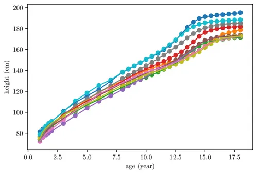
Nowadays, data are frequently obtained as trajectories or images in many research fields. Typically, a functional dataset consists ofncurves measured at different time points,Tk={t1, t2, ..., tk}, which do not need to be equally spaced. In the example below2.1, obtained from the Berkeley Growth Study [3], we can observe the heights of 10 children measured at a set of 31 ages, between 1 and 18 years old. The observations are recorded every 3 months during the first year, every year until the age of 8, and during the next ten years every half a year.
0.0 2.5 5.0 7.5 10.0 12.5 15.0 17.5 age (year) 80 100 120 140 160 180 200 heigh t (cm)
Berkeley Growth Study
Figure 2.1:The heights of 10 children measured at 31 ages. The circles indicate the unequally spaced 31 measurements of each boy or girl.
Interesting questions that could be asked include, how much a child grow on average, at what age children have a more equally height, is this child abnormally tall/short (which can derive in a growing problem) or does this observation belong to a girl or a boy. This questions are related to the estimation of the central tendency of the curves, to the estimation of the variability among the curves, the detection of outlying curves, and the classification of such curves respectively.
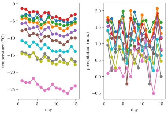
Multivariate functional data are also considered along the paper. Each multivariate functional datum consists of a set ofdcurves. In this context, the Canadian Weather dataset [3] can be mentioned since it contains simultaneous observations of temperature and precipitation measurements (d = 2) recor-ded every day during a year in different Canadian weather stations. Only the measurements recorrecor-ded in ten weather stations the first two weeks of the year are shown in Figure2.2in order to observe the equally spaced time points. Additionally, spatial surfaces can be considered, in which now the multi-ple dimensions are found on the domain. Exammulti-ples include face recognition or neurological disorders assessment with brain images. These last ones can be found in [10].
0 5 10 15 day −25 −20 −15 −10 −5 0 temp erature ( º C) 0 5 10 15 day −0.5 0.0 0.5 1.0 1.5 2.0 precipitation (mm.)
Canadian Weather
Figure 2.2:The temperatures and precipitations recorded in 10 different weather stations every day during a year. Only the fisrt 15 days of the year are plotted to show the equally spaced design points.
Notation
Before going into detail, let specify some notation. Consider a q-variate stochastic process X = (X1, X2, ..., Xq)T : I −→ Rq where the coordinates Xi : I −→ R, for 1 ≤ i ≤ q, are univariate
stochastic processes. In most cases, I is a compact interval which belongs to R. Nevertheless, this
definition changes for multiple dimensions on the domain,I should be a compact set defined on the domain space ofX. For example, in a brain image the domain belongs to R2, so the compact set is the cross-section area of the brain. Besides, q, a positive integer, indicates the dimensionality of the functional data. Ifq = 1, univariate functional data are considered, as in the example of the Berkeley Growth Study, whereas ifq ≥ 2, multivariate functional data are found, as in the Canadian Weather dataset.Xtakes values in the spaceC(I,Rq)of real continuous functions with probability distribution
2.1. FunctionalDepth
FX.
Furthermore, a stochastic process can be seen as a family of random variables. At each design pointt ∈ I, X(t) is aq-variate random variable, or random vector, with probability distributionFX(t).
Along the document, the random variables are indexed by the setTk ⊂I. In the weather example, the 2-dimensional random vector of each day is composed of the temperature and precipitation measure-ments. IfI is multidimensional,X(t)is called random field.
Additionally, for a sample of independent and identically distributed stochastic processesX1,X2, ...,Xn, the empirical distribution is denoted withFX,n. Analogously,FX(t),n is used for the random variables
X1(t),X2(t), ...,Xn(t).
2.1.
Functional Depth
Statistical depth provides a measure of centrality or outlyingness of an observation with respect to a given dataset or population distribution. The most central object is assigned the highest value while the least central, the lowest value. Those values are positive and bounded, without loss of generality, the explanation is given with the interval [0,1] ⊂ R. Since in functional spaces there is no natural
order, depths, which provide rankings of curves and a notion of centrality, are very useful. The uses of statistical depths include the construction of linear estimators, or functional boxplots, the detection of outlying observations or the classification of the data among others.
Although depth measures in R are trivial, this is not the case in the multivariate setting nor the
functional. First, for each t ∈ Tk, consider the one dimensional random variable X(t) and a depth measure denoted byd X(t), FX(t)
:X(t) −→ [0,1]. In this case, there are no doubts of the order independently of the metric considered. The properties are clear in R and the deepest observation is the median. One approach of extending this definition to the multivariate setting is to regard the depth value of a random vector as a weighted average of the marginal depths. As a consequence, the statistical depth measured X(t), FX(t)
: X(t) −→ [0,1] for a multivariate random vector X(t) is calculated as: d X(t), FX(t) = q X i=1 d Xi(t), FXi(t) ·pi, q X i=1 pi = 1, (2.1)
wherepi, for1 ≤ i ≤ q are the weights given to each of the dimensions. As a result, the multi-variate depths are used to rank the marginal observations of a sample of multimulti-variate functional data
X1(t),X2(t), ...,Xn(t)found at each design point.
Noteworthy contributions proposed to rank multivariate data include the halfspace depth by Tukey (1975) [11] or the simplicial depth by Liu (1990) [12] and Zuo and Serfling (2000) [13] introduced the
key properties that a depth function should verify: affine invariance, maximality at center, monotonicity and vanishing at infinity.
Finally, we still need to order functions over time. This is a much more difficult problem since, as a difference with respect toRq, in a functional space distinct metrics are no longer equivalent. This leads
to very different rankings depending on the depth measure.
A first attempt to extend the previous definitions to the functional setting are the so-called integral depths, based on the integration of the marginal depths (univariate or multivariate) over time. Hence, for a stochastic processX, an integral depth function is:
d(X, FX) = Z I d X(t), FX(t)·w(t)dt, Z I w(t) = 1, (2.2)
wherew(t) is a weight function defined onI. Usually,w(t) = {λ(I)}−1 being λ(·)the Lebesgue measure.
Replacing the multivariate pointwise depth with Equation2.1: d(X, FX) = Z I d X(t), FX(t) ·w(t)dt = Z I q X i=1 d Xi(t), FXi(t) ·pi ! ·w(t)dt = q X i=1 Z I d(Xi(t), FXi(t))·w(t)dt ·pi = q X i=1 d(Xi, FXi)·pi, (2.3)
another definition for a multivariate stochastic process depth function is obtained in terms of the univariate processes.
The numerous notions of depth encountered in the literature vary regarding robustness, sensitivity to reflect asymmetric shapes or computability. In any case, all of them allow to sort a sample of functional dataX1,X2, ...,Xnaccording to their depth obtaining the order statisticsX(1),X(2), ...,X(n). If curves are sorted by their decreasing depth, the median (based on this depth) can be defined as the deepest point,X(1). While the median is the observations that stays morein the middle of the set and has the
highest depth value, the curves further away from the rest, with depth values proximate to zero, can be considered as theouter skinof the data and sometimes outliers.
The functional depths implemented in the package include Fraiman and Muniz, Band Depth and a modification of this last one, the Modified Band Depth. The first one is explained following the first approach2.2while the others, the second approach (inferred from2.3) based in a weighted average of
2.1. FunctionalDepth
the univariate stochastic processes:
d(X, FX) =
q X
i=1
d(Xi, FXi)∗pi. (2.4)
2.1.1.
Fraiman and Muniz Depth
Fraiman and Muniz (FM) [14] proposed the first integral depth for functional data. The goal is to measure how much time every function is deep inside the dataset. Let start with the definition of the empirical, note the n subindex, cumulative distribution function used for a one dimensional random variableX(t): FX(t),n = 1 n n X j=1 I(Xj(t)≤X(t)), (2.5)
whereIis the indicator function,I(A) = 1ifAis true andI(A) = 0otherwise. The empirical version of this depth is:
dn X(t), FX(t),n = 1− 12 −FX(t),n . (2.6)
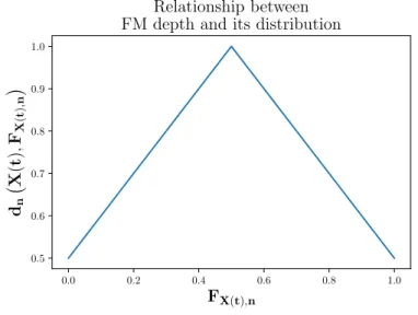
In Figure 2.3, the relationship between the cumulative distribution function and the depth defined in 2.6 can be seen. Note the maximum depth value is obtained at the median for any distribution considered. 0.0 0.2 0.4 0.6 0.8 1.0 FX(t),n 0.5 0.6 0.7 0.8 0.9 1.0 dn X ( t ) , FX ( t ) , n Relationship between FM depth and its distribution
Figure 2.3:Relationship between Fraiman and Muniz depth and the cumulative distribution function considered.
Applying Equations2.3and2.6, one possible implementation for multivariate stochastic processes using Fraiman and Muniz definition is the following:
dn(X, FX) = q X i=1 Z I d(Xi(t), FXi(t))∗w(t)dt ∗pi = q X i=1 Z I 1− 1 2−FXi(tj),n ∗w(t)dt ∗pi (2.7)
It is a weighted average of the depth values of each of the dimensions of the image, in turn, this depth values are calculated as integrals of pointwise data depth values.
2.1.2.
Band Depth and Modified Band Depth
Other implemented measure is the Band Depth (BD) introduced by López-Pintado and Romo (2009) [15] which is based on the graphic representation of functions. It makes use of the bands defined by their graphs on the plane. First, the original proposal for univariate processes is explained and the one for multivariate functional data later on.
Let remind the definition of graph of a function, a realization of a stochastic processX, G(X) = {(t, X(t)) :t∈I}. Then, the band inR2delimited byhcurvesXi1, Xi2, ..., Xih is defined as:
B(Xi1, Xi2, ..., Xih) = (t, X(t)) :t∈I, m´ın r=1,...,hXir(t)≤X(t)≤r=1m´ax,...,hXir(t) . (2.8)
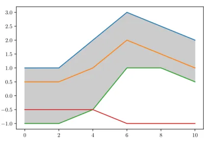
The grey area in Figure2.4is the band delimited by the blue and green curves, but it is also the band delimited by three curves: the blue, the orange and the green. For any functionXin the sample composed of curvesX1, X2, ..., Xn, the quantity
Sn(h)(X) = n h X 1≤i1≤...≤ih≤n I{G(X)⊂B(Xi1, Xi2, ..., Xih)}, 2≤h≤n, (2.9)
denotes the proportion of bands B(Xi1, Xi2, ..., Xih) determined by h different curves containing
the graph ofX, whereIis the indicator function. By computing the fraction of the bands containing the
curveX, the bigger the value of band depth, the more central position the curve has. With Equation2.9, the band depth function of a trajectory is defined as:
dn,H(X, FX,n) = H X h=2
2.1. FunctionalDepth
As a consequence, using Equation 2.4, the multivariate functional band depth function [16] forq -dimensional data is given by:
dn,H(X, FX,n) = q X j=1 pj H X h=2 S(nh)(Xj), 2≤H ≤n. (2.11)
López-Pintado and Romo (2009) [15] also proposed a more flexible definition of the band depth, the Modified Band Depth (MBD). Instead of using the indicator function in Equation2.9, the proportion of time the curve is inside the band is measured. It becomes:
Sn(h)(X) = n h X 1≤i1≤...≤ih≤n λk{A(X;Xi1, Xi2, ..., Xih)}, 2≤h≤n, (2.12) whereA(X;Xi1, Xi2, ..., Xih) ={t∈I : m´ınr=1,...,hXir(t)≤X(t)≤m´axr=1,...,hXir(t)}andλk= λ{A(X;Xi1, Xi2, ..., Xih)}/λ{I}, whereλ{·}is the Lebesgue measure.
The MBD is more convenient to obtain representative curves in terms of magnitude since less ties occur in terms of depth values among the observations. On the other hand, the band depth is preferred to detect shape differences. If curves do not intersect between them, the MBD turns out to give the same values as the band depth.
0 2 4 6 8 10 −1.0 −0.5 0.0 0.5 1.0 1.5 2.0 2.5 3.0 Example BD amd MBD
Figure 2.4:Basic example of BD and MBD applied to a dataset composed of four curves.
Differences between the BD and the MBD are illustrated with a simple example in Figure2.4. It is composed of 4 observations (n = 4) andH = 2, so there are 6 bands, one for every pair of curves. First, note that each curve belongs to those bands that delimits. Furthermore, it can be observed that the orange curve is completely inside other two bands (blue-green and blue-red), consequently, its BD
is 5/6. On the other hand, the other three curves are not inside any other band resulting in 0.5 their depth value. The MBD values for the blue and orange observations stay the same since they do not intersect with other curves. However, the red observation belongs to the grey band 40 % of the time, so its MBD value consists of(3 + 0,4 + 0,4)/6 = 0,63, where the three comes from the three bands it is border of, and the two 0.4 of the proportion of time it spends in the green-blue and green-orange bands. Likewise the MBD of the green observation is(3 + 0,6 + 0,6)/6 = 0,7.
2.2.
Functional Boxplot
Sun and Genton (2011) [17] introduced functional boxplots to visualize the result of ranking. Other informative exploratory tools include the rainbow plots and bagplots proposed by Hyndman and Shang (2010) [7] and the outliergram by Arribas-Gil and Romo (2013) [18]. The functional boxplot is an ex-tension of the classical boxplot which displays five statistics: the median, the first and third quartiles and the non-outlying maximum and minimum observations; and indicates the outlying observations. Its construction is based on depth measures which define the order statistics and consequently, the functional quantiles.
Analogously to the classical boxplot, the descriptive statistics shown in this plot include the 50 % central envelope, the median and the maximum non-outlying envelope. The 50 % central envelope, or 50 % central region, could be compared to the box of the classical boxplot which represents the interquartile range (IQR). More formally, theα-central region,Cα, 0 ≤ α ≤ 1, is delimited by the α proportion of deepest curves:
Cα= (t, y) :t∈Tk, m´ın r=1,...,dα·neX (r)(t)≤y≤ m´ax r=1,...,dα·neX (r)(t) , (2.13)
wheredα·nerepresents the smallest integer not less thanα·n. The median, as mentioned in the previous section, isX(1), the most central curve with the largest depth value. It is always found inside
the 50 % central region. It is a robust statistic to measure centrality.
The maximum non-outlying envelope is indicated by the whiskers (vertical lines extending from the box. The maximum non-outlying envelope is composed of the highest values (without taking into account outliers) found at each design point. So first, the outliers must be identified. The cutoff values are the fences obtained by inflating the the borders of the central regionC0,5 by 1.5 times the range of
theC0,5. The observations outside the fences are flagged as outliers.
In Figure2.5(a), a dataset composed of ten random realizations of a Brownian process is shown. Alongside, in2.5(b), the functional boxplot built from this data can be found. The median is plotted in black, the envelopes and the vertical lines in blue, theC0,5 in pink and the outliers in red. Note that only
2.2. FunctionalBoxplot
the median and the outliers are real observations.
0.0 0.2 0.4 0.6 0.8 1.0 2.0 1.5 1.0 0.5 0.0 0.5 1.0 1.5 2.0
Brownian process
(a) Raw data
0.0 0.2 0.4 0.6 0.8 1.0 2.0 1.5 1.0 0.5 0.0 0.5 1.0 1.5
2.0
Example Functional Boxplot
(b) Functional boxplot
Figure 2.5: On the left, a dataset composed of ten random realizations of a Brownian process is represented and on the right figure its boxplot.
The resulting functional boxplot reveals useful information when looking at their shape, length, po-sition and size. The spacings between the different parts of the box, intuitively indicate the degree of dispersion and skewness in the data. Note that in the functional context, robust methods are possibly more useful than in multivariate problems since there are more ways in which outliers affect functional statistics. A curve could be an outlier without having any unusually large value; besides magnitude, shape is also important.
0.0
0.2
0.4
0.6
0.8
1.0
2.0
1.5
1.0
0.5
0.0
0.5
1.0
1.5
2.0
Example Enhanced Boxplot
Figure 2.6:Enhanced boxplot of the dataset shown in2.5(a). The darkest pink color represents the
C0,75while the lightest, theC0,25
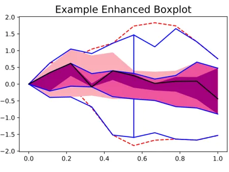
Moreover, there exists an enhanced functional boxplot in which the 25 % and 75 % central regions
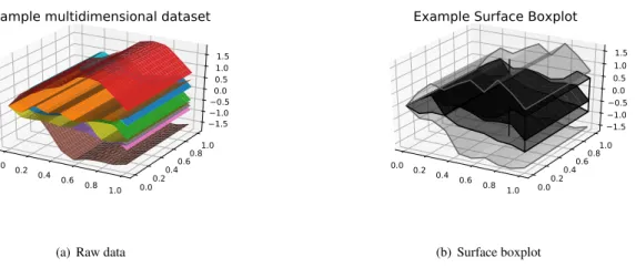
are provided as well (Figure2.6) and a surface boxplot [19], in whichI ⊂R2. To illustrate the surface
boxplot, a functional dataset with a two-dimensional domain space was generated extending the values of the dataset shown in2.5(a) along other axis, resulting in 2.7(a). Its surface boxplot is included in 2.7(b). 0.0 0.2 0.4 0.6 0.8 1.0 0.00.2 0.40.6 0.81.0 1.51.0 0.5 0.00.5 1.0 1.5
Example multidimensional dataset
(a) Raw data
0.0 0.2 0.4 0.6 0.8 1.0 0.00.2 0.40.6 0.81.0 1.51.0 0.5 0.00.5 1.01.5
Example Surface Boxplot
(b) Surface boxplot
Figure 2.7:A dataset of multidimensional functional data is shown alongside its surface boxplot.
2.3.
Magnitude-Shape Plot
Outliers in functional spaces are difficult to detect due to the diverse characteristics to consider. There are two big families of outliers: magnitude outliers (flagged by the boxplot) and shape outliers (the boxplot is inadequate). As a consequence, other tools are needed.
Dai and Genton (2018) [20] [21] contributed to the functional data toolbox with the magnitude-shape plot. It is another graphic method that helps visualizing both magnitude and magnitude-shape outlyingnes of univariate and multivariate functional data. Given a functional dataset, the shape outlyingness of these functional data is found on the vertical axis, while both the level and the direction of the magnitude outlyingness are plotted on the horizontal axis or plane. Moreover, it provides a criterion to identify various types of outliers that could lead to severe biases in modeling or forecasting functional data. Directional outlyingness
Note that outlyingness functions are equivalent to statistical depths in an inverse sense. If the depth function for a multivariate random variable X(t) with distribution function FX(t) is denoted by
d X(t), FX(t)
, its outlyingess is given by: o X(t), FX(t)
= 1
d X(t), FX(t)
2.3. Magnitude-ShapePlot
The magnitude-shape plot measures centrality of functional data by considering both level and di-rection of deviation from the central region. It adds didi-rection to the conventional concept of outlyingness, which is crucial in describing centrality of multivariate functional data [22]. To capture both magnitude and direction of outlyingness, direction is added to the outlyingness function as follows:
O X(t), FX(t) =o X(t), FX(t) ·v(t) = ( 1 d X(t), FX(t) −1 ) ·v(t), (2.15)
wheredcan be any conventional depth measure, andv(t) = (X(t)−Z(t))/kX(t)−Z(t)k, being
Z(t)the unique median ofFX(t)with respect todand|| · ||is theL2norm. In other words,vis the unit
vector pointing fromZ(t)toX(t)and basically, indicates the spatial sign of{X(t)−Z(t)}. For functional data, there are 3 different measures of directional outlyingness:
1. Mean directional outlyingness (MO):
MO(X, FX) = Z
I
O X(t), FX(t)·w(t)dt (2.16)
w(t) is a weight function defined on I. MO describes the relative position, both distance and direction, ofX on average to the center curve. Its norm,||MO||, is regarded as the magnitude outlyingness ofX.
2. Variation of directional outlyingness (V O): V O(X, FX) =
Z Ik
O X(t), FX(t)−MO(X, FX)k2·w(t)dt (2.17)
It measures the change of O X(t), FX(t)in terms of both the norm and direction across the whole interval. It is regarded as shape outlyingness. Functional data are usually classified by their shapes rather than scales because variation outlyingness accounts for both pointwise outlyin-gness and change in their directions.
3. Functional directional outlyingness (F O): F O(X, FX) = Z Ik O X(t), FX(t) k2·w(t)dt (2.18)
It represents the total outlyingness and the concept is similar to the the one of classical functional depth. However, classical functional depth mapsX∈C(I,Rq)to the compact interval[0,1]∈R
whereas the functional directional outlyingess mapsX to MOT, V O ∈ Rq×R+ which gives
more flexibility to analyze curves.
The functional directional outlyingness is linked to the other first two measures with the relationship: F O(X, FX) =kMO(X, FX)k2+V O(X, FX) (2.19)
The above decomposition of the functional directional oulyingness in magnitude and shape provides great flexibility for describing centrality of functional data and diagnosing potentially abnormal curves. When the curves are parallel, the shape otlyingness(V O)is zero and a quadratic relationship can be observed between the functional and magnitude outlyingness:F O=kMOk2.
The magnitude-shape plot indeed shows a scatter group of points MOT, V O for a sample of functional data. It is used to illustrate the centrality of curves with a response space up to two dimen-sions. When the dimension is higher, the points are defined by kMOkT, V O. The overall magnitude outlyingness is still presented, however the shape outlyingness is shown without direction.
1.0 1.2 1.4 1.6 1.8 2.0 0.6 0.4 0.2 0.0 0.2 0.4 0.6 0.8
Raw Data
(a) Esta es una subfigura1
6 4 2 0 2 4 6
MO
0.0 0.5 1.0 1.5 2.0 2.5 3.0VO
MS-Plot
(b) Esta es otra subfigura2
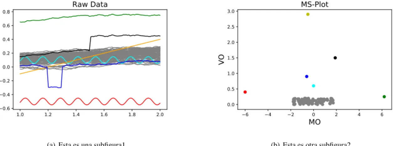
Figure 2.8:A group of curves with various types of outliers and its MS-plot.
In Figure 2.8 a functional dataset is plotted alongside its corresponding magnitude-shape plot to illustrate the basic concepts. The cluster of grey points found in the below mid-part of the graph corres-ponds to the central curves; both magnitude and shape outlyingness are small. In the vertical axis the variation outlyingness is plotted, so shape outliers appear on the top part of the graphic. The magnitude outlyingness is plotted on the horizontal axis, so shifted outliers appear on the sides of the graphic. The side is decided according the direction of their shifts.
Additionally, the magnitude shape plot provides a frontier to separate regular data from outliers. The outlier detection method is designed with the directional outlyingness, more specifically, using the empirical discrete form of the magnitude and the shape outlyingness,MOTk,nandV OTk,nrespectively.
MOTk,n(Xn, FX,n) = k X i=1 On X(ti), FX(ti),n ·wn(ti). (2.20)
2.4. ClusteringAlgorithms
The directional outlyingness maps one q-variate curve to a (q + 1)-dimensional vector Yk,n =
MOTk,n
T, V O Tk,n
T
which is well approximated with a multivariate normal distribution when X is generated by a stationary Gaussian process. Hardin and Rocke (2005) results [23] can be used under these suppositions to detect potential outliers fromYk,n. These results are indicated in the following steps:
1. Calculate the square robust Mahalanobis distance ofYk,nbased on a sample of sizeh≤n: RM D2Yk,n,Yek,n,J∗ =Yk,n,Ye∗k,n,J T S∗k,n,J−1Yk,n,Ye∗k,n,J , (2.21)
whereJ designates the group ohhpoints estimated by the Minimum Covariance Determinant al-gorithm, giving rise to the covariance matrixS∗
k,n,J = P i∈J Yk,n,i−Ye∗k,n,J Yk,n,i−Ye∗k,n,J T whereYek,n,J∗ =h−1Pi∈JYk,n,J.
2. Approximation of the tail of the distance distribution with a Fisher’sF distribution as follows: c(m−q) m(q+ 1)RM D 2Y k,n,Ye∗k,n,J ∼Fq+1,m−q ,
wherecandmare real numbers used to determine the degrees of freedom of theF distribution and the scaling factor.
3. Flag a curve as an outlier when its distance satisfies: c(m−q) m(q+ 1)RM D 2Y k,n,Yek,n,J∗ > C,
whereCis a cutoff value chosen as theα-quantile ofFq+1,m−q;α= 0,993is used in the classical boxplot for detecting outliers under a normal distribution.
2.4.
Clustering Algorithms
Functional depth also indicates how similar observations are and therefore, it can be used in fun-ctional classification and inference. For example, Flores, Lillo and Romo [24] used depth measures to perform homogeneity tests. Baillo, Cuevas and Fraiman [25] provide a survey of the literature concer-ning classification of functional data. This section is focused on some basic notions of clustering [26]. Cluster analysis is a collection of unsupervised classification techniques for grouping objects or seg-menting datasets into subsets of data called clusters. Clustering methods try to assign similar objects that share common characteristics into the same cluster.
There are three categories of clustering algorithms: hierarchical, non-hierarchical or flat, and a mixed approach. In practice, their use is limited to their complexity, efficiency or availability in current software. Furthermore, the choice of the algorithm to run on a certain dataset depends on the sample size, structure or even the proper goals of the cluster analysis.
The methods of the k-means family are non-hierarchical partitioninng algorithms with good cluste-ring results in shorter times and on larger datasets compared to hierarchical ones. As a consequence, they are the most popular algorithms found in exploratory analysis and data mining applications.
By using a clustering algorithm, the datasetX={X1,X2, , ...,Xn}is divided intokgroups aiming at obtaining low within-cluster and high between-cluster heterogeneity. In other words, a cluster contains objects as similar to each other as possible and as far from other objects in other clusters as possible. To measure the closeness of the observations, a distance measure is needed. Usually, the standard L2 distance is used but the distance can be calculated using statistics based on depth measures. The
parameter indicating the number of clusters,k, is known or fixed a priori before running the algorithm. Clusters are described by their member objects and by their centers, which are usually the centroids. A centroid is the point that minimizes the sum of distances between itself and each point in the cluster. The prototype vector of cluster centroids is denoted byC= [C1,C2, ...,Cn],Ci∈Rd.
2.4.1.
K-means
K-means (KM) , or alternatively Hard C-Means, is an iterative clustering algorithm that computes clusters in order to minimize the sum of distances from each object to its cluster centroid. In other words, the following function must be minimized:
JKM(X;C) = c X i=1 ni X j=1 D2ij, c X i=1 ni=n, (2.22)
where ni indicates the number of observations in the ith cluster and Dij denotes the distance chosen between thejthobservation and theithcenter.
In each iteration, the observations are reassigned between clusters until a minimum point ofJKM is reached. The algorithm steps are captured in 2.1. The random function indicates the selection of krandom trajectories fromX, distancecalculates the distance between observation units and cluster centroids, the partition method assigns each observation to the cluster of the closest centroid and
centroidsupdates the centroids using:Ci= n1iPjn=1i Xj, for1≤i≤k.
K-means is a fast, robust, and easy to implement algorithm. It assigns each object to exactly one cluster, so it gives comparatively good results if clusters are distinct or well-separated. Nevertheless, it is not as reliable in finding overlapping clusters with regard to form or scattering. Also, it fails to cluster
2.4. ClusteringAlgorithms
input : X, optionally C
output: P(array of lengthn): a partition of X, C 1 C← Cor random( X); 2 cond← true; 3 while cond do 4 Cold← C; 5 D← distance( C, X); 6 P← partition( D, X); 7 C← centroids( P, X); 8 cond← not_equal( C, Cold); 9 end
Algorithm 2.1:K-means algorithm.
noisy data and is not invariant to non-linear transformations of data.
2.4.2.
Fuzzy K-means
The Fuzzy K-means (FKM), or Soft C-Means, algorithm is an extension of KM that was introduced to overcome the aforementioned disadvantages of KM. It is a soft algorithm clustering fuzzy data and it assigns each object to different clusters with varying degrees of membership. These values range bet-ween 0 and 1. It is used in a wide area of applications although it has a relatively higher computational cost.
Analogously toKM, the Fuzzy K-Means computes clusters iteratively in order to minimize the follo-wing function: JF KM(X;U,V) = k X i=1 n X j=1 umij ·Dij2. (2.23)
The difference with respect to KM is the used of weighted square errors. U is the membership matrixk×nthat represents the fuzzy clustering of the datasetX. Each of its entrances,uij, indicates the membership value of thejthobservation to theithcluster.mis the fuzzifier parameter or weighting exponent,m∈[1,∞). Asmapproaches to 1, the clustering tends to become crisp, on the contrary, as m goes to∞, the clusering becomes fuzzified. It is usually fixed as 2.
Fuzzy K-Means must be run under these three constrainsts: 1. uij ∈[0,1], 1≤i≤k and 1≤j ≤n,
2. Pki=1uij = 1, 1≤j≤n, 3. 0<Pnj=1uij < n, 1≤i≤k.
The algorithm can be found in2.2, in which therandomanddistance functions are the same as in
KM. Themembership_values method calculates the membership values of data points to each cluster with:uij =hPkc=1(Dij/Dcj)
2 m−1
i−1
, 1 ≤i≤kand1 ≤j ≤ nand thecentroids function updates the centroids using:Ci =
Pn j=1u m ijXj Pn j=1umij , 1≤i≤k . input : X, optionally C output: U, C 1 C← Cor random( X); 2 cond← true; 3 while cond do 4 Cold← C; 5 D← distance( C, X); 6 U← membership_values( D, X); 7 C← centroids( U, X);
8 cond← not_equal( C, Cold); 9 end
Algorithm 2.2:Fuzzy K-means algorithm.
There are many other approaches to cluster data, for example using the coefficients of the B-Splines basis [27] instead of the actual observation values or the SeqClusFD algorithm in which the functional boxplot is involved [28].
3
S
oftware
D
evelopment
P
rocess
In the previous section, the core functionalities implemented were exposed in detail. In this one, the development of the Python package,scikit-fda, is going to be explained. First of all, an agile met-hodology which uses incremental, iterative work cycles was followed. These cycles were assessed by the developing team in regular meetings which were hold every week. In each cycle the phases of the Waterfall model (requirements analysis, software design, implementation, testing and integration) were completed for a specific functionality, before proceeding to the next increment.
3.1.
Analysis
The package requirements were already specified from the beginning of the project started last year by former student Miguel Carbajo [9]. However, an overview is given to remind the main ones. The pac-kage is written in Python. It is a general purpose language and multi-paradigm, which implies flexibility in the implementations of a technique. Moreover, it is great for prototyping due to the dynamic typing and the possibility to use it as a Read-Eval-Print-Loop (REPL) with for example, Jupyter Notebooks. In addition, it has a rich ecosystem with a great variety of modules in different fields. Pandas can be found for statistical calculations, Matplotlib for plotting and, Numpy and Scipy stand out in Python scientific computing modules. Algorithms which are already implemented in those last packages can be reutili-zed and assure efficiency due to the lower-level languages they are programmed in, such as Fortran or C. Numpy adds support for large, multi-dimensional arrays and matrices, along with a large collection of high-level mathematical functions to operate on these arrays. SciPy contains modules for optimization, linear algebra, integration, interpolation and other tasks common in science and engineering. Moreover, SciPy builds on the NumPy array object.
The package must be integrated with Python science environment, therefore, it follows scikit-learn API. Scikit stands for Scipy-Toolkits which are specialized science add-on packages for Scipy. They are developed separately and independently from the main distribution.
Furthermore, it is an open-source, scalable, software package which implies the presence of an easy mechanism to contribute to it, along with an extensive test-bench of unit tests and continuous
integration procedures. Also, documentation is important both for the general audience the package is intended for and the potential developers of the package.
8
exploratory
analysis
representation
preprocessing
statistical inference
machine learning
scikit-fda
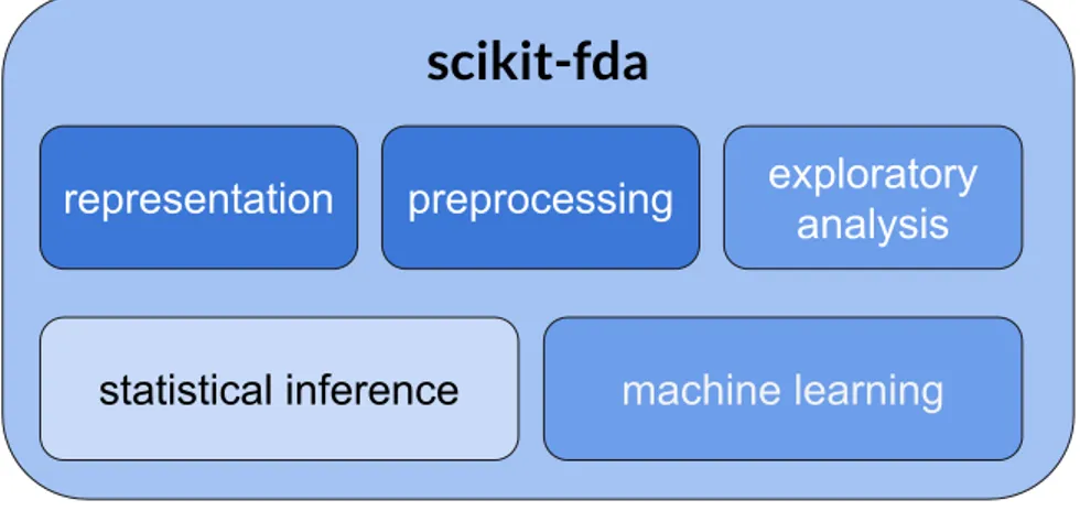
Figure 3.1:Division of scikit-fda functionality. The intensity of the colors reflects the level of functio-nality implemented, being the area of inference the one which requires more contribution.
Finally, the goal is to include as much functionality as possible to cover the areas shown in Figure3.1 [29]. Regarding this project, the functionality implemented is proportional to the 360 hours of a degree work and it was decided just after each cycle. The specific analysis for the functionalities implemented consisted basically in researching to decide what to include in the package, both in the mathematical and computer science fields, to determine the most innovative, popular and viable methods.
3.2.
Design
As commented in the Introduction1.1, the package in its initial version included two modules con-taining both representations of functional data, as a grid (FDataGrid) or as a linear combination of basis functions (FDataBasis); along with a basicmathmodule and a couple related tosmoothingtechniques. During this year, the package structure has considerably grown due to the number of people working on it. The following paragraphs describe the implementation of the concepts explained in Chapter2. Depth Measures
The three implemented depth functions: Fraiman and Muniz depth, Band depth and Modified Band depth, can be found in thedepthmodule. This module is found in theexploratory analysisdirectory due to its applications. The three methods follow the signature depth_name(fdatagrid, pointwise=False), where the first argument expects a FDataGrid object and the second one indicates wether to return also the pointwise univariate depth. The second parameter was added because, by default, in Equation 2.3, w(t) = 1/|Tk|, 1 ≤ j ≤ k and pi = 1/q, 1 ≤ i ≤ q. So, if the functional result is desired to be calculated with other weight values, it is possible to obtain it from the pointwise univariate depth.
3.2. Design
Besides, the code is scalable since the adding of a new method does not imply to modify anything. Regarding the BD and MBD, in Equation2.10the number of curves determining a band,h, can be any integer between 2 andH. The order of curves induced by the depths are very stable in H. So to avoid computational issues,H = 2is used because a fast method was proposed by Sun and Genton (2012) [30] based on matrix (or, in higher dimensions, tensor) ranks. The pseudocodes of both functions are included. Both of them assume univariate functional datasets represented in a matrixM, n×k. In 3.1,na[i]denotes the number of curves that are completely above theithcurve, whereasnb[i]denotes the number of curves that are completely below the ith curve, 1 ≤ i ≤ n. na, nb and depth aren -dimensional vectors. In3.2,na,nb andmatcharen×kmatrices whiledepthstays the same, a vector of lengthn. input :M output:depth 1 foreach j←1 tok do 2 R[,j]←rank(M[,j]); 3 end 4 foreach i←1 ton do 5 na[i]←n - max(R[i,]); 6 nb[i]←min(R[i,])- 1; 7 end
8 depth←(na * nb + n- 1) / nchoose2 ;
Algorithm 3.1:Band Depth pseudocode.
input :M output:depth 1 foreach j←1 tok do 2 R[,j]←rank(M[,j]); 3 end 4 na←n - R; 5 nb←R - 1; 6 match←na * nb; 7 foreach i←1 ton do 8 proportion←sum(match[i, ]) / k ; 9 end
10 depth←(proportion + n - 1) / nchoose2 ;
Algorithm 3.2:Modified Band Depth pseudocode.
Boxplot
The boxplot functionality is implemented in two classes: Boxplot and SurfaceBoxplot. They can be found in the boxplot module, inside the visualization directory which in turn can be found in the
exploratory analysis one. Both classes support FDataGrid objects with as many dimensions on the
image as desired whereas the first class only admits one dimensional domains and the second one bidimensional domains. A graph for each dimension on the image is returned, so domain spaces only have sense up to two dimensions.
Both classes inherit from an abstract one, FDataBoxplot, whose attributes contain the descriptive statistics: median, central_evelope and outlying_envelope. To calculate them, the depth function and the factor to identify outliers can be customized. By default, themodified_band_depth function and the value 1.5 for the factor are applied. To obtain the graphic, the plot function must be called, and the colormap used can be chosen. In interactive mode, the plot is the default representation of the class.
Although the procedure to obtain the mathematical results is very similar in both cases, the plotting part is quite different. In the first case, a line is plotted for each observation while in the second one, a surface is shown. For clarity reasons, the SurfaceBoxplot does not show outliers nor has the possibility to produce an enhanced boxplot as in the case of theBoxplot class. Indeed, in theBoxplot class, any αcentral regions can be selected to appear.
Magnitude-Shape Plot
This plot is implemented in a class named the same way, MagnitudeShapePlot, in the magnitu-de_shape_plot module found in the visualization directory. This module also contains the method to calculate the directional outlyingness of the FDataGrid object considered. This method is used by the MagnitudeShapePlot class in which the depth function, along with the dimension and pointwise weights, can be customized.
Once the directional outlyingnes has been computed, the mean and the variation of the directional outlyingness are calculated to obtain the actual points of the graphic. The norm implemented by default for Equations2.16,2.17and2.18is theL2-norm defined askfk =
R
I|f|2dx 1
2, wherek · k
∗ denotes
a vectorial norm (also theL2-norm by default).
Finally, the outliers are calculated using the MinCovDet class provided by scikit-learn and the cutoff value can be adjusted by means of the parameter alpha.
Clustering Algorithms
The clustering functionality can be found in theclusteringdirectory, insidemachine learning. Speci-fically, a module calledbase_kmeanswas created to include K-means algorithms: K-means and Fuzzy K-means, which are implemented in two classes named after them. Both classes inherit from BaseK-Means class which follows scikit-learn API with scrutiny. This latter class inherits from BaseEstimator, ClusterMixin and TransformerMixin contained in the aforementioned package and implements the fit,
transformandscoremethods among others. This implementation follows the one found in scikit-learn of the KMeans class, which uses vectorial L2-norm to compute distances. By default, the functional
3.3. Coding, Documentation andTesting
previous subsection), nevertheless, it admits any suitable distance function.
In order to visualize the results, a module namedclustering_plotslocated in thevisualization direc-tory was created. It includes three methods:plot_clusters,plot_cluster_linesandplot_cluster_bars. The first one plots the raw data by colors, in which each color indicates a cluster. The other two methods are applicable only for the Fuzzy K-means class results which help to visualize the degree of membership of each observation to each cluster, by means of a kind of parallel coordinates plot or histogram plot respectively.
3.3.
Coding, Documentation and Testing
Any open-source package needs to be composed of scalable source code in order for programmers to contribute in its development. It is always easier if there are guidelines that assure consistency and make the code more readable. As a consequence, standard PEP 8: The Style Guide for Python Code is followed. It contains coding conventions comprising the standard library in the main distribution, which include information about indentation, maximum line length (79 characters), blank lines, encodings (PEP 263) or naming conventions.
In turn, PEP 8 references PEP 257 standard for documentation. It describes docstrings (documen-tation strings) semantics and conventions. Docstrings are found at the beginning of all public modules, functions, classes and methods, and they should be kept short, simple and avoiding repetitions.
Another point to take into account for a collaborative software is testing in order to produce a quality product and detect bugs. The testing framework used is based onunittest, which is indeed the de facto standard in this area. It constitutes the Python language version of JUnit, Java’s testing framework. It supports test automation, sharing setup and shutdown code for tests, or aggregation of tests into co-llections. Nevertheless, the tool employed for running the tests ispytest, which contains more features, including more informative tracebacks, stdout and stderror capturing, or stopping after a fixed number of failures; and supports more complex functional testing.
Another positive aspect of following standards, is the existence of tools that automatize their use. Personally, I usedPyCharmto write the source code. It has a number of settings to configure the Python environment. The docstring format can be chosen among plain, reStructuredText, Epytext, Numpy or Google. The one selected is the Google standard which follows PEP8 and has a morepythonicsyntax. PyCharm can understand the docstrings, aid with their generation and use them for quick fixes and coding assistance.PyCharm also allows to configureSphinxworking directory.
Sphinxis a documentation generator that converts reStructuredText, an extensible, markup langua-ge used by the Python community for technical documentation, into HTML websites or other formats such as pdf. It autogenerates documentation from the source code, writing mathematical notation or
highlighting code. Moreover, it is linked withdoctest that tests the code by running the examples em-bedded in the documentation and verifies if the expected results were produced.
3.4.
Version Control and Continuous Integration
Due to the high number of potential contributors, there must be some kind of coordination among them. Fortunately, tools for version control are already spread. In this case,Git has been used. It is a distributed version-control system that tracks changes in the source code of any file during the software development and gives support to distributed, non-linear worflows. A Git directory is a repository with full history and version tracking abilities, independent of network or a central server access.
More specifically, the package can be found on GitHub, in https://github.com/GAA-UAM/ scikit-fda/wiki, a web-based hosting service using Git for version control. Apart from Git fun-ctionalities, it offers its own features which include access control and regarding collaboration between programmers, bug tracking, feature request or task management. The repository can be read and clo-ned but writing is controlled by the owners.
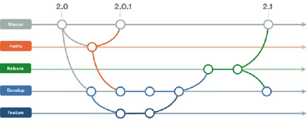
The Git flow is based on branches and supports teams and projects where deployments are made regularly. It consists on the following steps: create a branch from the repository, add commits, open pull request, discuss and review code, deploy for testing and finally, merge. The repository contains two main branches: amasterbranch in which the releases available can be found and thedevelopbranch, into which thefeaturebranches are merged during the development process.
Figure 3.2:Git flow.
GitHub also provides some software as a service integrations to add extra features to projects. Travis CI can be found among the hosted continuous integration services used to build and test software projects. It gives full control over the build environment to adapt it to the code and runs the tests every time a push is done. Testing is not a just one-time task. Additionally, it gives support to more than one version of Python simultaneously.
3.4. VersionControl andContinuousIntegration
Another hosting platform linked to GitHub isRead the Docswhich generates documentation com-piled with Sphinx. It simplifies the technical documentation by automatically building, versioning and hosting the generated documentation in its website. The package documentation can be foundhere.
4
R
esults
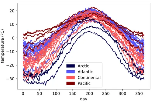
In this section the results of the functionality implemented are shown applied to the Canadian Weat-her dataset described in the introduction of Chapter 2. More specifically, only the temperatures are going to be studied, dealing with one dimensional functional data. The Canadian Weather dataset can be obtained from thedatasetsmodule. It contains functions to generate synthetic datasets or to retrieve specific datasets which are fetched from CRAN or UCR. In Figure4.1, the raw data is plotted to show the curves to be analyzed. They are divided according to the target. In this case, it includes the different climates to which the weather stations belong to: Arctic, Atlantic, Continental and Pacific.
0
50
100
150
200
250
300
350
day
30
20
10
0
10
20
temperature (ºC)
Arctic
Atlantic
Continental
Pacific
Canadian Temperatures
Figure 4.1:The temperatures of the Canadian Weather dataset.
Boxplot
The functional boxplot, Figure 4.2(a), is constructed based on this data. It can be observed the median in black, the central region (where the 50 % of the most central samples reside) in pink and the envelopes and whiskers in blue. The outliers detected, those samples with at least a point outside the
outlying envelope, are represented with a red dashed line. In the right plot, Figure4.2(b), the outliers (in red) are shown with respect to the other samples (in blue). Note their significantly lower values compared to the rest. This is the expected result due to the depth measure used, the modified band depth, which rank the samples according to their magnitude.
0 50 100 150 200 250 300 350 day 30 20 10 0 10 20 temperature (ºC) Canadian Temperatures
(a) Functional boxplot
0 50 100 150 200 250 300 350 day 30 20 10 0 10 20 temperature (ºC) nonoutliers outliers Canadian Temperatures
(b) Outlier detection result
Figure 4.2:The boxplot applied to the Canadian temperatures and the distinction made of outler and regular curves.
If the band depth measure is used and other central regions are included, the result is shown in 4.3. The outliers detected belong to the Pacific and Arctic climates which are less common to find in Canada. As a consequence, this measure detects better shape outliers compared to the previous one.
0
50
100
150
200
250
300
350
day
30
20
10
0
10
20
temperature (ºC)
Canadian Temperatures
Magnitude-Shape Plot
Following the previous example, Figure 4.4 shows the magnitude-shape plot applied to the data along with its detected outliers plot. The band depth measure was used. Most of the curves pointed as outliers belong either to the Pacific or Arctic climates, not so common in Canada. The Pacific temperatu-res are much smoother and the Arctic ones much lower, differing from the temperatu-rest in shape and magnitude respectively. There are two curves from the Arctic climate which are not pointed as outliers but in the MS-Plot, they appear further left from the central points.
15 10 5 0 5 MO 0 10 20 30 40 VO MS-Plot (a) MS-Plot 0 50 100 150 200 250 300 350 day 30 20 10 0 10 20 temperature (ºC) nonoutliers outliers Canadian Weather
(b) Outlier detection result
Figure 4.4:Magnitude-Shape plot applied to the Canadian temperature data along with its detected outliers plot. The Modified Band depth is used.
In Figure4.5, the same experiment is carried out but with the Fraiman and Muniz depth measure. The actual MS-Plot does not point out any observation as an outlier. Nevertheless, if we group them in three groups according to their position in the MS-Plot, the result is the expected one. Those samples at the left (larger deviation in the mean directional outlyingness) correspond to the Arctic climate, which has lower temperatures, and those on top (larger deviation in the directional outlyingness) to the Pacific one, which has smoother curves. The same is done with the MBD in Figure4.6.
0.8 0.6 0.4 0.2 0.0 0.2 0.4 0.6 0.8 magnitude outlyingness 0.00 0.05 0.10 0.15 0.20 0.25 0.30 shape outlyingness MS-Plot
(a) Groupings of the MS-Plot points.
0 50 100 150 200 250 300 350 day 30 20 10 0 10 20 temperature (ºC) Canadian Weather
(b) Raw data according to the groupings.
Figure 4.5: Magnitude-Shape plot applied to the Canadian temperature. The Fraiman and Muniz depth is used. The points are divided into three groups.
15 10 5 0 5 magnitude outlyingness 0 10 20 30 40 shape outlyingness MS-Plot
(a) Groupings of the MS-Plot points.
0 50 100 150 200 250 300 350 day 30 20 10 0 10 20 temperature (ºC) Canadian Weather
(b) Raw data according to the groupings.
Figure 4.6:Magnitude-Shape plot applied to the Canadian temperature. The MBD is used. The points are divided into three groups.
Clustering Algorithms
For the cluster analysis, the sample to be investigated consists in ten observations picked randomly from the above dataset. Figure4.7(a)shows the raw data.
0 50 100 150 200 250 300 350 day 30 20 10 0 10 20 temperature (ºC) Atlantic Continental Pacific Canadian Weather
(a) Ten random observations of the Canadian Weather dataset.
0 50 100 150 200 250 300 350 day 30 20 10 0 10 20 temperature (ºC) Atlantic Pacific Continental Canadian Weather
(b) Raw data according to clusters. Cluster centroids are represented with the same colors and bigger linewidth.
Figure 4.7:Ten random observations of the Canadian Weather dataset and its division into three different clusters.
Note the ten curves chosen belong to three of the four possible climates. The number of clusters is set to three since there are three pronounced distinctions regarding form. Although the three groups are composed of bell-shaped curves, the continental ones are more acute and one of the Pacific climate is considerably shallower. The K-means results are plotted in Figure4.7(b). The Fuzzy K-Means algorithm produces the same results as in Figure4.7(b)if assigning to each observation the cluster with maximum degree of membership. The groupings have been made according to shape and magnitude.
Furthermore, two other ad-hoc plots have been implemented to better visualize every degree of membership of each observation. One of them appears in Figure4.8and is similar to parallel
coordina-Atlantic
Pacific
Continental
Cluster
0.0
0.2
0.4
0.6
0.8
1.0
Degree of membership
Degrees of membership of the samples to each cluster
Figure 4.8:Plot implemented to show Fuzzy C-means algorithm results.
tes. The colors are the ones of the first plot (Figure4.7(a)), dividing the samples by actual climate. The other one, Figure 4.9, returns a barplot. Each sample is designated with a bar which is filled proportionally to its membership values with the color of each cluster.
0 1 2 3 4 5 6 7 8 9 0.0 0.2 0.4 0.6 0.8 1.0 Atlantic Pacific Continental
Degrees of membership of the samples to each cluster
(a) Without ordering.
7 1 4 8 0 5 3 2 9 6 0.0 0.2 0.4 0.6 0.8 1.0 Atlantic Pacific Continental
Degrees of membership of the samples to each cluster
(b) Ordered based to the Pacific climate.
Figure 4.9:Plot implemented to show Fuzzy K-means algorithm results.
5
F
uture
W
ork and
C
onclusions
Figure 5.1:scikit-fda logo
Along the document, depth measures and its applications have been explained. Both a theoretic introduction and an implementation have been included. In addition, the final graphic results have been exposed. In regard with this more specialized area, more depth measures could be incorporated. There are many heterogeneous notions of depths which can give rise to different outputs in terms of the cha-racteristic considered. The package could also contain other exploratory tools such as the mentioned outliergram, bagplot or rainbow plot, as well as, an extension of the MS-Plot to a higher dimension. Furthermore, distance measures could be built using the depths defined and more cluster techniques could be added.
In parallel, other two students were working in the project. They focused in preprocessing, which in-cludes smoothing and registration techniques. These techniques approximate functions in order to deal with registered noise and variation in phase and amplitude, respectively. Also, some basic regression methods have been included to model the data. Regarding Figure3.1with the expected functionality of the package, more effort must be invested especially in statistical inference such as estimation and hypothesis testing of functional data.
Still the outcome of the project has accomplished the expectations. The final goal of the thesis was to develop a comprehensive Python package for Functional Data Analysis. So firstly, the functionality of the fda package initiated last year had to be expanded. A lot of work has been invested, not only by me but also by the other team members. This implied great collaboration which could be achieved thanks to communication in regular meetings and via GitHub, a very useful tool which helped in the coordination
and regulation of the team regarding to code implementation. It also allows the supervision and approval of merge requests and the addressing of issues. Moreover, its integration with Travis CI allows to follow the continuous integration practice. Testing and documentation are also monitorized through GitHub web service.
Not so much along, the first release of the package was delivered under the name ofscikit-fda. It has a BSD license and the logo is the one in Figure 5.1. The long term goal is to implement novel techniques so that the Python fda package evolves together with the field of Functional Data Analysis.
B
ibliography
[1] J. O. Ramsay and B. W. Silverman, Functional data analysis. Springer series in statistics, New York: Springer, 2nd. ed., 2005.
[2] F. Ferraty and P. Vieu,Nonparametric functional data analysis: theory and practice. Springer series in statistics, New York: Springer, 2006.
[3] J. O. Ramsay and B. W. Silverman, “Functional data analysis - Software.”http://www.psych.
mcgill.ca/misc/fda/software.html, 2017.