Episodic Training for Domain Generalization

000 001 002 003 004 005 006 007 008 009 010 011 012 013 014 015 016 017 018 019 020 021 022 023 024 025 026 027 028 029 030 031 032 033 034 035 036 037 038 039 040 041 042 043 044 045 046 047 048 049 050 051 052 053 054 055 056 057 058 059 060 061 062 063 064 065 066 067 068 069 070 071 072 073 074 075 076 077 078 079 080 081 082 083 084 085 086 087 088 089 090 091 092 093 094 095 096 097 098 099 100 101 102 103 104 105 106 107

Episodic Training for Domain Generalization

Anonymous ICCV submission

Paper ID 1488

Abstract

Domain generalization (DG) is the challenging and topi-cal problem of learning models that generalize to novel testing domains with different statistics than a set of known training do-mains. The simple approach of aggregating data from all source domains and training a single deep neural network end-to-end on all the data provides a surprisingly strong baseline that sur-passes many prior published methods. In this paper we build on this strong baseline by designing an episodic training procedure that trains a single deep network in a way that exposes it to the domain shift that characterises a novel domain at runtime. Specifically, we decompose a deep network into feature extrac-tor and classifier components, and then train each component by simulating it interacting with a partner who is badly tuned for the current domain. This makes both components more robust, ultimately leading to our networks producing state-of-the-art performance on three DG benchmarks. Furthermore, we con-sider the pervasive workflow of using an ImageNet trained CNN as a fixed feature extractor for downstream recognition tasks. Using the Visual Decathlon benchmark, we demonstrate that our episodic-DG training improves the performance of such a general purpose feature extractor by explicitly training a feature for robustness to novel problems. This shows that DG training can benefit standard practice in computer vision.

1. Introduction

Machine learning methods often degrade rapidly in perfor-mance if they are applied to domains with very different statistics to the data used to train them. This is the problem of domain shift, which domain adaptation (DA) aims to address in the case where some labelled or unlabelled data from the target domain is available for adaptation [2,35,21,10,22,4]; and domain gen-eralisation (DG) aims to address in the case where no adaptation to the target problem is possible [26,12,18,32] due to lack of data or computation. DG is a particularly challenging problem setting, since explicit training on the target is disallowed; yet it is particularly valuable due to its lack of assumptions. For example, it would be valuable to have a domain-general visual feature extractor that performs well ‘out of the box’ as a

representation for any novel problem, even without fine-tuning. The significance of the DG challenge has led to many stud-ies in the literature. These span robust feature space learning

[26,12], model architectures that are purpose designed to

en-able robustness to domain shift [16,38,17] and specially de-signed learning algorithms for optimising standard architectures

[32,18] that aim to fit them to a more robust minima. Among

all these efforts, it turns out that the naive approach [17] of aggregating all the training domains’ data together and train-ing a strain-ingle deep network end-to-end is very competitive with state-of-the-art, and better than many published methods – while simultaneously being much simpler and faster than more elabo-rate alternatives. In this paper we aim to build on the strength and simplicity of this simple data aggregation strategy, but improve it by designing an episodic training scheme to improve DG.

The paradigm of episodic training has recently been popularised in the area of few-shot learning [9,27,33]. In this problem, the goal is to use a large amount of background source data, to train a model that is capable of few-shot learning when adapting to a novel target problem. However despite the data availability, training on all the source data would not be reflective of the target few-shot learning condition. So in order to train the model in a way that reflects how it will be tested, multiple few-shot learning trainingepisodesare setup among all the source datasets [9,27,33].

How can an episodic training approach be designed for domain generalisation? Our insight is that, from the perspective of any layerlin a neural network, being exposed to a novel domain at testing-time is experienced as that layer’s neighbours

l−1orl+1being badly tuned for the problem at hand. That is, neighbours provide input to the current layer (or accept output from it) with different statistics to the current layer’s expectation. Therefore to design episodes for DG, we should expose layers to neighbours that are untrained for the current domain. If a layer can be trained to perform well in this situation of badly tuned neighbours, then its robustness to domain-shift has increased.

To realise our episodic training idea, we break networks up into feature extractor and classifier modules and train them with our episodic framework. This leads to more robust modules that together obtain state-of-the-art results on several DG benchmarks. Our approach benefits from end-to-end

108 109 110 111 112 113 114 115 116 117 118 119 120 121 122 123 124 125 126 127 128 129 130 131 132 133 134 135 136 137 138 139 140 141 142 143 144 145 146 147 148 149 150 151 152 153 154 155 156 157 158 159 160 161 162 163 164 165 166 167 168 169 170 171 172 173 174 175 176 177 178 179 180 181 182 183 184 185 186 187 188 189 190 191 192 193 194 195 196 197 198 199 200 201 202 203 204 205 206 207 208 209 210 211 212 213 214 215

learning, while being model agnostic (architecture independent), and simple and fast to train; in contrast to most existing DG techniques that rely on non-standard architectures [17], auxiliary models [32], or non-standard optimizers [18].

Finally, we provide a practical demonstration of the value of explicit DG training, beyond the isolated benchmarks that are common in the literature. Specifically, we consider whether DG can benefit the common practitioner workflow of using an ImageNet [30] pre-trained CNN as a feature extractor for novel tasks and datasets. The standard (homogeneous) DG problem setting assumes shared label-spaces between source and target domain, thus highly restricting its applicability. To benefit the wider computer vision workflow, we go beyond this toheterogeneousDG (Table5). That is, to train a feature extractor specifically to improve its robustness in representing novel downstream tasks without fine-tuning. Using the Visual Decathlon benchmark [28], we show that Episodic training provides an improved representation for novel downstream tasks compared to the standard ImageNet pre-trained CNN.

2. Related Work

Multi-Domain Learning (MDL) MDL aims to learn sev-eral domains simultaneously using a single model [3,28,29,39]. Depending on the problem, how much data is available per domain, and how similar the domains are, multi-domain learning can improve [39] – or sometimes worsen [3,28,29] – performance compared to a single model per domain. MDL is related to DG because the typical setting for DG is to assume a similar setup in that multiple source domains are provided. But that now the goal is to learn how to extract a domain-agnostic or domain-robust model from all those source domains. The most rigorous benchmark for MDL is the Visual Decathlon (VD) [28]. We repurpose this benchmark for DG by training a CNN on a subset of the VD domains, and then evaluating its performance as a feature extractor on an unseen disjoint subset of them. We are the first to demonstrate DG at this scale, and in the heterogeneous label setting required for VD.

Domain Generalization Despite different details, previous DG methods can be divided into a few categories by motivat-ing intuition. Domain Invariant Features: These aim to learn a domain-invariant feature representation, typically by minimising the discrepancy between all source domains – and assuming that the resulting source-domain invariant feature will work well for the target as well. To this end [26] employed maximum mean discrepancy (MMD), while [12] proposed a multi-domain re-construction auto-encoder to learn this domain-invariant feature. More recently, [20] applied MMD constraints within the rep-resentation learning of an autoencoder via adversarial training. Hierarchical Models: These learn a hierarchical set of model parameters, so that the model for each domain is parameterised by a combination of a domain-agnostic and a domain-specific parameter [16,17]. After learning such a hierarchical model

structure on the source domains the domain agnostic parameter can be extracted as the model with the least domain-specific bias, that is most likely to work on a target problem. This intuition has been exploited in both shallow [16] and deep [17] settings. Data Augmentation: A few studies proposed data augmentation strate-gies to synthesise additional training data to improve the robust-ness of a model to novel domains. These include the Bayesian network [32], which perturbs input data based on the domain classification signal from an auxiliary domain classifier. Mean-while, [36] proposed an adversarial data augmentation method to synthesize ‘hard’ data for the training model to enhance its generalization. Optimisation Algorithms: A final category of approach is to modify a conventional learning algorithm in an at-tempt to find a more robust minima during training, for example through meta-learning [18]. Our approach is different to all of these in that it trains a standard deep model, without special data augmentation and with a conventional optimiser. The key idea requires only a simple modification of the training procedure to introduce appropriately constructed episodes. Finally, in contrast to the small datasets considered previously, we demonstrate the impact of DG model training in the large scale VD benchmark.

Neural Network Meta-Learning Learning-to-learn and meta-learning methods have resurged recently, in particular in few-shot recognition [9,33,24], and learning-to-optimize [27] tasks. Despite signifiant other differences in motivation and methodological formalisations, a common feature of these methods is an episodic training strategy. In few-shot learning, the intuition is that while lot of source tasks and data may be available, these should be used for training in a way that closely simulates the testing condition. Therefore at each learning iteration, a random subset of source tasks and instances are sampled to generate a training episode defined by a random few-shot learning task of similar data volume and cardinality as the model is expected to be tested on at runtime. Thus the model eventually ‘sees’ all the training data in aggregate, but in any given iteration, it is evaluated in a condition similar to a real ‘testing’ condition. In this paper we aim to develop an episodic training strategy to improve domain-robustness, rather than learning-to-learn. While the high-level idea of an episodic strategy is the same, the DG problem and associated episode construction details are completely different.

3. Methodology

In this section we will first introduce the basic dataset aggregation method (AGG) which provides a strong baseline for DG performance, and then subsequently present three episodic training strategies for training it more robustly.

Problem Setting In the DG setting, we assume that we are givennsource domainsD= [D1,...,Dn], whereDiis the

ith_{source domain containing data-label pairs(x}j i,y

j i)

1_{. The} 1_{iindicates domain index andjindicates instance number within domain.}

216 217 218 219 220 221 222 223 224 225 226 227 228 229 230 231 232 233 234 235 236 237 238 239 240 241 242 243 244 245 246 247 248 249 250 251 252 253 254 255 256 257 258 259 260 261 262 263 264 265 266 267 268 269 270 271 272 273 274 275 276 277 278 279 280 281 282 283 284 285 286 287 288 289 290 291 292 293 294 295 296 297 298 299 300 301 302 303 304 305 306 307 308 309 310 311 312 313 314 315 316 317 318 319 320 321 322 323 !"

Feat. Ext. (#) Classifier ($) !% !& … … Loss ' (

Aggregate source domains

Figure 1:Illustration of vanilla domain-aggregation for multi-domain learning. A single modelψ(θ(·))classifies data from all domains.

goal is to use these to learn a modelf:x→ythat generalises well to a novel testing domainD∗ with different statistics to the training domains, without assuming any knowledge of the testing domain during model learning.

ForhomogeneousDG, we assume that all the source domains and the target domain share the same label spaceYi=Yj=Y∗,

∀i,j∈[1,n]. For the more challengingheterogeneoussetting, the domains can have different, potentially completely disjoint label spacesYi6=Yj=6 Y∗. We will start by introducing the

homogeneous case and discuss the heterogeneous case later.

Architecture We break neural network classifiersf:x→y

into a sequence modules. In practice, we use two: A feature extractorθ(·)and a classifierψ(·), so thatf(x)=ψ(θ(x)).

3.1. Overview

Vanilla Aggregation Method A simple approach to the DG problem is to simply aggregate all the source domains’ data together, and train a single CNN end-to-end ignoring the domain label information entirely [17]. This approach is simple, fast and competitive with more elaborate state-of-the-art alternatives. In terms of neural network modules, it means that both the classi-fierψand the feature extractorθare shared across all domains2, as illustrated in Fig.1, leading to the objective function:

argmin θ,ψ EDi∼D E(xi,yi)∼Di `(yi,ψ(θ(xi)) ₍₁₎

where`(·)is the cross-entropy loss here.

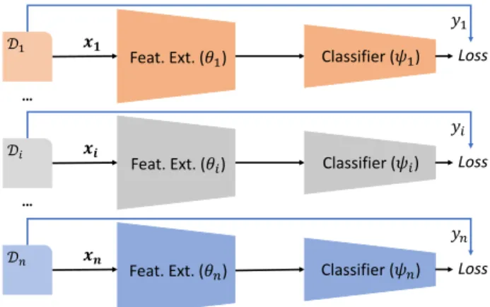
Domain Specific Models Our goal is to improve robustness by exposing individual modules to neighbours that are badly calibrated to a given domain. To obtain these ‘badly calibrated’ components, we also train domain-specific models. As illus-trated in Fig.2, this means that each domainihas its own model composed of feature extractorθiand classifierψi. Each

domain-specific module is only exposed to data of that corresponding domain. To train domain-specific models, we optimise:

argmin [θ1,...,θn],[ψ1,...,ψn] EDi∼D E(xi,yi)∼Di `(yi,ψi(θi(xi)) (2)

Episodic Training Our goal is to train a domain agnostic model, as perψandθin the aggregation method in Eq.1. And we will design an episodic scheme that makes use of the domain-specific modules as per Eq. 2to help the domain-agnostic

2_{At least in the homogeneous case}

Feat. Ext. (!") Classifier (#")

$"

…

Loss %&

'"

Feat. Ext. (!() Classifier (#()

$(

…

Loss

%)

'(

Feat. Ext. (!*) Classifier (#*)

$* %+ _Loss

'*

Figure 2:Illustration of domain-specific branches. One classifier and feature extractor are trained per-domain.

model achieve the desired robustness. Specifically, we will generate episodes where each domain agnostic moduleψandθ

is paired with a domain-specific partner that ismismatchedwith the current data being input. So module and data combinations of the form(ψ,θi,xi0)and(ψ_i,θ,x_i0)wherei6=i0.

3.2. Episodic Training of Feature Extractor

To train a robust feature extractorθ, we ask it to learn features which are robust enough that data from domainican be processed by a classifier that has never experienced domain

ibefore as shown in Fig.3. To generate episodes according to this criterion, we optimise

argmin θ E i,j∼[1,n],i6=j E(xi,yi)∼Di `(yi,ψj(θ(xi)) (3) wherei=6 jandψ_jmeans thatψjis considered constant for the

generation of this loss, i.e., it does not receive back-propagated gradients. This gradient-blocking is important, because without it the dataxifrom domainiwould ‘pollute’ the classifierψj

which we want to retain as being naive to domains outside ofj. Thus in this optimisation, only the feature extractor θ

is penalized whenever the classifier ψj makes the wrong

prediction. That means that, for this loss to be minimised, the shared feature extractorθmust map dataxiinto a format that a

‘naive’ classifierψjcan correctly classify. The feature extractor

must learn to help a classifier recognize a data point that is from a domain that is novel to that classifier.

3.3. Episodic Training of Classifier

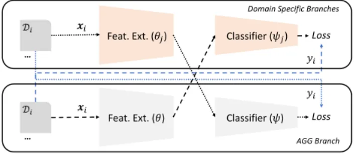
Analogous to the above, we can also interpret DG as the requirement that a classifier should be robust enough to classify data even if it is encoded by a feature extractor which has never seen this type of data in the past, as illustrated in Fig.3. Thus to train the robust classifierψwe ask it to classify domaini

324 325 326 327 328 329 330 331 332 333 334 335 336 337 338 339 340 341 342 343 344 345 346 347 348 349 350 351 352 353 354 355 356 357 358 359 360 361 362 363 364 365 366 367 368 369 370 371 372 373 374 375 376 377 378 379 380 381 382 383 384 385 386 387 388 389 390 391 392 393 394 395 396 397 398 399 400 401 402 403 404 405 406 407 408 409 410 411 412 413 414 415 416 417 418 419 420 421 422 423 424 425 426 427 428 429 430 431 … … !"

Feat. Ext. (#$) Classifier (%$)

&"

Feat. Ext. (#) Classifier (%) Loss

!" &"

Loss

Episodic training of AGG Classifier Episodic training of AGG Feat. Ext.

Domain Specific Branches

AGG Branch

'"

'"

Figure 3: Episodic training for feature and classifier regularisation. The shared feature extractor feeds domain specific classifiers. The shared classifier reads domain-specific feature extractors.

θj. To generate episodes according to this criterion, we do: argmin ψ E i,j∼[1,n],i6=j E(xi,yi)∼Di `(yi,ψ(θj(xi)) (4) where i 6= j and θj means θj is considered constant for

generation of the loss here. Similar to the training of the feature extractor module, this operation is important to retain the domain-specificity of feature extractorθj. The result is that

only the classifierψis penalised, and in order to minimise this lossψmust be robust enough to accept dataxithat has been

encoded by a naive feature extractorθj.

3.4. Episodic Training by Random Classifier

The episodic feature training strategy above is limited to the homogeneous DG setting, since it requires all domains to share label-space in order to create episodes. But in the heterogeneous scenarios, the shared label-space assumption is not met. We next introduce a novel feature training strategy that is suitable for both homogeneous and heterogeneous label-spaces.

In Section 3.2, we introduced the notion of regularising a deep feature extractor by requiring it to support a classifier inexperienced with data from the current domain. Taking this to an extreme, we consider asking the feature extractor to support the predictions of a classifier withrandom weights, as shown in Fig.4. To this end, our objective function here is:

argmin θ E Di∼D E(xi,yi)∼Di `(yi,ψr(θ(xi)) (5) where,ψris a randomly initialised classifier, andψrmeans

it is a constant not updated in the optimization. This can be seen as an extreme version of our earlier episodic cross-domain feature extractor training (not only it has not seen any data from domainxi, but it has not seen any data at all). Moreover, it has

the benefit of not requiring a label-space to be shared across all training domains unlike the previous method in Eq.3.

Specifically, in Eq.3, the routingxi7→θ7→ψjrequiresψj

to have a label-space matching(xi,yj). But for Eq.5, each

domain can be equipped with its own random classifierψrwith

Rand Clf. (!") Loss

# Episodic training by random classifier

$%

Feat. Ext. (&) Classifier (!) $' _$(

…

… Loss

)

#

Aggregate source domains

Figure 4:The architecture of random classifier regularization.

Algorithm 1Episodic Training for Domain Generalization 1: Input:D=[D1,D2,...,Dn]

2: Initialise hyper parameters:λ1,λ2,λ3,α

3: Initialise model parameters: domain specific modules

θ1, ..., θn and ψ1, ..., ψn; AGG modules θ, ψ; random

classifierψr

4: whilenot done trainingdo

5: for(θi,ψi)∈[(θ1,ψ1),...,(θn,ψn)]do 6: Updateθi:=θi−α∇θi(Lds) 7: Updateψi:=ψi−α∇ψi(Lds) 8: end for

9: Updateθ:=θ−α∇θ(Lagg+λ1Lepif+λ3Lepir) 10: Updateψ:=ψ−α∇ψ(Lagg+λ2Lepic)

11: end while

12: Output:θ,ψ

a cardinality matching its normal label-space. This property makes Eq.5suitable for heterogeneous domains.

3.5. Algorithm Flow

Our full algorithm brings together the domain agnostic modules that are our goal to train and the supporting domain-specific modules that help train them (Section3.1). We generate episodes according to the three strategies introduced above. Referring the losses in Eq.1,2,3,4,5asLagg,Lds,Lepif,

Lepic,Lepir, then overall we optimise:

Lfull=Lagg+Lds+λ1Lepif+λ2Lepic+λ3Lepir (6)

for parameters θ, φ,{θi, ψi}ni=1. The full pseudocode for the algorithm is given in Algorithm1. It is noteworthy that, in practice, when training we first warm up the domain-specific branches for a few iterations before training both the domain-specific and domain-agnostic modules jointly.

4. Experiments

4.1. Datasets and Settings

Datasets We evaluate our algorithm on three different homo-geneousDG benchmarks and introduce a novel and larger scale

heterogeneousDG benchmark. The datasets are:IXMAS:[37] is cross-view action recognition task. Two object recognition

432 433 434 435 436 437 438 439 440 441 442 443 444 445 446 447 448 449 450 451 452 453 454 455 456 457 458 459 460 461 462 463 464 465 466 467 468 469 470 471 472 473 474 475 476 477 478 479 480 481 482 483 484 485 486 487 488 489 490 491 492 493 494 495 496 497 498 499 500 501 502 503 504 505 506 507 508 509 510 511 512 513 514 515 516 517 518 519 520 521 522 523 524 525 526 527 528 529 530 531 532 533 534 535 536 537 538 539

benchmarks include:VLCS[8], which includes images from four famous datasets PASCAL VOC2007 (V) [7], LabelMe (L) [31], Caltech (C) [19] and SUN09 (S) [6] and the more recent

PACSwhich has a larger cross-domain gap than VLCS [17]. It contains four domains covering Photo (P), Art Painting (A), Car-toon (C) and Sketch (S) images.VD: For the final benchmark we repurpose the Visual Decathlon [28] benchmark to evaluate DG.

Competitors We evaluate the following competitors:

AGG the vanilla aggregation method, introduced in Eq. 1, trains a single model for all source domains. DICA[26] a kernel-based method for learning domain invariant feature representations.LRE-SVM[38] a SVM-based method, that trains different SVM model for each source domain. For a test domain, it uses the SVM model from the most similar source domain. D-MTAE[12] a de-noising multi-task auto encoder method, which learns domain invariant features by cross-domain reconstruction. DSN [4] Domain Separation Networks decompose the sources domains into shared and private spaces and learns them with a reconstruction signal.

TF-CNN[17] learns a domain-agnostic model by factoring out the common component from a set of domain-specific models, as well as tensor factorization to compress the model parameters.

CCSA[25] uses semantic alignment to regularize the learned feature subspace. DANN [11] Domain Adversarial Neural Networks train a feature extractor with a domain-adversarial loss among the source domains. The source-domain invariant feature extractor is assumed to generalise better to novel target domains. MLDG [18] A recent meta-learning based optimization method. It mimics the DG setting by splitting source domains into meta-train and meta-test, and modifies the optimisation to improve meta-test performance.Fusion[23] A method that fuses the predictions from source domain classifiers for the target domain.MMD-AAE[20] A recent method that learns domain invariant feature autoencoding with adversarial training and ensuring that domains are aligned by the MMD constraint.CrossGrad[32] A recent method that uses Bayesian networks to perturb the input manifold for DG.MetaReg[1] A recent DG method that meta-learns the classifier regularizer. We note that DANN (domain adaptation) is not designed for DG. However, DANN learns domain invariant features, which is natural for DG. And we found it effective for this problem. Therefore we repurpose it as a baseline.

We call our method as Episodic. We useEpi-FCR to denote our full method with (f)eature regularisation, (c)lassifier regularisation and (r)andom classifier regularisation respectively. Ablated variants such asEpi-Fdenote feature regularisation alone, etc. Episodic is implemented using PyTorch.

4.2. Evaluation on

dataset

Settings IXMAS contains 11 different human actions. All actions were video recorded by 5 cameras with different views (referred as 0,...,4). The goal is to train an action recognition model on a set of source views (domains), and recognise the

action from a novel target view (domain). We follow [20] to keep the first 5 actions and use the same Dense trajectory features as input. For our method, we follow [20] to use a one-hidden layer network with 2000 hidden neurons as our backbone and report the average result of 20 runs. The optimizer is M-SGD with learning rate 1e-4, momentum 0.9, weight decay 5e-5. We useλ1=2.0,λ2=2.0, andλ3=0.5.

Results From the results in Table1, we can see that: (i) The vanilla aggregation method, AGG is a strong competitor com-pared to several prior published methods, as is DANN, which is newly identified by us as an effective DG algorithm. (ii) Overall our Epi-FCR performs best, improving 2.4% on AGG, and 1.1% on prior state-of-the-art MMD-AAE. (iii) Particularly in view 1&2 our method achieves new state-of-the art performance.

4.3. Evaluation on

dataset

Settings VLCS domains share 5 categories: bird, car, chair, dog and person. We use pre-extracted DeCAF6 features and follow [25] to randomly split each domain into train (70%) and test (30%) and do leave-one-out evaluation. We use a 2 fully connected layer architecture with output size of 1024 and 128 with ReLU activation, as per [25] and report the average performance of 20 trials. The optimizer is M-SGD with learning rate 1e-3, momentum 0.9 and weight decay 5e-5. We useλ1=5.0,λ2=2.0, andλ3=3.0.

Results From the results in Table2, we can see that: (i) The simple AGG baseline is again competitive with many published alternatives, so is DANN. (ii) Our Epi-FCR method achieves the best performance, improving on AGG by 1.7% and performing comparably to prior state-of-the-art MMD-AAE and MLDG with 0.6% improvement over both.

4.4. Evaluation on

dataset

Settings PACS is a recent dataset with different object style depictions, and a more challenging domain shift than VLCS, as shown in [17]. This dataset shares 7 object categories across domains, including dog, elephant, giraffe, guitar, house, horse and person. We follow the protocol in [17] including the recommended train and validation split for fair comparison. We first follow [17] in using the ImageNet pretrained AlexNet (in Table3) and subsequently also use a modern ImageNet pre-trained ResNet-18 (in Table4) as a base CNN architecture. We train our network using the M-SGD optimizer (batch size/per domain=32, lr=1e-3, momentum=0.9, weight decay=5e-5) for 45k iterations when using AlexNet and train our network using same optimizer (weight decay=1e-4) for ResNet-18. We use

λ1=2.0,λ2=0.05, andλ3=0.1 for both settings. We use the official PACS protocol and split [17] and rerun MetaReg [1] on this split, since MetaReg did not release their protocol.

Results From the AlexNet results in Table3, we can see that: (i) Our episodic method obtained the best performance on held out domains C and S and comparable performance

540 541 542 543 544 545 546 547 548 549 550 551 552 553 554 555 556 557 558 559 560 561 562 563 564 565 566 567 568 569 570 571 572 573 574 575 576 577 578 579 580 581 582 583 584 585 586 587 588 589 590 591 592 593 594 595 596 597 598 599 600 601 602 603 604 605 606 607 608 609 610 611 612 613 614 615 616 617 618 619 620 621 622 623 624 625 626 627 628 629 630 631 632 633 634 635 636 637 638 639 640 641 642 643 644 645 646 647

Source Target DICA [26] LRE-SVM [38] D-MTAE [12] CCSA [25] MMD-AAE [20] DANN[11] MLDG [18] CrossGrad [32] MetaReg [1] AGG Epi-FCR

0,1,2,3 4 61.5 75.8 78.0 75.8 79.1 75.0 70.7 71.6 74.2 73.1 76.9 0,1,2,4 3 72.5 86.9 92.3 92.3 94.5 94.1 93.6 93.8 94.0 94.2 94.8 0,1,3,4 2 74.7 84.5 91.2 94.5 95.6 97.3 97.5 95.7 96.9 95.7 99.0 0,2,3,4 1 67.0 83.4 90.1 91.2 93.4 95.4 95.4 94.2 97.0 95.7 98.0 1,2,3,4 0 71.4 92.3 93.4 96.7 96.7 95.7 93.6 94.0 94.7 94.4 96.3 Ave. 69.4 84.6 87.0 90.1 91.9 91.5 90.2 89.9 91.4 90.6 93.0

Table 1:Cross-view action recognition results (accuracy. %) on IXMAS dataset.

Source Target DICA [26] LRE-SVM [38] D-MTAE [12] CCSA [25] MMD-AAE[20] DANN [11] MLDG [18] CrossGrad [32] MetaReg[1] AGG Epi-FCR

L,C,S V 63.7 60.6 63.9 67.1 67.7 66.4 67.7 65.5 65.0 65.4 67.1

V,C,S L 58.2 59.7 60.1 62.1 62.6 64.0 61.3 60.0 60.2 60.6 64.3

V,L,S C 79.7 88.1 89.1 92.3 94.4 92.6 94.4 92.0 92.3 93.1 94.1

V,L,C S 61.0 54.9 61.3 59.1 64.4 63.6 65.9 64.7 64.2 65.8 65.9

Ave. 65.7 65.8 68.6 70.2 72.3 71.7 72.3 70.5 70.4 71.2 72.9

Table 2:Cross-dataset object recognition results (accuracy. %) on VLCS benchmark.

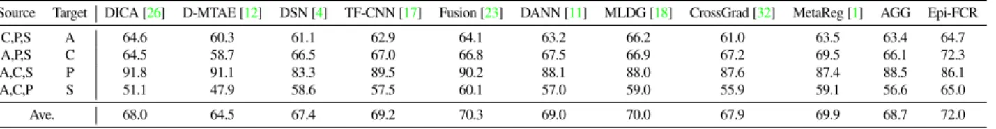
Source Target DICA [26] D-MTAE [12] DSN [4] TF-CNN [17] Fusion [23] DANN [11] MLDG [18] CrossGrad [32] MetaReg [1] AGG Epi-FCR

C,P,S A 64.6 60.3 61.1 62.9 64.1 63.2 66.2 61.0 63.5 63.4 64.7

A,P,S C 64.5 58.7 66.5 67.0 66.8 67.5 66.9 67.2 69.5 66.1 72.3

A,C,S P 91.8 91.1 83.3 89.5 90.2 88.1 88.0 87.6 87.4 88.5 86.1

A,C,P S 51.1 47.9 58.6 57.5 60.1 57.0 59.0 55.9 59.1 56.6 65.0

Ave. 68.0 64.5 67.4 69.2 70.3 69.0 70.0 67.9 69.9 68.7 72.0

Table 3:Cross-domain object recognition results (accuracy. %) of different methods on PACS using pretrained AlexNet.

Source Target AGG DANN [11] MLDG [18] CrossGrad [32] MetaReg [1] Epi-FCR

C,P,S A 77.6 81.3 79.5 78.7 79.5 82.1

A,P,S C 73.9 73.8 77.3 73.3 75.4 77.0

A,C,S P 94.4 94.0 94.3 94.0 94.3 93.9

A,C,P S 70.3 74.3 71.5 65.1 72.2 73.0

Ave. 79.1 80.8 80.7 77.8 80.4 81.5

Table 4:Cross-domain object recognition results (accuracy. %) of different methods on PACS using ResNet-18.

on A, P domains. (ii) It also achieves the best performance overall, with 3.3% improvement on vanilla AGG, and at least 1.7% improvement on prior state-of-the-art methods MLDG [18], Fusion [23] and MetaReg [1].

Meanwhile in Table4, we see that with a modern ResNet-18 architecture, the basic results are improved across the board as expected. However our full episodic method maintains the best performance overall, with a 2.4% improvement on AGG.

We note here that when using modern architectures like

[34, 13] for DG tasks we need to be careful with batch

normalization [14]. Batchnorm accumulates statistics of the training data during training, for use at testing. In DG, the source and target domains have domain-shift between them, so different ways of employing batch norm produce different results. We tried two ways of coping with batch norm, one is directly using frozen pre-trained ImageNet statistics. Another is to unfreeze and accumulate statistics from the source domains. We observed that when training ResNet-18 on PACS with accu-mulating the statistics from source domains it produced a worse accuracy than freezing ImageNet statistics (75.7%vs79.1%).

A->S A->C C->A C->S S->C S->A AGG feat. ext. 0.4 0.5 0.6 0.7 0.8 0.9 1.0 Test accuracy w Episodic w/o Episodic

A->S A->C C->A C->S S->C S->A AGG classifier 0.4 0.5 0.6 0.7 0.8 0.9 1.0 Test accuracy w Episodic w/o Episodic

Figure 5:Cross-domain test accuracy with shared feature extractor or classifier. A7→C means, feed A data through C-specific module. Eg, left:xA7→θ7→ψC, right:xA7→θC7→ψ. Higher is better.

4.5. Further Analysis and Insights

Ablation Study To understand the contribution of each component of our model, we perform an ablation study using PACS-AlexNet shown in Fig. 6a. Episodic training for the feature extractor, gives a 1.6% boost over the vanilla AGG. In-cluding episodic training of the classifier, further improves 0.5%. Finally, combine all the episodic training components, provides 3.3% improvement over vanilla AGG. This confirms that each component of our model contributes to final performance.

Cross-Domain Testing Analysis To understand how our Epi-FCR method obtains its improved robustness to domain shift, we study its impact on cross-domain testing. Recall that when we activate the episodic training of the agnostic feature extractor and classifier, we benefit from the domain specific branches by routing domainidata across domainj

branches. E.g., we feed:xi7→θ7→ψj7→yito train Eq.3, and

xi7→θj7→ψ7→yito train Eq.4.

648 649 650 651 652 653 654 655 656 657 658 659 660 661 662 663 664 665 666 667 668 669 670 671 672 673 674 675 676 677 678 679 680 681 682 683 684 685 686 687 688 689 690 691 692 693 694 695 696 697 698 699 700 701 702 703 704 705 706 707 708 709 710 711 712 713 714 715 716 717 718 719 720 721 722 723 724 725 726 727 728 729 730 731 732 733 734 735 736 737 738 739 740 741 742 743 744 745 746 747 748 749 750 751 752 753 754 755

training the models. As illustrated in Fig.53, we can see that the episodic training strategy indeed improves cross-domain testing performance. For example, when we feed domainAdata to domainCclassifierxA7→θ7→ψC7→yA, the Episodic-trained

agnostic extractorθimproves the performance of the domain-C classifier who has never experienced domain A data (Fig.5, left); and similarly for the Episodic-trained agnostic classifier.

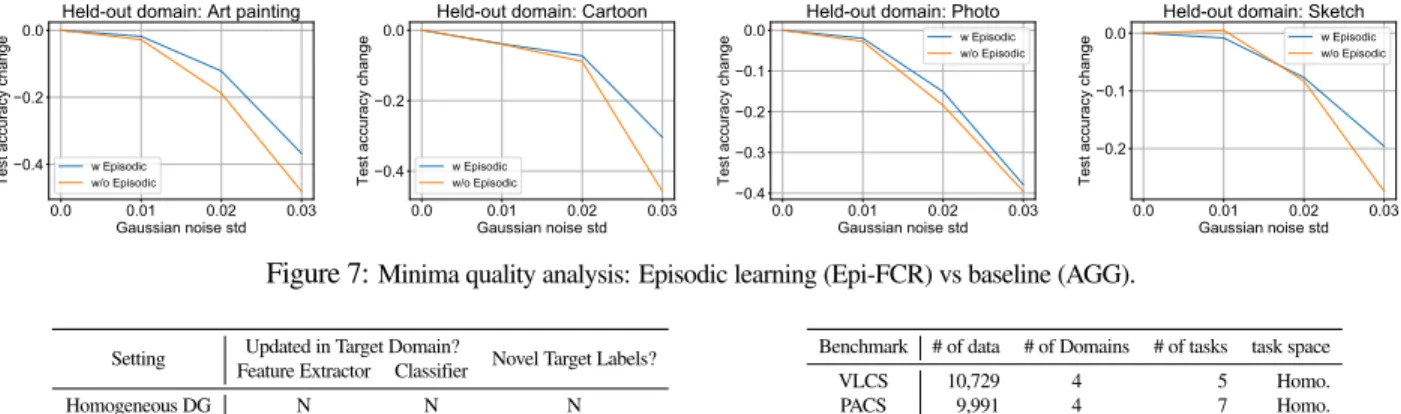
Analysis of Solution Robustness In the above experiments we confirmed that our episodic model outperforms the strong AGG baseline in a variety of benchmarks, and that each component of our framework contributes. In terms of analysing the mechanism by which episodic training improves robustness to domain shift, one possible route is through leading the model to find a higher quality minima. Several studies recently have analysed learning algorithm variants in terms of the quality of the minima that they leads a model to [15,5].

One intuition is that converging to a ‘wide’ rather than ‘sharp’ minima provides a more robust solution, because perturbations (such as domain shift, in our case) are less likely to cause a big hit to accuracy if the model’s performance is not dependent on a very precisely calibrated solution. Following [15,40], we therefore compare the solutions found by AGG and our Epi-FCR by adding noise to the weights of the converged model, and observing how quickly the testing accuracy decreases with the magnitude of the noise. From Fig.7we can see that both models’ performance drops as weights are perturbed, but our Epi-FCR model is more robust to weight perturbations. This suggests that the minima found by Epi-FCR is a more robust one than that found by AGG, which may explain the improved cross domain robustness of Epi-FCR compared to AGG.

Computational Cost Our Episodic model is comparable in cost overall to many contemporaries. Our Epi-C variant does re-quire training multiple feature extractors for the source domains (as do [16,38,17,23]). However, users are more practically in-terested in testing performance, where our model is as small, fast and simple as AGG (unlike, e.g., [38,23]). In terms of training requirements, we note that only the Epi-C variant requires multi-ple feature extractor training, so Epi-FR can still safely be used if this is an issue. Furthermore if a large number of source domains are present, we can sample a subset of them at each batch.

Concretely, we compare the training time of different methods in Fig. 6b. All the methods were run on PACS (ResNet-18) for 3k iterations with CPU: Intel i7-7820 (@3.60GHz x 16) and GPU: 1080Ti. As expected vanilla AGG is the fastest to train (9.8 mins), so we regard it as the the base unit. The second tier are our Epi-F and Epi-R. As expected without Epi-C, our Epi-F and Epi-R variants run fast. The next tier are MetaReg, Epi-FCR and MLDG. And the most expensive one is CrossGrad. Although the use of ‘Epi-C’ here requires domain-specific feature extractors, our Epi-FCR is still 3_{To save space we only display the leave-photo-out split. The others are}

consistent with these observations.

A C P S Ave. 0.6 0.7 0.8 0.9 Accuracy AGG Epi-F Epi-FC Epi-FCR (a) 0 2 4 6 8 10 12 14 Time AGG MLDG CrossGrad MetaReg Epi-FCR Epi-C Epi-F Epi-R (b)

Figure 6: (a) Ablation study on PACS (↑). (b) Computational cost comparison on PACS (↓).

comparably efficient. This is because our episodic training does not generate multi-step graph unrolling or meta-optimization in gradient updates. As a result, our time cost is on par with MetaReg [1] and faster than MLDG [18] and CrossGrad [32].

4.6. Evaluation on

dataset

Heterogeneous Problem Setting Visual Decathlon contains ten datasets and was initially proposed as a multi-domain learn-ing benchmark [28]. We re-purpose Decathlon for a more am-bitious challenge of domain generalisation. As explained earlier, our motivation is find out if DG learning can improve thedefacto

standard ‘ImageNet trained CNN feature extractor’ for use as a fixed off-the-shelf representation for new target problems. In this case the feature extractor is trained on the source domain, and used to extract features of the target domain data. Then a target domain-specific classifier (we use SVM) is trained to classify in the target domain. As explained in Table5(left), this is quite dif-ferent from the standard DG setting in that target domain labels

areused (for shallowclassifiertraining), but the focus here is on the robustness of the learned feature when generalising to repre-sentnew domains and tasks without further fine-tuning. If DG training can improve feature generalisation compared to a vanilla ImageNet CNN, this could be of major practical value given the widespread usage of this workflow by vision practitioners.

Besides evaluating a potentially more generally useful prob-lem setting compared to standard homogeneous DG, our VD experiment is also a larger scale evaluation compared to existing DG studies. As shown in Table5(right), VD-DG has twice the domains of VLCS and PACS and is an order of magnitude larger evaluation in terms of data and category numbers.

Settings We consider the five largest datasets in VD (CIFAR-100, Daimler Ped, GTSRB, Omniglot and SVHN, excluding Im-ageNet4) as our source domains, and the four smallest datasets (Aircraft, D. Textures, VGG-Flowers and UCF101) as our target domains. The goal is to use DG training among the five datasets to learn a feature which outperforms the off-the-shelf ImageNet-trained CNN that we use as an initial condition. We use ResNet-18 [13] as the backbone model, and resize all the images to 64x64 for computational efficiency. To support the VD hetero-geneous label space, we assume a shared feature extractor, and

4_{We always exploit ImageNet as an initial condition, but do not include}

756 757 758 759 760 761 762 763 764 765 766 767 768 769 770 771 772 773 774 775 776 777 778 779 780 781 782 783 784 785 786 787 788 789 790 791 792 793 794 795 796 797 798 799 800 801 802 803 804 805 806 807 808 809 810 811 812 813 814 815 816 817 818 819 820 821 822 823 824 825 826 827 828 829 830 831 832 833 834 835 836 837 838 839 840 841 842 843 844 845 846 847 848 849 850 851 852 853 854 855 856 857 858 859 860 861 862 863 0.0 0.01 0.02 0.03 Gaussian noise std 0.4 0.2 0.0

Test accuracy change

Held-out domain: Art painting

w Episodic w/o Episodic 0.0 0.01 0.02 0.03 Gaussian noise std 0.4 0.2 0.0

Test accuracy change

Held-out domain: Cartoon

w Episodic w/o Episodic 0.0 0.01 0.02 0.03 Gaussian noise std 0.4 0.3 0.2 0.1 0.0

Test accuracy change

Held-out domain: Photo

w Episodic w/o Episodic 0.0 0.01 0.02 0.03 Gaussian noise std 0.2 0.1 0.0

Test accuracy change

Held-out domain: Sketch

w Episodic w/o Episodic

Figure 7:Minima quality analysis: Episodic learning (Epi-FCR) vs baseline (AGG).

Setting Updated in Target Domain? Novel Target Labels? Feature Extractor Classifier

Homogeneous DG N N N

Heterogeneous DG N Y Y

Benchmark # of data # of Domains # of tasks task space

VLCS 10,729 4 5 Homo.

PACS 9,991 4 7 Homo.

VD-DG 238,215 9 2128 Hetero.

Table 5:Left: Difference between conventional homogeneous DG setting and new heterogeneous DG setting. Right: Contrasting the larger scale of our VD-DG (excluding ImageNet) vs previous DG benchmarks.

Target ImageNet PT AGG DANN [11] MLDG [18] CrossGrad [32] Epi-R

Concate Mean Concate Mean Concate Mean Concate Mean Concate Mean

Aircraft 12.7 17.4 14.6 17.4 15.0 17.4 14.2 17.2 13.7 17.7 13.9 D. Textures 35.2 37.7 35.1 37.9 36.6 38.3 34.6 34.6 31.4 40.2 37.8 VGG-Flowers 48.1 56.3 52.0 55.5 52.2 54.0 53.2 49.2 49.3 55.4 53.0 UCF101 35.0 43.3 35.0 44.5 36.1 44.4 36.7 42.7 35.7 45.7 37.1 Ave. 32.8 38.7 34.2 38.8 35.0 38.5 34.7 35.9 32.5 39.7 35.5 VD-Score 185 265 185 277 202 279 194 241 169 304 217

Table 6:Results of top-1 accuracy (%) and visual decathlon overall scores of different methods on VD-DG. Train on CIFAR-100, Daimler Ped, GTSRB, Omniglot, SVHN and test on Aircraft, D. Textures, VGG-Flowers, UCF101.

a source domain-specific classifier. We perform episodic DG training among the source domains, using our (R)andom clas-sifier model variant, which supports heterogeneous label-spaces. After DG training, the model will then be used as a fixed feature extractor for the held out target domain. These are combined by combination (concatenation and mean-pooling) with the original ImageNet pre-trained features5_{. This final feature is used to train} a linear SVM for the corresponding task, as per common prac-tice. We train the network using the M-SGD optimizer (batch size/per domain=32, lr=1e-3, momentum=0.9, weight decay=1e-4) for 100k iterations where the lr is decayed in 40k, 80k iter-ations by a factor 10. We setλ3=_t+502.5 ,tis the iteration num.

Results From the results in Table6, we observed that: (i) We do learn a feature that is more robust to novel domains compared to the standard ImageNet pre-trained features (Epi-R vs ImageNetPT improves 7.1% or 2.7% on held-out datasets). However this is not very surprising as we use more data than this baseline. (ii) The vanilla AGG method provides a direct and fair comparison, as it also exploits this additional data to improve on the ImageNetPT baseline. Our Epi-R provides a clear improvement on AGG, demonstrating the value of our proposed Episodic training scheme. (iii) In terms of other DG competitors: we note that besides MLDG [18] and CrossGrad [32], the only 5_{Since ImageNet is excluded from source domains for computational}

feasibility, there is loss of performance for all models compared to the original feature due to the forgetting effect.

other competitor that we were able to feasibly run on this large scale benchmark was DANN – method that we first identified as re-purposeable for DG in this paper. Other methods either do not support heterogeneous label-spaces or, do not scale to this many domains, or this many examples. (iv) Overall our Epi-R method outperforms all alternatives in both average accuracy, and also the VD score recommended in preference to accuracy in [28]. Overall this is the first demonstration that any DG method can improve robustness to domain shift in a larger-scale setting, across heterogeneous domains, and make a practical impact in surpassing ImageNet feature performance.

5. Conclusion

In this paper, we addressed the domain generalisation problem. We proposed a simple episodic training strategy that mimics train-test domain-shift scenario during training, thus improving the trained model’s robustness to novel domains. We showed that our method achieves state-of-the-art performance on all the main existing DG benchmarks. We also performed the largest DG evaluation to date, using the Visual Decathlon benchmark. Importantly, we provided the first demonstration of DG’s potential value ‘in the wild’ – by demonstrating our model’s potential to improve the performance of thedefacto

standard ImageNet pre-trained CNN as a fixed feature extractor for novel downstream problems.

864 865 866 867 868 869 870 871 872 873 874 875 876 877 878 879 880 881 882 883 884 885 886 887 888 889 890 891 892 893 894 895 896 897 898 899 900 901 902 903 904 905 906 907 908 909 910 911 912 913 914 915 916 917 918 919 920 921 922 923 924 925 926 927 928 929 930 931 932 933 934 935 936 937 938 939 940 941 942 943 944 945 946 947 948 949 950 951 952 953 954 955 956 957 958 959 960 961 962 963 964 965 966 967 968 969 970 971

References

[1] Y. Balaji, S. Sankaranarayanan, and R. Chellappa. Metareg: Towards domain generalization using meta-regularization. In

NeurIPS, 2018.5,6,7

[2] S. Ben-David, J. Blitzer, K. Crammer, and F. Pereira. Analysis of representations for domain adaptation. InNIPS, 2006.1

[3] H. Bilen and A. Vedaldi. Universal representations: The missing link between faces, text, planktons, and cat breeds. Technical report, 2017.2

[4] K. Bousmalis, G. Trigeorgis, N. Silberman, D. Krishnan, and D. Erhan. Domain separation networks. InNIPS, 2016.1,5,6

[5] P. Chaudhar, A. Choromansk, S. Soatt, Y. LeCun, C. Baldass, C. Borg, J. Chays, L. Sagun, and R. Zecchina. Entropy-sgd: Biasing gradient descent into wide valleys. InICLR, 2017.7

[6] M. J. Choi, J. Lim, and A. Torralba. Exploiting hierarchical context on a large database of object categories. InCVPR, 2010.5

[7] M. Everingham, L. Van Gool, C. K. I. Williams, J. Winn, and A. Zisserman. The pascal visual object classes (voc) challenge.

IJCV, 2010.5

[8] C. Fang, Y. Xu, and D. N. Rockmore. Unbiased metric learning: On the utilization of multiple datasets and web images for softening bias. InICCV, 2013.5

[9] C. Finn, P. Abbeel, and S. Levine. Model-agnostic meta-learning for fast adaptation of deep networks. InICML, 2017.1,2

[10] Y. Ganin and V. Lempitsky. Unsupervised domain adaptation by backpropagation. InICML, 2015.1

[11] Y. Ganin, E. Ustinova, H. Ajakan, P. Germain, H. Larochelle, F. Laviolette, M. Marchand, and V. Lempitsky. Domain-adversarial training of neural networks. JMLR, 2016.5,6,8

[12] M. Ghifary, W. B. Kleijn, M. Zhang, and D. Balduzzi. Domain generalization for object recognition with multi-task autoencoders. InICCV, 2015.1,2,5,6

[13] K. He, X. Zhang, S. Ren, and J. Sun. Deep residual learning for image recognition. InCVPR, 2016.6,7

[14] S. Ioffe and C. Szegedy. Batch normalization: Accelerating deep network training by reducing internal covariate shift. InICML, 2015.6

[15] N. S. Keskar, D. Mudigere, J. Nocedal, M. Smelyanskiy, and P. T. P. Tang. On large-batch training for deep learning: Generalization gap and sharp minima. InICLR, 2017.7

[16] A. Khosla, T. Zhou, T. Malisiewicz, A. Efros, and A. Torralba. Undoing the damage of dataset bias. InECCV, 2012.1,2,7

[17] D. Li, Y. Yang, Y.-Z. Song, and T. Hospedales. Deeper, broader and artier domain generalization. InICCV, 2017.1,2,3,5,6,7

[18] D. Li, Y. Yang, Y.-Z. Song, and T. Hospedales. Learning to generalize: Meta-learning for domain generalization. InAAAI, 2018.1,2,5,6,7,8

[19] F.-F. Li, F. Rob, and P. Pietro. Learning generative visual models from few training examples: an incremental bayesian approach tested on 101 object categories. InCVPR Workshop

on Generative-Model Based Vision, 2004.5

[20] H. Li, S. Jialin Pan, S. Wang, and A. C. Kot. Domain generaliza-tion with adversarial feature learning. InCVPR, 2018.2,5,6

[21] M. Long, Y. Cao, J. Wang, and M. Jordan. Learning transferable features with deep adaptation networks. InICML, 2015.1

[22] M. Long, H. Zhu, J. Wang, and M. I. Jordan. Unsupervised do-main adaptation with residual transfer networks. InNIPS, 2016.1

[23] M. Mancini, S. R. Bulo‘, B. Caputo, and E. Ricci. Best sources forward: Domain generalization through source-specific nets. In

ICIP, 2018.5,6,7

[24] N. Mishra, M. Rohaninejad, X. Chen, and P. Abbeel. Meta-learning with temporal convolutions. arXiv, 2017.2

[25] S. Motiian, M. Piccirilli, D. A. Adjeroh, and G. Doretto. Unified deep supervised domain adaptation and generalization. InICCV, 2017.5,6

[26] K. Muandet, D. Balduzzi, and B. Sch¨olkopf. Domain generaliza-tion via invariant feature representageneraliza-tion. InICML, 2013.1,2,5,6

[27] S. Ravi and H. Larochelle. Optimization as a model for few-shot learning. InICLR, 2017.1,2

[28] S.-A. Rebuffi, H. Bilen, and A. Vedaldi. Learning multiple visual domains with residual adapters. InNIPS, 2017.2,5,7,8

[29] S.-A. Rebuffi, H. Bilen, and A. Vedaldi. Efficient parametrization of multi-domain deep neural networks. InCVPR, 2018.2

[30] O. Russakovsky, J. Deng, H. Su, J. Krause, S. Satheesh, S. Ma, Z. Huang, A. Karpathy, A. Khosla, M. Bernstein, A. C. Berg, and L. Fei-Fei. Imagenet large scale visual recognition challenge.

IJCV, 2015.2

[31] B. Russell, A. Torralba, K. Murphy, and W. Freeman. Labelme: A database and web-based tool for image annotation.IJCV, 2008.5

[32] S. Shankar, V. Piratla, S. Chakrabarti, S. Chaudhuri, P. Jyothi, and S. Sarawagi. Generalizing across domains via cross-gradient training. InICLR, 2018.1,2,5,6,7,8

[33] J. Snell, K. Swersky, and R. S. Zemel. Prototypical networks for few shot learning. InNIPS, 2017.1,2

[34] C. Szegedy, V. Vanhoucke, S. Ioffe, J. Shlens, and Z. Wojna. Rethinking the inception architecture for computer vision. In

CVPR, 2016.6

[35] E. Tzeng, J. Hoffman, N. Zhang, K. Saenko, and T. Darrell. Deep domain confusion: Maximizing for domain invariance.

arXiv, 2014.1

[36] R. Volpi, H. Namkoong, O. Sener, J. Duchi, V. Murino, and S. Savarese. Generalizing to unseen domains via adversarial data augmentation. InNeurIPS, 2018.2

[37] D. Weinland, R. Ronfard, and E. Boyer. Free viewpoint action recognition using motion history volumes. CVIU, 2006.4

[38] Z. Xu, W. Li, L. Niu, and D. Xu. Exploiting low-rank structure from latent domains for domain generalization. InECCV, 2014.

1,5,6,7

[39] Y. Yang and T. M. Hospedales. A unified perspective on multi-domain and multi-task learning. InICLR, 2015.2

[40] Y. Zhang, T. Xiang, T. M. Hospedales, and H. Lu. Deep mutual learning. InCVPR, 2018.7