Model Embedded Control: A Method to Rapidly Synthesize
Control-lers in a Modeling Environment
E. D. Tate Michael Sasena† Jesse Gohl† Michael Tiller†
Hybrid Powertrain Engineering, General Motors Corp.
1870 Troy Tech Park, Troy, Michigan, 48009
†Emmeskay, Inc, 47119 Five Mile Road
Plymouth, Michigan, 48170
[email protected] [email protected] [email protected] [email protected]
Abstract
One of the challenges in modeling complex systems is the creation of quality controllers. In some projects, the effort to develop even a reasonable pro-totype controller dwarfs the effort required to de-velop a physical model. For a limited class of prob-lems, it is possible and tractable to directly synthe-size a controller from a mathematical statement of control objectives and a model of the plant. To do this, a system model is decomposed into a controls model and a plant model. The controls model is fur-ther decomposed into an optimization problem and a ‘zero-time’ plant model. The zero-time plant model in the controller is a copy or a reasonable representa-tion of the real plant model. It is used to evaluate the future impact of possible control actions. This type of controller is referred to as a Model Embedded Controller (MEC) and can be used to realize control-lers designed using Dynamic Programming (DP).
To illustrate this approach, an approximation to the problem of starting an engine is considered. In this problem, an electric machine with a flywheel is connected to crank and slider with a spring attached to the slider. The machine torque is constrained to a value which is insufficient to statically overcome the force of the spring. This constraint prevents the mo-tor from achieving the desired speed from some ini-tial conditions if it only supplies maximal torque in the desired direction of rotation. By using DP, a con-trol strategy that achieves the desired speed from any initial condition is generated. This controller is real-ized in the model using MEC.
The controller for this example is created by forming an optimization problem and calling an em-bedded copy of the plant model. Furthermore, this controller is calibrated by conducting a large scale Design of Experiments (DOE). The experiments are processed to generate the calibrations for the control-ler such that it achieves its design objectives when used for closed loop control of the plant model.
It is well understood that Modelica includes many language features that allow plant models to be developed quickly. As discussed previously, the de-velopment of quality control strategies generally re-mains a bottleneck. In this paper we show how ex-isting features along with appropriate tool support and potential language changes can make a signifi-cant impact on the model development process by supporting an automated control synthesis process. Keywords: Control, Dynamic Programming, Model Embedded Control, Model Based Control, Optimal Control
1 Introduction
The use of modeling is well established in the development of complex products. Modern tools have significantly reduced the effort required to model and tune physical systems. Acausal or topo-logical modeling reduces the effort required to model a system’s physics. The use of optimization allows systematic tuning of parameters to improve a design. The combination of parameter optimization and
rapid modeling allows a large set of potential designs to be quickly evaluated. However for systems which include controls, the development is, in general, a man-power intensive process subject to large uncer-tainty in development time and optimality. The op-timization of both controls and design must be solved in many problems [1-3]. One way to address this problem is to use numerical techniques to con-struct controllers. For certain classes of problems, tractable numerical techniques can be used to de-velop an approximately minimizing controller [4]. A minimizing controller is a controller which achieves the best possible performance from a system as measured against an objective. There may exist more than one controller able to achieve this minimum, but no controller can perform better than a minimiz-ing controller. For this work, the terms minimizminimiz-ing controller and optimal controller are used inter-changeably.
To construct a minimizing controller, an ob-ject cost,
J
, is defined. This is a function which maps the state and input trajectory of the system to a scalar:u
x
C
J
,
.
(1)
Consider the special case of a plant described by or-dinary differential equations with inputs that are piecewise constant. These piecewise constant inputs are updated periodically at the ‘decision instances’ by a controller at intervals of
t
. The total operating cost is calculated as a sum over an infinite time hori-zon. Furthermore, the sum of costs is discounted by the term which is greater than zero and less than or equal to one. The total cost is calculated by an additive function that operates on the instantaneous state and the control inputs. This cost may take a form similar to 1 00
,
k k t k cont k k t tJ x
c
x
u
d
. (2)
The total cost in (2) is a function of the initial state of the system. To simplify notation, let the state at the decision instances be represented by
k k
x
x t
.
(3)
Let the discrete time samples occur at
k
t
k
t
.
(4)
Furthermore, let the continuous-time instantaneous cost,
c
cont, in (2) be represented in discrete time no-tation as an additive cost over an interval,1
,
,
k k t k k cont k t tc x u
c
x
u
d
.
(5)
Using the notation developed in (2) through (5), the continuous-time system’s total cost is expressed in discrete time notation as
0 0
,
k k k kJ x
c x u
.
(6)
To simplify the continuous-time dynamics, let
0
,
,
,
0
t df x u
f
u d
x
. (7)
Hence, 1,
k d k kx
f x u
.
(8)
An optimal control choice for each time step can be found using the dynamic programming equations,
*
arg min
,
,
d u U x
u x
c x u
V f x u
. (9)
The function
V x
is known as the value function. By using the dynamic programming (DP) equations to find the value function, a minimizing controller is obtained. The DP equations aremin
,
d,
u U xV x
c x u
V f x u
, (10)
where,
0
U x
u g x u
(11)
defines the set of feasible actions,
U
x
. For the case where the total cost is considered over an infi-nite horizon andu
ku x
* k (see eq (9)), the value function is the same as the total cost function,x
V
x
J
. Equation (10) can be solved through value iteration, policy iteration, or linear program-ming. See [5-23] for discussion of solution methods. For discussion of using DP to find value functions for automotive control application, see [24-29]. The formulation of equation (11) is chosen to simplify management of constraints throughout the model and to conform to a standard form used in the optimiza-tion community, the negative null form [30].One problem with solving (10) is that when the state space consists of continuous states,
V x
is a function from one infinite set to another. Except in special cases, this requires approximation to solve. One common approach is to use linear bases to ap-proximate the value function. Possible linear bases include the bases for multi-linear interpolation, the bases for barycentric interpolation, b-splines, and polynomials. See the appendices in [25] for a discus-sion of linear bases for dynamic programming. In the case where
V x
is approximated by a linear basis,T
V x
x w
,
(12)
where
1 2 N
x f x f x f x
.
(13)
An approximate solution to (10) is found by finding the weights,
w
, which solvemin , ,
T T
d u U x
x w c x u f x u w
. (14)
See [5-7] for a discussion of using linear bases to form the value function.It is important to understand that this con-troller is an optimal concon-troller for the discrete time case only, when the controller updates every
t
seconds. In other uses, the controller will generally be suboptimal. Additionally, any development algo-rithm based on this methodology will suffer from the curse of dimensionality [31]. In other words, the time to find an optimal controller will increase geo-metrically with the size of the plant state space. As a point of reference, using a single commercially available PC from 2005, a five state controller was found in less than twenty four hours.
2 Controller Development
To use equations (2) through (14) to develop a controller, it is necessary to have a plant model which includes the dynamics (
f
), cost function (c
), and constraints (g
) all coupled to an integrator which can be invoked as a function call by a Control Design Algorithm (CDA). In addition, the set of states for the plant model and the set of controller actions must be specified to the CDA. For this work, a custom wrapper was developed that allowed batches of states and actions to be efficiently evalu-ated. Each evaluation returned the state at the next interval, the cost of operation for the interval, and the constraint activity over the interval.To understand the structure of the equations involved in this work, consider a system consisting of a plant and a controller. Without loss of general-ity, assume the plant dynamics are described by or-dinary differential equations
,
x
f x u
,
(15)
where
f
is a function that describes the plant dy-namics. For notational simplicity consider a continu-ous time controller. Let the controller be a full state feedback controller implemented as a static mapping,M
, from the state,x
, to the action set,u
:u M x
.
(16)
Assuming only a single global minimum exists, the dynamic programming equations in (9) can be di-rectly used for the static mapping (16). The autono-mous dynamics of this system are then described by the following equation
,arg min , d ,
u U x
x f x c x u V f x u
(17)
This equation is then integrated to solve for
x t
,0 , ,arg min , t u U x d x t c x s u f x s ds V f x s u
(18)
where 00
x
x
(19)
defines the initial conditions. To evaluate
f
d from (7), a nested integrator, which is independent of the primary simulation integrator, is required. This nested integrator executes in ‘zero-time’ from the perspective of the primary integrator. We refer to this as an embedded or nested simulation. Because the nested integrator is used inside a numeric optimi-zation, it will potentially be called multiple times at each primary integrator evaluation. Iff
d in (18) is expanded using (7), the plant dynamics function,f
, from (15) occurs in two locations in0 0 , , arg min , , 0 t t u U x x t c x s u f x s ds V f u d x s
(20)
where 00
x
x
(21)
The nested copy of the plant dynamics equations,
f
, is referred to as the embedded or nested model. In the case where the controller is modeled as updating periodically, rather than continuously, the solution to the optimization problem is held constant between controller updates.The equation structure in (20) and the reuse of the plant dynamics function,
f
, offer the ability to quickly synthesize controllers using numerical techniques. However, existing tools make the im-plementation of this type of model problematic. There are two primary issues in implementation. The first is execution efficiency. Few commercial tools have been developed with the goal of efficiently solving this class of equations. Secondly, severalcommercial modeling environments make the defini-tion and reuse of the plant model cumbersome, re-quiring significant efforts during development and maintenance. Fortunately, the features of Modelica make the definition and reuse of a plant model man-ageable. The examples that follow have been devel-oped in Dymola ®, however this general approach has also been used with Simulink® and AMESim®.
To systematically generate a system with an optimal controller, a model of the plant is generated. This plant model is ‘wrapped’ with an application programming interface (API) so a control design al-gorithm can determine the state space, the action space, the state at the next time step, the constraint activity, and the cost for a given state and action. This interaction between the plant model, the API and the control design algorithm is illustrated in Figure 1. The CDA queries the API to determine the structure of the state and action space. Given this structure and the configuration of the CDA, a se-quence of DOEs is executed. The DOE data are used to find a solution to (10). For this work, the value function was modeled using multi-linear interpola-tion and a soluinterpola-tion to (14) was found. To simplify coding, value iteration was used [5, 6] to find
V x
.Control Design Algorithm
Plant Model u x, u x fd , u x g , x V
API to expose functions
u x c , (CDA) State Space Action Space
Figure 1 - Plant Model API
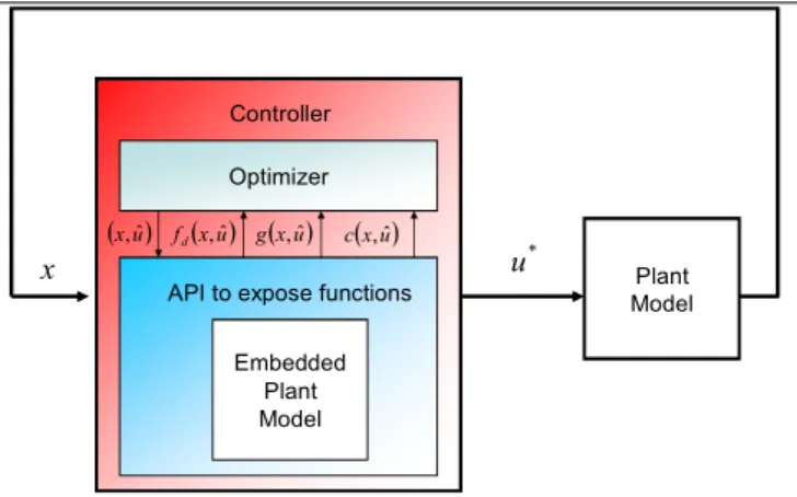
Once the value function is generated, the system model is formed by one of two methods. The first method is by generating a lookup table that maps the state variables to an action as in (16). The process of generating a value function, finding a mapping equivalent to (9), and realizing a controller as a mapping (or lookup table) is referred to as Indi-rect Model Embedded Control (IMEC). This method is appropriate for some systems. Another approach, which is more computationally expensive, is referred to as Direct Model Embedded Control (DMEC). For DMEC, the controller is realized by forming an op-timization statement around an embedded copy of
the plant model. This structure is illustrated in Figure 2. Embedded Plant Model u x,ˆ fdx,uˆ gx,uˆ
API to expose functions Controller Plant Model Optimizer * u x u x c ,ˆ
Figure 2 - Direct Model Embedded Controller Struc-ture
To realize a Direct Model Embedded Con-troller (DMEC), two pieces are added to the system model. The first piece is an optimizer which solves (9). This optimizer can be as simple as a Design of Experiments (DOEs) which considers a fixed set of actions, and selects one which minimizes (9). For more sophistication, if the nature of the problem permits it, a gradient-based optimizer can be em-ployed [30, 32, 33]. If the nature of the problem does not allow solution using these types of approaches, global solvers can be used [34-36]. Ideally, an opti-mization library should support both gradient and non-gradient methods for constrained optimization problems. As part of this project, libraries for per-forming both DOEs and gradient-based optimiza-tions were implemented entirely in Modelica. How-ever, there are currently no comparable commercial or public domain libraries available. The second piece required to implement a DMEC is the ability to invoke a function which efficiently initializes and simulates, over a ‘short’ time horizon, a set of mod-els which are copies of the plant model with modi-fied parameters. Because of the structure of the prob-lem, each time the controller executes, multiple em-bedded simulations will execute. Depending on the nature of the action set, the number of embedded simulations may vary from as few as two embedded simulations to several thousand embedded simula-tions.
3 Example – Simple Engine Start
To illustrate how these concepts are used to build a controller, consider the problem of starting an internal combustion engine using an electric machinewith insufficient torque to guarantee the engine completes a revolution from all possible stationary starting points. If the initial position of the engine is in a range of angles, the electric machine will stall. To simplify the modeling, let us assume the engine can be approximated using a crank slider connected to a spring. The system model, shown in Figure 3, consists of an electrical motor connected to the crank which connects through the crank slider mechanism to a piston which is subject to damping from friction. Inertia is present in the motor rotor, crankshaft and piston. The electric machine is subject to constraints on minimum and maximum torque.
Figure 3 - Engine Starting Model
The objective of the control system is to en-sure the engine will overcome the initial compres-sion torque from any initial state and minimize en-gine start time. The total cost of operation (what is being minimized) is expressed mathematically as the total time taken to achieve a speed greater than or equal to five hundred RPM. Once this speed is achieved, the controller is deactivated and another scheme is used to manage the engine. The total cost of operation for this system is considered over an infinite time horizon and is computed as
0
0 ,
500 rpm
0
1 ,otherwise
t
J x
dt
. (22)
The instantaneous cost for this system is
0 ,
500 rpm
1 ,otherwise
c x
.
(23)
This type of cost generates a ‘shortest-path’ control-ler. The controller will minimize the total time to achieve 500 rpm. The total cost in (22) is undis-counted. Therefore the discounting factor, , which
is visible in (2) is assigned a value of one and omit-ted from the expression.
While it is clear that the system has exactly two states, they can be selected somewhat arbitrarily. For this example, the engine angle and engine speed were selected. With these variables as the states, the controller is represented as a static map from the en-gine angle and enen-gine speed to the electric machine torque.
,
u M
(24)
The feasible action set is a single real number, the motor torque, bounded by the constraints on motor torque and power. The set of feasible actions is de-fined by
100
100,
10000
10000
u
U x
u
u
.
(25)
The value function was represented using multi-linear interpolation, see equation (12).
The plant model was implemented in Mode-lica. The Controller Design Algorithm (CDA) was implemented in MATLAB®. The CDA invoked
function calls to a custom API, similar to Figure 1, applied to the plant model in Dymola®. The CDA
solved for the weights,
w
, in the value function (equation (12)). This value function was used to gen-erate an Indirect Model Embedded Controller (IMEC) and a Direct Model Embedded Controller (DMEC). The value function generated by the CDA is shown in Figure 4. -1000 -500 0 500 1000 0 50 100 150 200 250 300 350 0 0.2 0.4Engine Angle [deg] Value function
Engine Speed [rpm]
Figure 4 - Value function
The IMEC was realized as a two input lookup table with multi-linear interpolation on a regular grid. The grid points in the table were found by solving (9) using the value function generated by the CDA. This controller was implemented using
standard Modelica components. The actuator com-mands for the IMEC controller are shown in Figure 5 as a function of engine speed and angle.
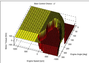
-1000 -500 0 500 1000 0 50 100 150 200 250 300 350 -100 0 100
Engine Angle [deg] Best Control Choice - u*
Engine Speed [rpm]
Figure 5 - IMEC control table
The DMEC was realized by wrapping a copy of the plant model with an API similar to the one used for the CDA. A DOE was used to search feasi-ble actions. The resulting code structure is identical to Figure 2. The optimal action was chosen to mini-mize (9).
For both of these controllers, the problem of starting the engine from any initial condition was solved. The solution involved the counter-intuitive approach of spinning the engine backwards, then reversing direction to allow enough energy to be stored in the inertia to overcome the spring force. From a model and a control objective, an optimal controller with very complex behaviors was numeri-cally generated in less than 10 minutes on a single PC (3GHz, 2Gb RAM). Furthermore, a similar problem with four states was solved in less than three hours. Of course the power of this approach can only be realized once a sufficient level of tool support is available so that the time required to set up the analysis is on the same order as the solution time.
3.1 Direct vs Indirect MEC
Ideally, both an IMEC and DMEC will re-sult in identical behaviors. However, differences in approximation schemes and interpolation can results in appreciable differences. In many cases, while In-direct MEC is simpler to realize in a model, there are good reasons to implement a controller with the complexity and computational cost of a Direct MEC. As an example, consider the previous prob-lem. The value function, V(x), was found using the
Control Design Algorithm (CDA). The IMEC con-troller was designed by solving for the best electric machine torque for a set of engine angles and speeds on a regular grid. For engine states which occur off this grid, multi-linear interpolation was used to cal-culate the control action. When the IMEC was used in an engine start simulation, if the optimal torque transitioned between positive and negative, the inter-polation caused a smooth change in the torque be-cause of the continuity imposed by interpolation.
Alternatively, consider a Direct MEC. Be-cause of the characteristics of the dynamic pro-gramming equations and the value function, the op-timal choices are either full positive or full negative torque. This results in an instantaneous, non-continuous change in torque. When plotted as in Figure 6, the difference between the control inputs and the state evolution of the system can be seen. The interpolation due to the approximation in the IMEC results in artifacts in the control actions and a slight loss of performance in the system. Mathe-matically this means that more detail is required to resolve
u
*x
, the function that we are ultimatelytrying to formulate, than to resolve
V
x
.There are cases where an IMEC is superior to a DMEC approach (e.g. [26] illustrates just such a case). In general, an IMEC implementation is supe-rior when both the action set is continuous and the optimal actions are continuous. The DMEC approach is superior when either the action set is discrete or the optimal actions are not continuous with respect to the state. One example where DMEC is clearly superior is where the motor is controlled by selecting the state of a switch inverter. In this case, the action set consists of a finite set of choices for switch con-figuration and the optimal actions are not continuous with respect to the state.
4 Implementation of optimization
al-gorithms
One of the challenges in Direct Model Em-bedded Control is the implementation of an opti-mizer. While this work was performed using a De-sign of Experiments (DOE) to select optimal actions, this approach becomes intractable when equality constraints and larger dimensional actions sets are considered. Towards the goal of supporting these classes of problems, a gradient-based optimizer was developed. One of the goals in developing this opti-mizer was to fully implement the optiopti-mizer in Mode-lica. By fully implementing in Modelica, all of the information used by the optimizer would be accessi-ble for speed improvements by the compiler. Should native support for model embedding become avail-able, all equations associated with a Direct MEC would be accessible to the compiler for speed im-provement. Additionally, since the embedded simu-lations in a DMEC can be completely decoupled from each other, simulation tools could easily exploit the coarse grained parallelism on multi-core CPUs by running several embedded simulations concur-rently when conducting searches in the optimizer (e.g. line searches and numerical gradients).
The optimizer was developed in Modelica to solve a constrained optimization problem which is generally stated in negative null form [30] as
min
. .
0
0
objective inequalities equalitiesf
s t
g
h
.
(26)
To implement a gradient optimizer, the optimizer functionality was separated from the objective func-tion (
f
objective), the inequality constraint functions (g
inequalities), and the equality constraint functions (h
equalities). The optimizer was designed under the assumption that the inequality constraint functions are all in negative null form: feasible inequality con-straints are less than or equal to zero. The objective function was assumed to be a minimization objec-tive. Since Modelica does not (yet) support the con-cept of methods or passing of functions as argu-ments, the optimizer was designed to use static in-heritance. For this reason, the objective and con-straint functions are replaceable functions within an optimizer package.One feature of this library, that is not com-monly available, is the ability to handle functions
which are undefined over some region. The domain of the objective and constraints may not be known a priori. This occurs with MEC applications because the objective (e.g. equation (9)) and constraint func-tions (e.g. equation (11)) are typically evaluated us-ing a solver. The solver may not find a solution. Hence, classical algorithms must be modified to re-cover from undefined evaluations.
Implementation of this capability was prob-lematic because of the lack of numeric support for a real value which represents the concept of an unde-fined quantity. Either a native capability similar to Matlab’s ® ‘NaN’, or operator overloading with the ability to extend a class from real numbers would have simplified implementation.
In this library, Modelica.Constants.inf was used to indicate that a function call was undefined. However, the language specification does not define behavior for operations (e.g. addition, subtraction, multiplication, division) on Modelica.Constants.inf. Therefore, all functions and statements which oper-ated on variables that might be assigned a value of Modelica.Constants.inf required conditional expres-sions to ensure expected behavior.
While this optimization library will not be publicly released, it is available for further develop-ment. Contact the lead author for a copy.
5 Recommendations
While it is possible to realize both IMEC and DMEC controllers using Modelica 2.2, the addi-tion of a standard optimizaaddi-tion library and native support for embedded model simulation would vastly simplify implementation and maintenance.
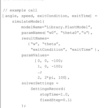
Towards the goal of simplifying implemen-tation of MEC, a recommended language improve-ment is the addition of a ‘model simulate’ function. The function would accept arguments that specify the model to simulate, the parameter values to use in each simulation, the outputs to return, and any solver specific settings. The solver should be able to be configured to solve both initialization problems and simulation problems. For efficiency in evaluation, the function should support both a scalar and vector lists of parameters. In addition to results which are associated with the model, there should be results associated with the solver. These results should be sufficient to diagnose solver failures. At a mini-mum, these should include the final time in the evaluation and an indication of whether the simula-tion successfully completed. A sample funcsimula-tion
defi-nition along with an example invocation are shown in Figure 7.
function simulateModel
input String modelName;
input String paramNames[:];
input String resultNames[:];
input Real
paramValues[:,size(paramNames,1)];
input SettingsRecord solverSettings;
output Real results[size(paramValues,1), size(resultNames,1)]; … end simulateModel; // example call
[angle, speed, exitCondition, exitTime] = simulateModel( modelName=“Library.PlantModel”, paramNames{“w0”, “theta0”,”u”}, resultNames= {“w”, “theta”, “exitCondition”, “exitTime” }, paramValues= [0, 0, -100; 1, 0, -100; …; 2, 2*pi, 100], solverSettings = SettingsRecord( stopTime=1.0, fixedStep=0.1) );
Figure 7 - Model evaluation
It is important to point out that the goal is to be able to invoke such a function from within a run-ning model and not simply as a command line analy-sis option. As previously mentioned, the ability to directly express such nested simulation relationships makes posing MEC problems much easier. If the MEC problem could also directly express the “opti-mization problem” associated with MEC then tools could also bring the underlying symbolic informa-tion to bear on efficient gradient evaluainforma-tion as well.
One remaining issue for DMEC problems is the initialization of state variables in the embedded model. For DMEC problems we typically want the embedded model to start at the current state of the parent simulation. Said another way, the current val-ues of the states in the parent simulation should be
used as initial conditions in the nested simulation. Of course, it is possible using the function in Figure 7 to establish such a mapping but hopefully the lan-guage design group will consider alternatives that would be less tedious and error prone.
6 Conclusions
It is tractable to numerically synthesize near optimal (or approximately minimal) controllers for many systems. While in most cases the state feed-back required for the controllers may make them impractical to deploy, they can certainly be used as prototype controllers that establish performance lim-its for a given design as well as provide insights into control laws for production controllers. Further-more, this approach can easily integrate into a com-bined plant-controller optimization process. This can be done by making the optimal controller a function of the plant parameters. These optimal controllers can be realized as lookup tables (IMEC) or through the use of optimization and embedded models (DMEC). An algorithmic approach to controls syn-thesis was presented. For this paper, the IMEC and DMEC approaches were applied to an engine start-ing problem to generate an optimal controller in an automated fashion.
As this work has shown, Modelica is a promising technology for rapid prototyping of sub-system designs and prototype controllers. However, lack of support for ‘model embedding’ makes devel-opment and long term maintenance problematic be-cause considerable work must be done to implement this embedding. Lacking any language standard, this work will always be tool specific. Furthermore, im-plementation of controllers which rely on optimiza-tion suffer from the lack of a standard optimizaoptimiza-tion library. While an optimization library was developed for this work, it isn’t practical for most users to make such an investment. By adding both language sup-port to express the essential aspects of model em-bedding and optimization discussed in this paper, Modelica can evolve into a powerful technology for system development and optimization.
References
[1] H. K. Fathy,"Combined Plant and Control Optimation: Theory, Strategies, and Appli-cations," Mechanical Engineering, Univer-sity of Michigan, Ann Arbor, 2003.
[2] H. K. Fathy, P. Y. Papalambros, A. G. Ul-soy, and D. Hrovat, "Nested Plant/Controller Optimization with Application to Combined Passive/Active Automotive Suspensions." [3] H. K. Fathy, J. A. Reyer, P. Y. Papalambros,
and A. G. Ulsoy, "On the Coupling between the Plant and Controller Optimization Prob-lems," in American Control Conference, Ar-lington, Va, 2001.
[4] P. R. Kumar and P. Variaya, Stochastic Sys-tems: Estimation, Identification and Adap-tion. Englewood Cliffs, New Jersey: Prentice Hall, 1986.
[5] D. Bertsekas, Dynamic Programming and Optimal Control: Vol 2. Belmont, Mass: Athena Scientific, 1995.
[6] D. P. Bertsekas, Dynamic Programming and Optimal Control: Vol 1. Belmont, Mass: Athena Scientific, 1995.
[7] D. P. Bertsekas and J. N. Tsitsiklis, Neuro-Dynamic Programming. Belmont, Mass: Athena Scientific, 1996.
[8] M. A. Trick and S. E. Zin, "A Linear Pro-gramming Approach to Solving Stochastic Dynamic Programs," Carnegie Mellon Uni-versity 1993.
[9] M. A. Trick and S. E. Zin, "Spline Ap-proximations to Value Functions: A Linear Programming Approach," Macroeconomic Dynamics,pp. 255-277, 1997.
[10] D. P. de Farias and B. Van Roy, "The Linear Programming Approach to Approximate Dynamic Programming," Operations Re-search, vol. 51, pp. 850-865, November-December 2003.
[11] V. F. Farias and B. Van Roy, "Tetris: Ex-periments with the LP Approach to Ap-proximate DP," 2004.
[12] D. P. de Farias,"The Linear Programming Approach to Approximate Dynamic Pro-gramming: Theory and Application," Ph.D. Dissertation, Department of Management Science and Engineering, Stanford Univer-sity, Palo Alto, Ca, 2002.
[13] D. Dolgov and K. Laberteaux, "Efficient Linear Approximations to Stochastic Ve-hicular Collision-Avoidance Problems," in Proceedings of the Second International Conference on Informatics in Control, Automation, and Robotics (ICINCO-05), 2005.
[14] G. J. Gordon, "Stable Function Approxima-tion in Dynamic Programming," January 1995.
[15] R. S. Sutton and A. G. Barto, Reinforcement Learning: An Introduction. Cambridge, Mass: MIT Press, 1999.
[16] R. Munos and A. Moore, "Barycentric Inter-polators for Continuous Space and Time Re-inforcement Learning," Advances in Neural Information Processing Systems, vol. 11, pp. 1024-1030, 1998.
[17] R. Munos and A. Moore, "Variable Resolu-tion DiscretizaResolu-tion in Optimal Control," Ma-chine Learning, vol. 1, pp. 1-24, 1999. [18] J. M. Lee and J. H. Lee, "Approximate
Dy-namic Programming Strategies and Their Applicability for Process Control: A Review and Future Directions," International Jour-nal of Control, Automation, and Systems, vol. 2, pp. 263-278, September 2004.
[19] D. P. de Farias and B. Van Roy, "Approxi-mate Value Iteration with Randomized Poli-cies," in 39th IEEE Conference on Decision and Control Sudney, Australia, 2000.
[20] D. P. de Farias and B. Van Roy, "Approxi-mate Value Iteration and Temporal-Difference Learning," in IEEE 2000 Adap-tive Systems for Signal Processing, Commu-nications and Control Symposium, 2000, pp. 48-51.
[21] B. Van Roy and J. N. Tsitsiklis, "Stable Lin-ear Approximations to Dynamic Program-ming for Stochastic Control Problems with Local Transitions," Advances in Neural In-formation Processing Systems, vol. 8, 1996. [22] P. W. Keller, S. Mannor, and D. Precup,
"Automatic Basis Function Construction for Approximate Dynamic Programming and Reinforcement Learning."
[23] V. C. P. Chen, D. Ruppert, and C. A. Shoe-maker, "Applying Experimental Design and Regression Splines to High Dimensional Continuous State Stochastic Dynamic Pro-gramming," Operations Research, vol. 47, pp. 38-53, January-February 1999.
[24] C.-C. Lin, H. Peng, and J. W. Grizzle, "A Stochastic Control Strategy for Hybrid Elec-tric Vehicles," in Proceedings of the 2004 American Control Conference, 2004, pp. 4710-4715 vol. 5.
[25] E. D. Tate,"Techniques of Hybrid Electic Vehicle Controller Synthesis," Electrical Engineering: Systems, University of Michi-gan, Ann Arbor, MichiMichi-gan, 2007.
[26] E. Tate, J. Grizzle, and H. Peng, "Shortest Path Stochastic Control for Hybrid Electric Vehicles,"Internation Journal of Robust and Nonlinear Control, 2006.
[27] I. Kolmanovsky, I. Siverguina, and B. Ly-goe, "Optimization of Powertrain Operating Policy for Feasibility Assessment and Cali-bration: Stochastic Dynamic Programming Approach," in Proceedings of the American Control Conference, Anchorage, AK, 2002, pp. 1425-1430.
[28] J.-M. Kang, I. Kolmanovsky, and J. W. Grizzle, "Approximate Dynamic Program-ming Solutions for Lean Burn Engine After-treatment," in Proceedings of the 38th Con-ference on Decision & Control, Phoenix, Arizona, 1999, pp. 1703-1708.
[29] C.-C. Lin, H. Peng, J. W. Grizzle, and J.-M. Kang, "Power Management Strategy for a Parallel Hybrid Electric Truck," IEEE Transactions on Control Systems Technol-ogy,vol. 11, pp. 839-849, November 2003. [30] P. Y. Papalambros and D. J. Wilde,
Princi-ples of Optimal Design: Models and Compu-tation, 2 ed. New York, New York: Cam-bridge University Press, 2000.
[31] J. Rust, "Using Randomization to Break the Curse of Dimensionality," 1996.
[32] S. Boyd and L. Vendenberghe, Convex Op-timization. New York, N.Y.: Cambridge University Press, 2004.
[33] P. E. Gill, W. Murray, and M. H. Wright, Practical Optimization. New York, N.Y.: Academic Press, 1981.
[34] D. R. Jones, C. D. Peritunen, and B. E. Stuckman, "Lipschitzian Optimization with-out the Lipschitz Constant," Journal of Op-timization Theory and Applications, vol. 79, pp. 157-181, 1993.
[35] A. J. Booker, J. Dennis, J. E. , P. D. Frank, D. B. Serafini, V. Torczon, and M. W. Tros-set, "A Rigorous Framework for Optimiza-tion of Expensive FuncOptimiza-tions by Surrogates." [36] M. J. Sasena,"Flexibility and Efficiency En-hancements for Constrained Global Design Optimization with Kriging Approximations," Mechanical Engineering, University of Michigan, Ann Arbor, 2002.