A Framework for Speech Recognition
using Logistic Regression
Øystein Birkenes
A Dissertation Submitted in Partial Fulfillment of the Requirements for the Degree of
DOCTOR OF PHILOSOPHY
Department of Electronics and Telecommunications Norwegian University of Science and Technology
Abstract
Although discriminative approaches like the support vector machine or lo-gistic regression have had great success in many pattern recognition appli-cation, they have only achieved limited success in speech recognition. Two of the difficulties often encountered include 1) speech signals typically have variable lengths, and 2) speech recognition is a sequence labeling problem, where each spoken utterance corresponds to a sequence of words or phones. In this thesis, we present a framework for automatic speech recogni-tion using logistic regression. We solve the difficulty of variable length speech signals by including a mapping in the logistic regression framework that transforms each speech signal into a fixed-dimensional vector. The mapping is defined either explicitly with a set of hidden Markov models (HMMs) for the use in penalized logistic regression (PLR), or implicitly through a sequence kernel to be used with kernel logistic regression (KLR). Unlike previous work that has used HMMs in combination with a discrim-inative classification approach, we jointly optimize the logistic regression parameters and the HMM parameters using a penalized likelihood crite-rion. Experiments show that joint optimization improves the recognition accuracy significantly. The sequence kernel we present is motivated by the dynamic time warping (DTW) distance between two feature vector se-quences. Instead of considering only the optimal alignment path, we sum up the contributions from all alignment paths. Preliminary experiments with the sequence kernel show promising results.
A two-step approach is used for handling the sequence labeling prob-lem. In the first step, a set of HMMs is used to generate an N-best list of sentence hypotheses for a spoken utterance. In the second step, these sentence hypotheses are rescored using logistic regression on the segments in the N-best list. A garbage class is introduced in the logistic regression framework in order to get reliable probability estimates for the segments in the N-best lists. We present results on both a connected digit recognition task and a continuous phone recognition task.
Preface
This dissertation is submitted in partial fulfillment of the requirements for the degree ofPhilosophiae Doctor (PhD) at the Norwegian University
of Science and Technology (NTNU). My main supervisor has been Asso-ciate Professor Magne Hallstein Johnsen at the Department of Electron-ics and Telecommunications, NTNU. My co-supervisor has been Dr. Tor Andr´e Myrvoll, who was affiliated with the Department of Electronics and Telecommunications, NTNU until January 2007. He is now with SINTEF, Trondheim.
The work was carried out in the period from January 2003 to April 2007. In addition to the research activity, the work included the equivalent of one year of full-time course studies, as well as one year of teaching assistant duties. I spent most of my time with the Signal Processing Group at the Department of Electronics and Telecommunications, NTNU, but I also had the chance to do research abroad twice. In the period from March to December 2005 I visited The Institute of Statistical Mathematics (ISM), Tokyo, Japan, under the supervision of Associate Professor Tomoko Matsui. I went there again the following year, from June to August 2006.
The work was funded by a scholarship from the Research Council of Norway through the BRAGE project, which is a part of the language tech-nology programme KUNSTI. For my first stay in Japan, I was supported by the Japan Society for the Promotion of Science (JSPS) Postdoctoral Fellowship for Foreign Researchers and JSPS Grant-in-Aid for Scientific Research (B) 16300036 and (C) 16500092. For my second stay in Japan, I received a grant from the Scandinavia-Japan Sasakawa Foundation (SJSF).
Acknowledgements
First, I would like to thank my supervisor, Associate Professor Magne Hall-stein Johnsen, for his guidance and suggestions. I would also like to thank my co-supervisor, Dr. Tor Andr´e Myrvoll, for his invaluable help and for all our technical and non-technical discussions on various topics like Mac,
Japan, food, etc.
A large portion of the research leading up to this thesis was conducted while I visited the Institute of Statistical Mathematics (ISM) in Tokyo, Japan. I am indebted to Associate Professor Tomoko Matsui, for being my host at ISM in Japan, for introducing me to the exciting field of logistic regression, and for continuously motivating me. I am very grateful to Pro-fessor Kunio Tanabe for our enjoyable meetings where he taught me many things about statistics in a way that I could easily understand. I would also like to thank my office mate and friend Dr. Marco Cuturi for fruitful collaboration, and Dr. St´ephane S´en´ecal for our friendship and technical discussions.
In my last year as a PhD student, I was fortunate to meet Dr. Sabato Marco Siniscalchi, with whom I enjoyed enlightening discussions and collab-oration. He also gave me a thorough review of my thesis. Other reviewers of my thesis that I particularly would like to thank are my fellow PhD students Svein Gunnar Pettersen, Andreas Egeberg, and Trond Skogstad.
There are many people at the Signal Processing Group at NTNU that I would like to thank. In particular, I would like to thank my office mate through more than two years, Vidar Markhus. Together we discussed many ideas on how to improve speech recognition. I am also grateful to Ole Morten Strand for our numerous discussions on speech recognition. Among other people that I would like to thank are my colleagues and friends Greg Harald H˚akonsen, Fredrik Hekland, Anna Na Kim, S´ebastien de la Kethulle de Ryhove, Bojana Gaji´c, Saeeid Tahmasbi Oskuii, Gang Lin, Duc Van Duong, Dyre Meen, and Pierluigi Salvo Rossi.
Finally, I would like to thank my parents for their moral support and for always being there for me, and my dear Yoshiko for all her love and encouragement.
Oslo, July 2007 Øystein Birkenes
Contents
1 Introduction 1
1.1 Pattern Recognition and Classification . . . 2
1.2 Contributions of this Thesis . . . 4
1.2.1 Contributions to the Logistic Regression Framework 5 1.2.2 Isolated-Word Speech Recognition using Logistic Re-gression . . . 5
1.2.3 N-Best Rescoring using Logistic Regression on Seg-ments . . . 6
1.3 Related Work . . . 6
1.4 Outline . . . 8
2 Logistic Regression 9 2.1 Penalized Logistic Regression . . . 9
2.1.1 Determining the Regularization Parameterδ . . . . 17
2.1.2 Garbage Class . . . 20
2.1.3 Adaptive Regressor Parameters . . . 21
2.2 Kernel Logistic Regression . . . 23
2.2.1 The Kernel . . . 28
2.2.2 Sparse Approximations . . . 29
2.3 Summary . . . 30
3 Speech Recognition and Hidden Markov Models 31 3.1 Feature Extraction . . . 31
3.2 Hidden Markov Models . . . 33
3.2.1 Hidden Markov Models for Speech . . . 37
3.3 Isolated-Word Speech Recognition . . . 39
3.3.1 Discriminative Training of the HMM Parameters . . 40
3.4 Continuous Speech Recognition . . . 40
3.4.1 N-Best Lists and Lattices . . . 41
3.5 Summary . . . 42 vii
4 Isolated-Word Speech Recognition using Logistic
Regres-sion 43
4.1 Penalized Logistic Regression . . . 44
4.1.1 Adaptive Regressor Parameters . . . 48
4.2 Kernel Logistic Regression . . . 50
4.2.1 Vector Kernels . . . 50
4.2.2 Sequence Kernels . . . 51
4.3 Experiments . . . 56
4.3.1 A Thorough Analysis on the TI46 E-set . . . 57
4.3.2 Phone Classification on the TIMIT Database . . . . 69
4.4 Summary and Discussion . . . 72
5 N-best Rescoring using Logistic Regression on Segments 73 5.1 Relabeling and Rescoring Sentence Hypotheses . . . 74
5.2 Rescoring N-Best Lists . . . 75
5.2.1 Logistic Regression on Segments in N-best Lists . . 76
5.2.2 The Rescoring Procedure . . . 78
5.3 Experiments . . . 79
5.3.1 Connected Digit Recognition using the Aurora2 Database . . . 80
5.3.2 Continuous Phone Recognition on the TIMIT Database 83 5.4 Summary and Discussion . . . 87
6 Conclusions and Future Work 89 6.1 Future Work . . . 90
A Proofs of Lemmas 95 A.1 Proof of Lemma 2.1.1 . . . 95
A.2 Proof of Lemma 2.1.2 . . . 97
A.3 Proof of Lemma 2.1.4 . . . 98
A.4 Proof of Lemma 2.2.1 . . . 100
A.5 Proof of Lemma 2.2.2 . . . 101
A.6 Proof of Lemma 4.1.1 . . . 102
A.7 Proof of Lemma 4.1.2 . . . 103 B Estimation of Hidden Markov Model Parameters 105
Notation and Symbols
x Scalars are typeset in non-bold lowercase x Vectors are typeset in bold lowercaseX Vector sequences and matrices are typeset in bold upper-case (in Chapters 1 and 2,X is more general and is taken to mean an object of any type)
WT The transpose of W
|W| The determinant of W
kWk The Euclidean norm of W
traceW The trace of square matrix W, which is the sum of the diagonal elements
vecW orW~ The columns of matrixW stacked into a vector diagw A diagonal matrix containing the elements of vector w
∇W The gradient matrix of partial derivatives wrt.W
∇2
W The Hessian matrix of second partial derivatives wrt. W
⊗ The Kronecker product
∝ Proportional to
R The set of real numbers N The set of natural numbers
Chapter 1
Introduction
Automatic speech recognition is the task of automatically converting speech
into text. It has applications in many areas, including dictation, com-mand and control, and automatic telephone services, just to name a few. The problem is far from trivial, a statement that is supported by the vast amount of research publications within the area of speech recognition over the last few decades.
The most popular approach to speech recognition is thehidden Markov model (HMM) framework [Rabiner, 1989]. Although the HMM framework
has a range of attractive features for speech recognition, it also has some shortcomings that limit the achievable recognition performance. First, the HMM makes some incorrect assumptions about the speech signal and is therefore not the true model for speech. Second, the HMM parameters are typically estimated using the maximum likelihood (ML) criterion. This means that the parameters for each class are estimated independently of the other classes so as to best describe the generation of the observations. This is different from minimizing the probability of recognition error, which is the ultimate goal of speech recognition, and ML is therefore suboptimal. Moreover, there is no straightforward way of obtaining a confidence measure for the recognition decision.
Penalized logistic regression(PLR) [Hoerl and Kennard, 1970; Anderson
and Blair, 1982] and kernel logistic regression (KLR) [Green and Yandell,
1985; Jaakkola and Haussler, 1999b], collectively referred to as logistic re-gression, are statistically well-founded classification approaches. Although
the methods have been around for a while, they have not been particularly popular for pattern recognition applications lately, partly due to the success of thesupport vector machine (SVM) [Vapnik, 1995; Sch¨olkopf and Smola,
2002]. Recent work [Jaakkola and Haussler, 1999b; Zhu and Hastie, 2001, 2005] has shown that logistic regression has many similar theoretical
erties as SVM, and it is comparable to SVM when it comes to classification accuracy. Unlike SVM, however, logistic regression outputs the conditional probability of a class given an observation, and has a natural generalization to the multi-class case. These additional features are important in many practical pattern recognition problems, including speech recognition.
If we attempt to design a speech recognizer with logistic regression (or SVM), we face two major difficulties. First, speech signals typically have
variable lengths, even repeating utterances of the same word from the same
speaker, while logistic regression is a static classifier, meaning that the ob-servations are assumed to be fixed-dimensional vectors. Second, a speech signal corresponds to a sequence of words, and each word corresponds to an unknown portion of the speech signal. Thus, speech recognition is a
sequence labeling problem, with unknown segmentation, while logistic
re-gression is designed to predict a single label only.
In this thesis we present a framework for automatic speech recogni-tion using logistic regression. We solve the problem with variable-length speech signals by including a mapping in the logistic regression framework. The mapping maps a variable-length speech signal into a fixed-dimensional vector and is defined either explicitly with the use of a set of HMMs, or implicitly through a kernel function. A two-step approach is chosen for handling the sequence labeling problem. In the first step, a set of HMMs is used to generate an N-best list of sentence hypotheses for a spoken ut-terance. In the second step, these sentence hypotheses are rescored using logistic regression on the segments in the N-best list. A series of experi-ments demonstrate the power and show the potential of the framework.
We start this introductory chapter by giving a short review of pattern recognition and classification. Then, in Section 1.2 we list the major con-tributions of this thesis, and in Section 1.3 we compare the concon-tributions with related work. Finally, in Section 1.4 we give an overview of the outline of the rest of the thesis.
1.1
Pattern Recognition and Classification
Automatic speech recognition is essentially apattern recognition problem,
where the goal is to recognize patterns in speech as words. In general, pattern recognition involves preprocessing, feature extraction and classi-fication [Devroye et al., 1996; Duda et al., 2001]. In this thesis, we will rely on existing preprocessing and feature extraction methods for speech recognition, and focus our attention only on the classification step.
In statistical classification, we assume that (X, y)∈ X × Y is a random pair drawn according to a probability distribution p(X, y). We consider
1.1 Pattern Recognition and Classification 3
X ∈ X to be a suitable representation of an observable pattern, and y ∈
{1, . . . , C} to be an unobservable label describing which class the pattern
belongs to. For example, X can be a sequence of Mel-frequency cepstral coefficients (MFCC) andy can represent the word label ofX. The goal in classification is to construct a decision rule h from the input space X to the set of class labelsY which is optimal in some sense. Mathematically, a decision rule can be written as
h:X → Y (1.1)
X 7→y,ˆ (1.2)
where ˆy=h(X) for any X ∈ X. Usually we are interested in the decision rule which gives the least probability of misclassification.
If the true distribution p(X, y) were known, the optimal decision rule would be theBayes decision rule [Berger, 1985], which is
ˆ
y= arg max
y∈Y p(y|X) (1.3)
= arg max
y∈Y p(X|y)p(y). (1.4)
In the second equality above, we have used Bayes rule and omitted the denominator p(X) since it is independent of y and does not contribute to the decision.
In practical problems we do not know the true distribution p(X, y), so other decision rules are called for. In this thesis we will focus on the construction of a decision rule by the use of a finite set D =
{(X(1), y(1)), . . . ,(X(N), y(N))} of samples assumed to be drawn indepen-dently according to p(X, y). These samples are called the training data
and the approach taken to infer a decision rule from training data is known assupervised learning.
Within the framework of supervised learning there are two main ap-proaches. The first approach, known as the generative approach, aims at
modeling the jointgenerative model p(X, y) of observationsX and classes y. This is usually done through modeling of the class-conditional distri-butions p(X|y) and the class prior p(y). The estimated distributions are substituted for the true distributions in (1.4). Conventional speech recog-nition is done using this approach, where each observationX is a sequence of feature vectors extracted from a speech signal. The class-conditional distributionsp(X|y) are then typically obtained from HMMs.
The other main approach to supervised learning is called the discrim-inative approach. In this approach, the conditional distributionp(y|X) of class labels given an observation is modeled and substituted for the true one
in (1.3). Logistic regression is an example of this approach. Other discrimi-native approaches include kernel methods such as SVM, which approximate the decision rule in (1.3) in a discriminative way without explicitly provid-ing the conditional probabilities p(y|X).
Both the generative approach and the discriminative approach to learn-ing classifiers have their strengths and weaknesses [Ng and Jordan, 2002; Ulusoy and Bishop, 2005]. The generative approach can handle missing or partially labeled data, and can make use of a combination of small amounts of expensive labeled training data with large quantities of cheap unlabeled training data. Moreover, generative models can readily handle compo-sitionality, which in speech recognition terms means that long linguistic units such as words can be modeled by concatenating a set of models for short linguistic units such as phones. On the other hand, in the discrim-inative approach the decision rule is learnt in a more direct way than in the generative approach, without making assumptions on the distribution of the observations. Modeling effort is spent in the confusable regions of the observation space that are important for classification, whereas in the generative approach an attempt is made to accurately model regions in the observation space that may be irrelevant for the outcome of the resulting decision rule.
Since the generative approach and the discriminative approach have complementary strengths and weaknesses, it seems natural to attempt to combine them. Discriminative training is one such approach, where a
gen-erative model is trained using a discriminative criterion function. Examples of discriminative training approaches that have been successfully applied to speech recognition include maximum mutual information (MMI) [Bahl
et al., 1986] and minimum classification error (MCE) [Juang et al., 1997].
Another combination approach is to use a discriminative classifier such as logistic regression or SVM that incorporates a generative model [Jaakkola and Haussler, 1999a; Smith and Gales, 2002]. The latter is the approach taken in this thesis.
1.2
Contributions of this Thesis
This thesis provides a study of logistic regression and its use in automatic speech recognition. Both penalized logistic regression (PLR) and kernel logistic regression (KLR) are considered. Contributions are made in the logistic regression framework, as well as in the application to isolated-word speech recognition and N-best rescoring for continuous speech recognition. Parts of the work has been published in [Birkenes et al., 2005, 2006a,b, 2007; Cuturi et al., 2007].
1.2 Contributions of this Thesis 5
1.2.1 Contributions to the Logistic Regression Framework
While most presentations of logistic regression in the literature assume the observations to be fixed-dimensional vectors (e.g., [Jaakkola and Haussler, 1999b; Tanabe, 2001a,b; Zhu and Hastie, 2001, 2005]), we present a more general logistic regression framework that allows observations to be objects of arbitrary type. The generalization is trivial, however, since we simply redefine a nonlinear mapping such that it maps an observation of any par-ticular type into a fixed-dimensional vector. The motivation for this simple generalization is that we would like to use logistic regression for speech recognition, where each observation is a sequence of feature vectors or a
time series.
In this thesis, we also provide necessary proofs of derivatives in the logistic regression framework, many of which are missing in the literature. In addition, we provide derivations of the formulas for the determination of the regularization parameter in PLR with the use of a Bayesian information criterion (ABIC) [Akaike, 1980].
The two major contributions to the logistic regression framework, how-ever, are 1) adaptive regressor parameters, which allows for more flexible
decision boundaries for PLR, and 2) agarbage class, to ensure proper
be-haviour for the prediction of atypical observations for both PLR and KLR.
1.2.2 Isolated-Word Speech Recognition using Logistic Re-gression
The major difficulty in applying logistic regression to isolated-word speech recognition is that speech signals typically have variable lengths. We present solutions to this problem in the form of several mappings from variable-length time series into fixed-dimensional vectors. The mappings are either defined explicitly, as in PLR, or implicitly through a kernel to be used with KLR. The mappings for PLR are based on a set of HMMs. They include a mapping of a time series into a vector of the likelihoods of each HMM, and a mapping into a vector of likelihood-ratios of each model and its corresponding anti-model. With the use of adaptive regressor param-eters, which in this case are the HMM paramparam-eters, we obtain a powerful discriminative classifier for speech signals that combines the advantages of the generative learning approach and the discriminative learning approach. We present two families of kernels to be used with KLR. The first family consists of vector kernels (e.g., Gaussian or polynomial) that operate on pairs of time series via the fixed-dimensional vectors obtained from either of the explicit mappings. The second family are sequence kernels that operate directly on pairs of time series. A particular member of this family
is theglobal alignment (GA) kernel [Cuturi et al., 2007], which we recently
proposed. With the latter family of kernels, KLR is a purely discriminative approach for isolated-word speech recognition.
Experiments on the E-set of the TI46 database compare the various approaches. Also, a phone classification experiment on the TIMIT database [Lamel et al., 1986] using PLR with adaptive regressor parameters is done.
1.2.3 N-Best Rescoring using Logistic Regression on Seg-ments
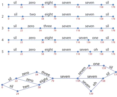
We choose a two-step approach to continuous speech recognition. In the first step, a set of HMMs is used to generate an N-best list of sentence hypotheses for a spoken utterance. In the second step, these sentence hy-potheses are rescored using logistic regression on the segments in the N-best list. The new sentence scores are either used directly to reorder the sen-tence hypotheses in the N-best list, or they are interpolated with the HMM likelihoods of the corresponding sentence hypotheses before reordering. We argue that logistic regression with a garbage class is necessary in this ap-proach.
The N-best rescoring approach is tested on the Aurora2 database [Pearce and Hirsch, 2000] for connected digit recognition. We also per-form continuous phone recognition using the TIMIT database [Lamel et al., 1986].
1.3
Related Work
In this section, we mention various papers that are related to the work presented in this thesis. We start with papers that use a set of HMMs as a preprocessor for logistic regression or SVM in order to perform isolated-word speech recognition. Then we cite two papers that use sequence kernels that operate directly on pairs of time series. Finally, we mention a paper that resembles the way we do continuous speech recognition.
Perhaps the first paper to use HMMs in order to map time series into fixed-dimensional vectors for the use in logistic regression and SVM was [Jaakkola and Haussler, 1999a]. Their presentation was general, however, in the sense that they targeted a range of pattern recognition applications, and not only speech recognition with HMMs. They proposed the Fisher score mapping, which maps a time series into the gradient space of a single HMM.
Furthermore, they constructed a kernel from the Fisher score mapping, known as theFisher kernel. The kernel was used in binary SVM and
1.3 Related Work 7
were trained separately with the use of two different criteria. This is also the case for the other methods presented in this section.
In [Smith and Gales, 2002], the authors considered the use of the Fisher score in speech recognition. They used binary SVM and considered the use of two HMMs instead of only one HMM as in [Jaakkola and Haus-sler, 1999a]. Moreover, they proposed to append the Fisher score with the likelihood, likelihood-ratio, or even higher order derivatives of the HMM parameters.
In [Layton and Gales, 2006] the authors built on the work in [Smith and Gales, 2002] and introduced theconditional augmented (C-Aug) model. The
C-Aug model resembles to a high degree the multinomial logistic regression model presented in this thesis. A set of one HMM for each class is used in the mapping, but unlike our approach, where the model for each class probability depends on all HMMs, the C-Aug model for a class probability depends only on the HMM for that particular class. Moreover, training of the C-Aug model is done using the maximum likelihood criterion without a penalty term.
In [Abou-Moustafa et al., 2004], the authors presented a class-independent mapping that makes use of the HMMs of all the classes. In their approach, each element of the mapped observation is the log-likelihood of a HMM. The authors used SVM as the discriminative classifier, and pre-sented results on a handwriting recognition task.
For the purely discriminative approach of using a sequence kernel for speech recognition, there is not much to find in the literature. Notable papers include [Shimodaira et al., 2002] and [Bahlmann et al., 2002]. The former paper introduced the dynamic time alignment kernel (DTAK) for
applications in speech recognition, while the latter paper introduced a ker-nel for the use in handwriting recognition. In both papers, they introduced a sequence kernel directly operating on pairs of time series. The kernels are motivated by the dynamic time warping (DTW) [Rabiner and Juang,
1993] algorithm. Both kernels are defined as the alignment score along the optimal alignment path, and they are not positive definite in general. In this thesis we present theglobal alignment (GA) kernel [Cuturi et al., 2007].
The GA kernel sums up the contributions for all the alignment paths, and it can be shown to be positive definite under mild conditions.
In [Ganapathiraju et al., 2004], the authors presented a hybrid HMM/SVM approach for continuous speech recognition using the N-best rescoring paradigm. Their method addressed both the issue of variable-length sequences and the issue of sequence labeling with unknown seg-mentation, but it had several weaknesses. Since the problem of segments (phones) with varying lengths was solved by discarding all but a fixed num-ber of feature vectors, much information in the speech signals was lost.
Moreover, in the rescoring of the N-best lists, sentences with deletion and insertion errors could not be corrected. In this thesis we introduce the con-cept of a garbage class in order to rescore all hypotheses in an N-best lists,
which implies that substitution errors, insertion errors and deletion errors may be corrected.
1.4
Outline
The outline of the thesis is as follows. In Chapter 2 we present logistic regression, including PLR and KLR. Chapter 3 is a review of HMMs and the conventional way of doing automatic speech recognition. In Chapter 4 we consider the application of logistic regression to isolated-word speech recognition. Chapter 5 is devoted to the application of logistic regression to N-best rescoring. Finally, Chapter 6 contains the conclusions and a section about future work.
Chapter 2
Logistic Regression
We use the termlogistic regressionto refer to bothpenalized logistic regres-sion (PLR) and its dual formulation which is calleddual penalized logistic regression (dPLR), or more commonly kernel logistic regression (KLR).
Many authors have presented the framework of logistic regression in the context of multiclass classification [Jaakkola and Haussler, 1999b; Tanabe, 2001a,b; Zhu and Hastie, 2001, 2005]. The various authors use different approaches to explain the theory. In this chapter we present the theory of both PLR and KLR using mostly the approach taken in [Tanabe, 2001a,b]. Our presentation is somewhat more general, however, in that we allow the inputs to be of arbitrary form, and not only fixed-dimensional vectors which is often assumed. We do this in order to prepare for the following chapters, where the inputs are sequences of feature vectors extracted from speech signals.
We start by explaining the PLR in Section 2.1. In Section 2.1.1 we consider a method for determining the regularization parameter, and in sections 2.1.2 and 2.1.3 we introduce the concepts of a garbage class and adaptive regressor parameters, respectively. We present KLR in Section
2.2. Finally, Section 2.3 contains a short summary.
2.1
Penalized Logistic Regression
In this section we will see how penalized logistic regression (PLR) can be used to estimate the conditional probability distributionp(y|X) of a class labely∈ Y given an observationX ∈ X. Classification is accomplished by selecting the class label ˆygiving the largest conditional probability, that is,
ˆ
y= arg max
y∈Y p(y|X). (2.1)
-5 -4 -3 -2 -1 0 1 2 3 4 5 0.2 0.4 0.6 0.8 1
Figure 2.1: The logistic function.
In the following, we introduce a parametric model for p(y|X). Then we define the criterion function which we will use in order to estimate the parameters of the model, followed by an optimization algorithm specifically designed for this purpose.
Before presenting the general form of the logistic regression model that we will use in this thesis as a model forp(y|X), let us start by considering the simple case of C = 2 classes and real D-dimensional feature vectors x ∈ X = RD. A popular model for the conditional probability of class
y= 1 given xis
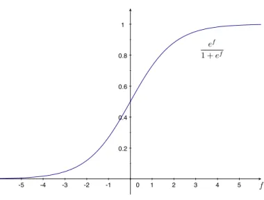
p(y= 1|x) = e f
1 +ef, (2.2)
where the discriminant function f = w1 +w2x1+· · ·+wD+1xD is a lin-ear combination (plus a bias term) of the elements of x with parameters w1, . . . , wD+1. Usually, the discriminant function is written as the inner
product f = wTx¯, where ¯x is the vector x augmented with a “1” be-fore the first element, and w is a weight vector that serves as the
pa-rameter vector of the model. Since the conditional probability of the two classes must sum to one, the conditional probability for the other class is p(y = 2|x) = 1−p(y = 1|x). The function in (2.2) is known as the lo-gistic function, or binomial logistic regressor, and, apart from being just
a squashing function that maps f into the interval [0,1], it also has good probabilistic properties in the context of classification [Jordan, 1995]. The graphic representation of the logistic function is shown in Figure 2.1.
The natural extension to classification problems with more than two classes is to model the conditional probabilities with the softmax function
2.1 Penalized Logistic Regression 11
ormultinomial logistic regressor defined by
p(y=i|x) = e fi
PC
j=1efj
fori= 1, . . . , C, (2.3) where fi = wiTx¯ is the discriminant function for class i parameterized by the weight vectorwi. Due to the probability constraintPC
i=1p(y=i|x) =
1, the weight vector for one of the classes, say wC, need not be estimated and can be set to all zeros. In this thesis however, we follow the convention in [Tanabe, 2001a] and keep the redundant representation withC non-zero weight vectors. As explained in [Tanabe, 2001a], this is done for numerical stability reasons, and in order to treat all the classes equally. We let each weight vector be a column of the matrix
W = | | w1 · · · wC | | , (2.4)
which is theparameter matrix of the model in (2.3).
With discriminant functions that are linear in the feature vectors, only linear decision boundaries between the classes in the feature spaceX =RD
can be found. A simple way to achieve nonlinear decision boundaries is to first map the features into an M+ 1-dimensional Euclidean space using a nonlinear mapping
φ:RD →RM+1 (2.5)
x7→φ(x), (2.6)
where we let the first element of the mapping be a “1” in order to accom-modate a bias term. Then, we define the nonlinear discriminant functions to be used in (2.3) as
fi=wiTφ(x;λ) fori= 1, . . . , C, (2.7) where λ is a hyperparameter vector of the mapping φ. Each element of the vectorφ(x;λ) is a function ofx. These functions are calledregressors
and they play an important role in the logistic regression framework. A straightforward generalization to the logistic regression framework can be obtained by redefining the mapping in (2.5) to
φ:X →RM+1 (2.8)
X 7→φ(X), (2.9)
whereX is the set of observations of arbitrary type. We have writtenX in the above equation in place ofxin order to emphasize that we are no longer
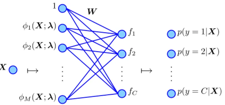
W X f1 f2 fC p(y=C|X) p(y= 2|X) p(y= 1|X)
7→
7→
1 φM(X;λ) φ2(X;λ) φ1(X;λ)Figure 2.2: The logistic regression model.
restricted to real-valued feature vectors. In fact, as long as a mapping φ can be found, X can be any nonempty set.
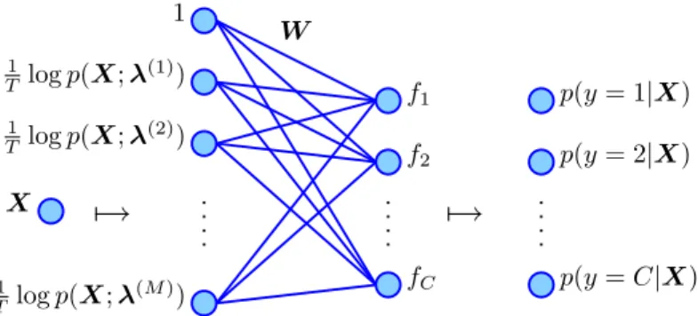
To summarize, we have introduced the following model for the condi-tional probability of classy=igivenX:
p(y=i|X,W) = e wT iφ(X;λ) PC j=1e wT jφ(X;λ) for i= 1, . . . , C, (2.10) where W is an (M + 1)×C parameter matrix with columns wi, and φ(X;λ) is a vector of M + 1 regressors with hyperparameter λ, with the first regressor being the constant “1”. We will refer to this model as the
multinomial logistic regression model, or simply as the logistic regression model. Figure 2.2 illustrates the model.
The classical way to estimate the parameter matrix W from a set of training data D={(X(1), y(1)), . . . ,(X(N), y(N))} is to maximize the like-lihood L(W;D) = N Y n=1 p(y=y(n)|X(n),W). (2.11) However, the maximum likelihood estimate does not always exist [Albert, A. and Anderson, J. A., 1984]. This happens, for example, when the mapped data set{(φ(X(1);λ), y(1)), . . . ,(φ(X(N);λ), y(N))}is linearly sep-arable. Moreover, even though the maximum likelihood estimate exists, overfitting to the training data may occur, which in turn leads to poor generalization performance. For that reason, we introduce apenalty π(W) on the parameters and find an estimate ˆW by maximizing the penalized likelihood
Pδ(W;D) =L(W;D)πδ(W), (2.12) where δ ≥ 0 is a hyperparameter used to balance the likelihood and the penalty factor. There are many ways to define the penalty factor. In this
2.1 Penalized Logistic Regression 13
thesis we follow [Tanabe, 2001a] and use a penalty of the form π(W) = C Y i=1 e−γi2wiTΣwi (2.13) =e−12 PC i=1γiwTiΣwi (2.14) =e−12traceΓW TΣW , (2.15)
whereΣis an (M+ 1)×(M+ 1) positive definite matrix, andΓis aC×C diagonal matrix with elements γ1, . . . , γC, that is,
Γ= γ1 0 ... 0 γC . (2.16)
In [Tanabe, 2001a], the author discusses various choices for the matricesΓ andΣ. One such choice that we will adopt in this thesis is explained in the following. The Γ matrix should compensate for differences in the number of training examples from each class, as well as include prior probabilities for the various classes. If we letNidenote the number of training examples from classi, andp(y=i) denote our belief in the prior probability for class i, we let the ith element ofΓ be
γi = Ni
N p(y =i). (2.17)
We let Σ be the sample moment matrix of the transformed observations φ(X(n);λ) for n= 1, . . . , N, that is,
Σ= 1 N N X n=1 φ(X(n);λ)φT(X(n);λ) (2.18) = 1 NΦΦ T, (2.19) where Φ= | | φ(1) · · · φ(N) | | (2.20)
is the (M+ 1)×N-matrix whose nth column isφ(n)=φ(X(n);λ). It is insightful to note that the above penalized likelihood parameter estimation procedure can also be interpreted in a Bayesian way, as max-imum a posteriori (MAP) estimation. This is the preferred method for
some authors (e.g., [Krishnapuram et al., 2005]). In the Bayesian formal-ism, the parameter matrix W is considered to be a random quantity, with a prior distribution p(W). If we choose p(W) ∝πδ(W), we can see from (2.13) that our choice of prior over the matrix parameter W is the prod-uct of priors over the vectors wi, where each vector wi has a multivari-ate normal distribution with zero mean and precision matrix δγiΣ. The variance-covariance matrix is the inverse of the precision matrix and is thus 1/(δγi)Σ−1. In MAP estimation, the prior p(W) is multiplied with the likelihood L(W;D) to form a quantity which is proportional to the posterior. This is the quantity which is to be maximized, and since it is the same as the penalized likelihood in (2.12), MAP estimation and maximum penalized likelihood estimation give the same result.
Maximizing the penalized likelihood in (2.12) is mathematically equiva-lent to minimizing the negative logarithm of the penalized likelihood, which can be written Plog δ (W;D) =−logPδ(W;D) (2.21) =−logL(W;D)−δlogπ(W) (2.22) =− N X n=1 logp(y=y(n)|X(n),W) +δ 2traceΓWTΣW. (2.23) In the following, we will be concerned with the minimization of the above criterion function. Let us start with two lemmas that give expressions for the gradient and the Hessian of (2.23). These expressions will be used to design an optimization algorithm in order to find an estimate of W. Lemma 2.1.1 The gradient of (2.23) is the (M+ 1)×C matrix
∇WPδlog(W;D) =Φ(P(W)T−YT) +δΣWΓ, (2.24) where P(W) = | | p(1) · · · p(N) | | (2.25)
is a C × N matrix whose nth column is a vector of the condi-tional probabilities for all classes given X(n), i.e., p(n) = [p(y(n) = 1|X(n),W), . . . , p(y(n) =C|X(n),W)]T, and Y = | | ey(1) · · · ey(N) | | (2.26)
is a C×N matrix where thenth columney(n) is a unit vector with all zeros
2.1 Penalized Logistic Regression 15
Proof See App. A
Lemma 2.1.2 The Hessian of (2.23) is
∇2 WP log δ (W;D) = N X n=1 (diagp(n)−p(n)p(n)T)⊗φ(n)φ(n)T+δΓ⊗Σ, (2.27)
where ⊗ is the Kronecker product.
Proof See App. A
It can be shown [Tanabe, 2001a] that the Hessian∇2 WP
log
δ (W;D) is a positive definite matrix. This means thatPlog
δ (W,D) is a convex function whose unique minimizer W∗ satisfies
W∗= 1 δΣ
−1Φ(YT−P(W∗)T)Γ−1. (2.28)
The above equation can be found by setting the gradient in (2.24) to zero. Note that the minimizerW∗appears on both sides of the equation, with the one on the right appearing within the nonlinear termP(W∗)T. Thus, the minimizerW∗cannot be found analytically, and we must rely on numerical methods to obtain an estimate.
We will here present an optimization algorithm for estimating the weight matrix W that makes use of both the gradient in (2.24) and the Hessian in (2.27). The algorithm was introduced in [Tanabe, 2001a] where it was called thepenalized logistic regression machine (PLRM). In this algorithm,
the weight matrix is updated iteratively using Newton’s method, where each step is
Wi+1 =Wi−αi∆Wi, (2.29) where ∆Wi is defined in
vec ∆Wi = [∇2WPδlog(Wi;D)]−1vec∇WPδlog(Wi;D). (2.30)
The factor αi is a stepsize. In order to find the update matrix ∆Wi, the inverse of the Hessian needs to be computed, and this has to be done at every step i. Computing the inverse of the Hessian is very costly, so in [Tanabe, 2001a] the author suggested to compute an approximation to ∆Wi using the conjugate gradient (CG) method [Hestenes and Stiefel, 1952; Luenberger, 1989]. This amounts to solving for ∆Wi in the equation
∇2 WP log δ (W i;D) vec ∆Wi = vec∇ WPδlog(Wi;D), (2.31)
which after substitution of (2.24) and (2.27) reduces to N X n=1 (φ(n)φ(n)T)∆Wi(diagp(n)−p(n)p(n)T) +δΣ∆WiΓ =Φ(P(WiT)−YT) +δΣWiΓ. (2.32) The CG method for solving this equation is summarized in the following algorithm, which computes an estimate of the weight matrix that minimizes the criterion function in (2.23).
Algorithm 2.1.3 (The penalized logistic regression machine [Tanabe, 2003]) Start with an initial weight matrix W0 and generate a sequence of matrices according to
Wi+1 =Wi−αi∆Wi, (2.33)
where ∆Wi is computed using the following conjugate gradient method: 1. Initialize: Start with an initial matrix∆W0i and compute the matrices
R0 and Q0: R0 =Φ(P(WiT)−YT) +δΣWiΓ − N X n=1 φ(n)φ(n)T∆W0i(diagp(n)−p(n)p(n)T)−δΣ∆W0iΓ, (2.34) Q0 = N X n=1 φ(n)φ(n)TR0(diagp(n)−p(n)p(n)T) +δΣR0Γ. (2.35)
2. Iterate: Generate a sequence (∆W1i,∆W2i, . . .) according to
αj = k PN n=1φ(n)φ(n)TRj(diagp(n)−p(n)p(n)T) +δΣRjΓk2 kPN n=1φ(n)φ(n)TQj(diagp(n)−p(n)p(n)T) +δΣQjΓk2 , (2.36) ∆Wji+1= ∆Wji+αjQj, (2.37)
2.1 Penalized Logistic Regression 17 Rj+1=Φ(P(WiT)−YT) +δΣWiΓ − N X n=1 φ(n)φ(n)T∆Wji+1(diagp(n)−p(n)p(n)T)−δΣ∆Wji+1Γ, (2.38) βj+1= k PN n=1φ(n)φ(n)TRj+1(diagp(n)−p(n)p(n)T) +δΣRj+1Γk2 kPN n=1φ(n)φ(n)TRj(diagp(n)−p(n)p(n)T) +δΣRjΓk2 , (2.39) Qj+1= N X n=1 φ(n)φ(n)TRj+1(diagp(n)−p(n)p(n)T)+δΣRj+1Γ+βj+1Qj. (2.40)
2.1.1 Determining the Regularization Parameter δ
An important issue in the penalized logistic regression framework is to de-termine the optimal value of the regularization parameterδ. This will pre-vent overfitting to the training data, thereby ensuring good generalization performance of the logistic regression model. In the following, we present two methods of how to estimate the optimal value of δ. The first method is to minimize the average cross-validation error, and the second method is to minimize a Bayesian information criterion (ABIC).
Minimization of the average cross-validation error
A relatively straightforward way to obtain an estimate of δ is through K-fold cross-validation [Duda et al., 2001]. In this method, the training set is
first partitioned intoK subsets, e.g.,K = 10. Then, training of the logistic regression model is performed on the firstK−1 parts for various values of δ. The remaining part is used for testing orvalidation. The procedure is
repeatedKtimes, such that every subset is used once for validation. In the end, the K error rates obtained for each δ are averaged, and the δ giving the lowest average error rate is chosen as the estimate.
Minimization of a Bayesian information criterion (ABIC)
An arguably more elegant way to estimate the regularization parameter δ is to minimize a Bayesian information criterion (ABIC) [Akaike, 1980;
Tanabe, 2001a]. The idea is to find the value of δ that maximizes the probability of the training data, without assuming any particular parameter matrixW. The ABIC criterion is
ABIC(δ) =−2 logp(D|δ), (2.41) wherep(D|δ) is themarginal likelihood defined by
p(D|δ) =Z p(D|W, δ)p(W|δ)dW. (2.42) Thus, we can see that minimizing the ABIC criterion is equivalent to maxi-mizing the marginal likelihood, which is the probability of the training data given δ.
The integrand in (2.42) is the posterior distribution of the model with likelihoodp(D|W, δ) =L(W;D) and priorp(W|δ). The prior distribution can be written
p(W|δ)∝δC(M+1)/2πδ(W), (2.43) whereπ(W) is the penalty factor introduced in (2.12). The normalization constants that are independent ofW andδare omitted from the right hand side above since they are irrelevant in the minimization of ABIC(δ). We now have p(D|δ)∝δC(M+1)/2 Z L(W;D)πδ(W)dW (2.44) =δC(M+1)/2 Z Pδ(W)dW (2.45) =δC(M+1)/2 Z e−Pδlog(W)dW, (2.46)
where Pδ(W) = Pδ(W;D) is the penalized likelihood in (2.12) and
Plog
δ (W) = −logPδ(W) is the negative logarithm of the penalized like-lihood. The integral in (2.46) does not have an analytic solution [Tanabe, 2001a]. An approximation to the integral is considered next.
In the following, we use the notationW~ = vecW to denote the vector-ized version of the matrixW. Furthermore, let Pe
log
δ (W) be the quadratic approximation of Plog
δ (W) about its maximizing argumentW
∗, i.e., e Plog δ (W) =P log δ (W ∗) +1 2(W~ −W~ ∗)T∇2 WP log δ (W ∗)(~ W −W~ ∗) (2.47) =Plog δ (W ∗) +q(W), (2.48)
2.1 Penalized Logistic Regression 19
whereq(W) is the quadratic form defined in (2.47). The above approxima-tion is good if Plog
δ (W) has a shape which is close to a quadratic form, in which casePe
log
δ (W)≈ P
log
δ (W). With this in mind, we write the integral in (2.46) as Z e−Pδlog(W)dW = Z e−Pδlog(W)ePelog δ (W)e−Pelog δ (W)dW (2.49) =Z ePelog δ (W)−P log δ (W)e−Pelog δ (W)dW (2.50) = Z ePe log δ (W)−P log δ (W)e−P log δ (W ∗)−q(W) dW (2.51) =e−Pδlog(W ∗)Z ePelog δ (W)−P log δ (W)e−q(W)dW (2.52) =e−Pδlog(W ∗) Z Z ePelog δ (W)−P log δ (W)f(W)dW, (2.53) where f(W) = 1 Ze −q(W) (2.54)
is a Gaussian distribution with mean W∗, covariance matrix
∇2 WP
log
δ (W
∗)−1, and normalization constant
Z = (2π)C(M+1)/2|∇2WPδlog(W∗)|−1/2, (2.55) with|·|denoting the determinant of a matrix. Now, the marginal likelihood can be written p(D|δ)∝δC(M+1)/2|∇2WPδlog(W∗)|−1/2e−Pδlog(W ∗) · Z ePe log δ (W)−P log δ (W)f(W)dW. (2.56)
Furthermore, we can write the ABIC criterion as
ABIC(δ) =−2 logp(D|δ) (2.57) ∝2Plog δ (W ∗) + log|∇2 WP log δ (W ∗)| −C(M+ 1) logδ+ correction, (2.58) where the correction term is
correction =−2 logZ ePe log
δ (W)−P
log
δ (W)f(W)dW. (2.59)
If Peδlog(W) is a good approximation to Pδlog(W), the correction term is
close to zero, and an approximate criterion can be taken to be right hand side of (2.57) without the correction term.
We can approximate the correction term by generating a set of indepen-dent samples {Wj}Jj=1 from f(W) which we substitute into the following
expression: correction≈ −2 log 1 J J X j=1 ePelog δ (Wj)−P log δ (Wj) (2.60)
The samples {Wj}Jj=1 can be generated by first generating a set of
inde-pendent samples {Uj}Jj=1 from a standard normal distribution, and then
substituting these samples into ~ Wj =W~ ∗+∇2WP log δ (W ∗)−1/2U~ j, (2.61) where∇2 WP log
δ (W∗)−1/2 is defined from the Cholesky decomposition of the covariance matrix as in ∇2 WP log δ (W ∗)−1=∇2 WP log δ (W ∗)−1/2∇2 WP log δ (W ∗)−T/2. (2.62)
To summarize, we can estimate δ by minimizing the ABIC criterion in (2.57). In practice, this is done by calculating the criterion for various values ofδ, followed by selecting the δ value giving the lowest criterion.
2.1.2 Garbage Class
In some applications, the classifier will be presented with observations X that do not correspond to any of the classes in the label set Y. As an example, consider a classifier designed for classifying handwritten digits which is presented with a letter from the English alphabet. In this situation, the classifier should return a small probability for every class inY. However, this is made impossible by the fact that the total probability should sum to 1, that is, P
y∈Yp(y|X) = 1. The solution to this problem is to introduce
a new class y =C + 1 ∈ Y0 = Y ∪ {K + 1}, called a garbage class, that
should get high conditional probability given observations that are unlikely for the classes inY, and small probability otherwise [Birkenes et al., 2007]. In order to train the parameters of the logistic regression model with such a garbage class, a set of observations labeled with a garbage label, or
garbage observations, are needed. For applications with a low-dimensional
observation setX, these garbage observations can be drawn from a uniform distribution overX. For many practical applications however,X has a very high dimensionality, so an unreasonably high number of samples must be drawn from the uniform distribution in order to achieve good performance. In such cases, prior knowledge of the nature or the generation of the possible garbage observations that the classifier will see during prediction is of great
2.1 Penalized Logistic Regression 21
value. For the example with handwritten digits, the garbage observations may be extracted from handwritten letters of the English alphabet. In Chapter 5 we will see how we can use N-best lists to generate garbage observations for continuous speech recognition.
2.1.3 Adaptive Regressor Parameters
To gain additional discriminative power it was proposed in [Birkenes et al., 2006a] to treatλas a free parameter of the logistic regression model instead of a preset fixed hyperparameter. In this setting, the criterion function can be written Plog δ (W,λ;D) =− N X n=1 logp(y=y(n)|X(n),W,λ) +δ2traceΓWTΣW, (2.63) which is the same as the criterion in (2.23), but with the dependency on λ shown explicitly. Note that also Σ depends on λ according to (2.18). The goal of parameter estimation is now to find the pair (W∗,λ∗) that minimizes the criterion in (2.63). This can be written mathematically as
(W∗,λ∗) = arg min
(W,λ)P log
δ (W,λ;D). (2.64) As already mentioned, the function in (2.63) is convex with respect to W ifλ is held fixed. It is not guaranteed, however, that it is convex with respect to λ ifW is held fixed. Therefore, the best we can hope for is to find a local minimum that gives good classification performance.
A local minimum can be obtained by using a coordinate descent ap-proach with coordinates W and λ. The algorithm is initialized with λ0.
Then the initial weight matrix can be found as W0 = arg min
W P log
δ (W,λ0;D). (2.65) The iteration step is as follows:
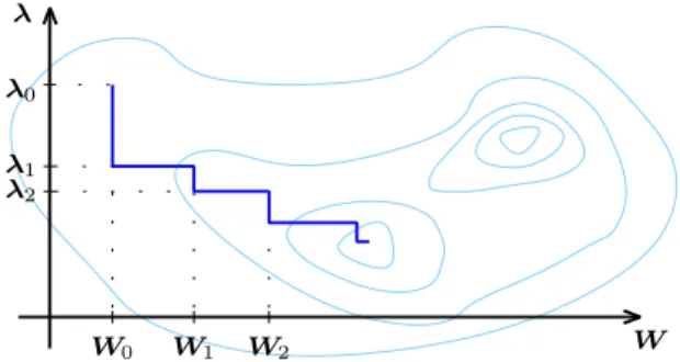
λi+1= arg min λ P log δ (Wi,λ;D), (2.66a) Wi+1= arg min W P log δ (W,λi+1;D). (2.66b) The coordinate descent method is illustrated in Figure 2.3.
For the convex minimization with respect to W, we can use the pe-nalized logistic regression machine (PLRM) in Algorithm 2.1.3. As for the
W λ W0 W1 W2 λ0 λ1 λ2
Figure 2.3: The coordinate descent method used to find the pair (W∗,λ∗) that minimizes the criterion function Plog
δ (W,λ;D).
minimization with respect to λ, there are many possibilities, two of which are the steepest descent method and the RProp method [Riedmiller and Braun, 1993]. Both these optimization methods make use of the partial derivatives of the criterion function with respect to each of the elements of theL-dimensional vectorλ. The partial derivative of the criterion function with respect toλl is given in the following lemma.
Lemma 2.1.4 The partial derivative of (2.63) with respect to the lth ele-ment of λ is ∂ ∂λlP log δ (W;λ;D) = trace δ NΦ TWΓ+PT(W)−YTWT ∂ ∂λl Φ . (2.67) Proof See App. A
When the regressor parameters are updated by minimizing the criterion function in (2.63), overfitting to the training data may occur. This typically happens when the number of free parameters in the regressor functions is large compared to the available training data. This issue is known as the curse of dimensionality. By keeping the number of free parameters in
accordance with the number of training examples, the effect of overfitting may be reduced.
Another method to reduce the effect of overfitting isearly stopping. In
this method, a part of the training set, known as avalidation set, is used to
monitor the generalization performance, i.e., the recognition accuracy on data not seen by the training algorithm, as the training algorithm iterates. Training is stopped when the generalization performance reaches a maxi-mum. Early stopping reduces the effect of overfitting by ensuring that the parameters do not deviate too much from their initial values.
2.2 Kernel Logistic Regression 23
A third way to reduce the effect of overfitting is to add a penalty term for the regressor parameters to the criterion function in (2.63). Let us assume that each elementλi of theL-dimensional vectorλhas a Gaussian prior with meanµi and variance σi2 that are known. Then, a penalty term for the whole vector can be written
π0(λ) = L Y i=1 e−2σ12(λi−µi) 2 (2.68) =e− 1 2 PL i=1σ12 i (λi−µi)2 (2.69) =e−12(λ−µ) TΣ0(λ−µ) , (2.70)
where µ is a vector of all means µi, and Σ0 is a diagonal matrix with elements 1/σ2
i. The criterion function including a penalty for the regressor parameters is then Plog δ,δ0(W,λ;D) =− N X n=1 logp(y=y(n)|X(n),W,λ) +δ2traceΓWTΣW +δ 0 2(λ−µ)TΣ0(λ−µ), (2.71) whereδ0 is a regularization parameter for the regressor parameters.
2.2
Kernel Logistic Regression
Kernel logistic regression (KLR) is a generalization of penalized logistic
regression. It allows for more flexible decision boundaries by letting the number of regressors grow to a very large number, or even infinite, without much increase in computational cost. Moreover, in KLR, we are not re-quired to make specific choices of the mappingφand the matrixΣ. These quantities are implicitly defined through thekernel, which is a function that
can be thought of as a similarity measure between pairs of observations, and which plays an important role in any kernel method. The following presentation of KLR is largely based on [Tanabe, 2001a,b] and [Tanabe, 2003].
In the previous section we saw that the minimizerW∗ of the negative logarithm of the penalized likelihood satisfies
W∗=Σ−1ΦV∗, (2.72)
where V∗ = 1/δ(YT−P(W∗)T)Γ−1. The N ×C matrix V defined in W =Σ−1ΦV is called the dual parameter matrix. Substituting this into
the criterion function in (2.23) gives ˇ Plog δ (V;D) =P log δ (W;D) (2.73) =Plog δ (Σ −1ΦV;D) (2.74) =− N X n=1 logp(y=y(n)|X(n),V) +δ 2traceΓVTKV, (2.75) with p(y=y(n)|X(n),V) = e vT y(n)k(X (n)) PC j=1e vT jk(X(n)) , (2.76)
where thekernel matrix K =ΦTΣ−1Φis an (N×N)-dimensional matrix with columns k(X(n)) = ΦTΣ−1φ(X(n);λ), and vi denotes the columns of V. The kernel matrix can be written as
K = | | | k(X(1)) k(X(2)) . . . k(X(N)) | | | (2.77) = k(X(1),X(1)) k(X(1),X(2)) . . . k(X(1),X(N)) k(X(2),X(1)) k(X(2),X(2)) ... ... k(X(N),X(1)) k(X(N),X(N)) , (2.78)
where each element has the quadratic form
k(X,X0) =φT(X;λ)Σ−1φ(X0;λ) (2.79) for some X,X0 ∈ X. The functionk :X × X →R is called a kernel and
computes a real numberk(X,X0) from two featuresX andX0. The kernel is of central importance in kernel logistic regression and will be discussed in more detail later.
Similar to (2.76), the conditional probability of y given a new feature X using the kernel logistic regression model can be expressed in terms of the dual parameters and kernels as
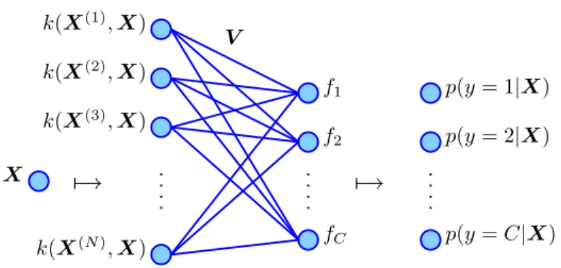
p(y=i|X,V) = e vTik(X) PC j=1e vT jk(X) fori= 1, . . . , C, (2.80) where k(X) = [k(X(1),X), . . . , k(X(N),X)]T is an N-dimensional vector consisting of the kernels computed between X and each training feature X(n). The kernel logistic regression model is illustrated in Figure 2.4.
2.2 Kernel Logistic Regression 25 V X f1 f2 fC p(y=C|X) p(y= 2|X) p(y= 1|X)
7→
7→
k(X(1),X) k(X(N),X) k(X(3),X) k(X(2),X)Figure 2.4: The kernel logistic regression model.
From equations (2.75), (2.76) and (2.80) above, we note that there are no explicit reference neither to the mapφnor the positive definite matrixΣ. The training of the kernel logistic regression model through minimization of the criterion ˇPlog
δ (V;D) in (2.75) can be carried out only with the quantities K, Γ, δ, and the training set labels {y(1), . . . , y(N)}. In the prediction of a new featureX, the weight matrix V and the vector k(X) of computed kernels between X and each training feature are needed. Note that the dimension that dominates the quantities needed in kernel logistic regression is the number of training examplesN, irrespective of the dimension of the underlying mappingφ. In practice, this allows for a very large dimension of the image of φas long as the kernelk can be efficiently computed. We will see in the next subsection that many such kernels and corresponding mappings exist.
In the following we will be concerned with the minimization of the criterion ˇPlog
δ (V;D) in (2.75) with respect to the dual parameter matrix V. An optimization algorithm will be presented that makes use of both the gradient and the Hessian of the criterion function, whose expressions are given in the following two lemmas.
Lemma 2.2.1 The gradient of (2.75) is theN ×C matrix
∇VPˇδlog(V;D) =K( ˇP(V)T−YT+δVΓ), (2.81) where Pˇ(V) =P(W) =P(Σ−1ΦV).
Proof See App. A
Lemma 2.2.2 The Hessian of (2.75) is
∇2 VPˇ log δ (V;D) = N X n=1 (diagp(n)−p(n)p(n)T)⊗k(X(n))kT(X(n)) +δΓ⊗K. (2.82)
Proof See App. A SincePlog
δ is convex with respect toW, andV is a linear transformation ofW, the criterion function ˇPδlog is convex with respect toV with a unique minimum that occurs for the minimizer
V∗ = 1 δ(Y
T−Pˇ(V∗)T)Γ−1. (2.83)
The above equation is the result of setting the gradient in (2.81) to zero. Note that V∗ in the equation above is the same as the one in (2.72), and hence the minimum obtained withV∗ is exactly the same as the minimum obtained with W∗. This means that we can obtain the same result by optimizing the criterion function with respect to the dual parameter matrix V instead of the primal parameter matrixW.
We will here present an optimization algorithm for estimating the weight matrix V that was introduced in [Tanabe, 2001a] where it was called the
dual penalized logistic regression machine (dPLRM). In this algorithm, the
weight matrix is updated iteratively using Newton’s method, where each step is
Vi+1 =Vi−αi∆Vi, (2.84) where ∆Vi is defined in
vec ∆Vi = [∇2VPˇδlog(Vi;D)]−1vec∇VPˇδlog(V
i;D). (2.85) As for the optimization of the penalized likelihood that was presented in the previous section, we compute an approximation to ∆Viusing the conjugate gradient (CG) method, since the inverse of the Hessian matrix is costly to obtain. This amounts to solving for ∆Vi in the equation
∇2 VPˇ log δ (V i;D) vec ∆Vi = vec∇ VPˇδlog(V i;D), (2.86) which after substitution of (2.81) and (2.82) reduces to
N
X
n=1
k(X(n))kT(X(n))∆Vi(diagp(n)−p(n)p(n)T) +δK∆ViΓ
=K( ˇP(ViT)−YT+δViΓ). (2.87) IfK is non-singular, we can pre-multiply both sides of the above equation withK−1, which yields
N
X
n=1
enkT(X(n))∆Vi(diagp(n)−p(n)p(n)T) +δ∆ViΓ
2.2 Kernel Logistic Regression 27
sinceK−1k(X(n)) =en, where e
n is the unit vector with all zeros except for thenth element which is 1.
The CG method for solving this equation is summarized in the follow-ing algorithm, which computes an estimate of the weight matrix V that minimizes the criterion ˇPlog
δ (V;D) in (2.75).
Algorithm 2.2.3 (The dual penalized logistic regression machine [Tan-abe, 2003])Start with an initial weight matrix V0 and generate a sequence of matrices according to
Vi+1=Vi−αi∆Vi, (2.89)
where ∆Vi is computed using the following conjugate gradient method:
1. Initialize: Start with an initial matrix∆V0i and compute the matrices
R0 and Q0: R0 = ˇP(ViT)−YT+δViΓ − N X n=1 enkT(X(n))∆V0i(diagp(n)−p(n)p(n)T)−δ∆V0iΓ, (2.90) Q0 =k(X(n))eTnR0(diagp(n)−p(n)p(n)T)−R0Γ. (2.91) 2. Iterate: Generate a sequence (∆V1i,∆V2i, . . .) according to
αj = k k(X(n))eTnRj(diagp(n)−p(n)p(n)T) +RjΓk2 kenk(X(n))TQj(diagp(n)−p(n)p(n)T) +QjΓk2 , (2.92) ∆Vji+1= ∆Vji+αjQj, (2.93) Rj+1= ˇP(ViT)−YT+δViΓ − N X n=1 enkT(X(n))∆Vji+1(diagp(n)−p(n)p(n)T)−δ∆Vji+1Γ, (2.94) βj+1 = k k(X(n))eTnRj+1(diagp(n)−p(n)p(n)T) +Rj+1Γk2 kk(X(n))eT nRj(diagp(n)−p(n)p(n)T) +RjΓk2 , (2.95) Qj+1=k(X(n))eTnRj+1(diagp(n)−p(n)p(n)T)−Rj+1Γ+βj+1Qj. (2.96)
2.2.1 The Kernel
A kernel is a symmetric function k : X × X → R. In kernel logistic
regression and other kernel methods, not all kernels are interesting. We focus our attention on kernels that are positive definite or conditionally positive definite, as given in the following definition.
Definition [Sch¨olkopf and Smola, 2002] LetX be a nonempty set. A real-valued symmetric function k : X × X → R is called a positive definite
kernel if for all N ∈ N and all X(1), . . . ,X(N) ∈ X the induced N ×N
kernel matrix K with elements k(X(m),X(n)) satisfies aTKa ≥ 0 given any vectora∈RN. The functionkis called aconditionally positive definite
kernel if K satisfies the above inequality for any vector a ∈ RN with
PN
n=1an= 0.
The following lemma relates the set of positive definite kernels and the set of conditionally positive definite kernels. We will be needing the lemma in Chapter 4 when we introduce a kernel for time series.
Lemma 2.2.4 ([Sch¨olkopf and Smola, 2002])
(i) Any positive definite kernel is also a conditionally positive definite kernel.
(ii) eβk is positive definite for all β > 0 if and only if k is conditionally positive definite.
Proof See [Sch¨olkopf and Smola, 2002].
The kernel defined in (2.79) is positive definite since we requireΣ, and thereby Σ−1, to be a positive definite matrix. Note that this kernel can be written as an inner product between two vectors ψ(X) and ψ(X0) by letting ψ(X) =Σ−1/2φ(X;λ). That is,
k(X,X0) =ψT(X)ψ(X0), (2.97) where the mapping ψ :X →RM+1 is defined in terms of the mapping φ
and the positive definite matrix Σ. Now, it follows from Mercer’s Theo-rem [Mercer, 1909; Sch¨olkopf and Smola, 2002] that any positive definite
kernel admits the form of an inner product ψT(X)ψ(X0) for some map-ping ψ. Therefore, instead of choosing ψ explicitly through choices of φ and Σ, we could choose a positive definite kernel k that implicitly defines a mapping ψ, which in turn implicitly defines φ and Σ. Then, with the choice of a kernel k, the dual parameter matrix V can be estimated by
2.2 Kernel Logistic Regression 29
minimizing the criterion ˇPlog
δ (V;D) in (2.75), and the conditional proba-bilityp(y=i|X,V) in (2.80) can be computed, without explicitly defining φand Σ. Herein lays the elegance and power of kernel logistic regression, and more generally kernel methods. By choosing a positive definite kernel k, there exists a mapping ψ that maps the features into a possible infi-nite dimensional space, where linear prediction is performed. Moreover, depending on the choice of kernel, learning algorithms can run on a com-puter in a small amount of time and generate complex nonlinear classifiers that would be extremely difficult or even impossible using only the primal method of logistic regression.
As an example, let the observation space be X =RD and consider the
polynomial kernel
k(x,x0) = (xTx0+ 1)d, (2.98) wherex,x0 ∈RD and dis a positive integer. The corresponding mapping
ψmaps each vectorxinto the space of all monomials up to degree dof its elements. This is the space where linear prediction is performed. The inner product of two mapped vectors is efficiently computed through the kernel in (2.98).
Another example of a kernel for X =RD is theGaussian kernel
k(x,x0) =e−
||x−x0||2
2σ2 , (2.99)
wherex,x0 ∈RD and σ >0. The image of the associated mapping ψ has
infinite dimension.
The design of kernels for more complex setsX is an important research topic. Two general design methodologies are 1) to construct a kernel from generative models (e.g., [Jaakkola and Haussler, 1999a]), and 2) to con-struct a kernel from a similarity measure (e.g., [Vert et al., 2004]). In Chapter 4 we will present various kernels for time series extracted from speech signals using both of the above design methodologies.
2.2.2 Sparse Approximations
In KLR, we need to store all theN inputsX(1), . . . ,X(N), since they are needed in the classification of a new example X according to (2.80). We also need to store the (N×C)-dimensional dual parameter matrixV. IfN is large, which is the case for many practical problems, the memory require-ments and computational complexity may become impractically large. In many applications in automatic speech recognition, for example, the num-ber of training examples can be several hundreds of thousands.
A way to overcome the above problem is to select only a small repre-sentative subset S of the training data for inclusion in the kernel logistic
regression model. In [Zhu and Hastie, 2001, 2005; Myrvoll and Matsui, 2006], the authors presented a greedy training algorithm for KLR. The algorithm is greedy in the sense that it starts with an empty set S, and incrementally adds additional training examples to S based on which ex-amples improve the criterion function the most. The subset is increased until convergence. The size of the obtained subset is typically smaller than the number of support vectors in the support vector machine (SVM) [Zhu and Hastie, 2001, 2005].
The approach taken in [Krishnapuram et al., 2005] is to use a sparse-promoting Laplacian prior instead of a Gaussian prior typically assumed for KLR. The price we have to pay for using a Laplace prior instead of a Gaussian prior, is a criterion function that is no longer differentiable. The authors in [Krishnapuram et al., 2005] propose to optimize a smooth bound on the criterion function instead of the original criterion function, in a similar fashion as the celebrated expectation maximization (EM) algorithm [Dempster et al., 1977]. The result is that many of the training examples will have zero weights and can therefore be omitted in the KLR model.
2.3
Summary
In this chapter, we presented the framework of logistic regression in the con-text of multiclass classification. Both penalized logistic regression (PLR) and kernel logistic regression (KLR) were considered. The logistic regres-sion framework we presented is general in the sense that it can be applied to any kind of data. In particular, in the rest of this thesis we will consider the application of logistic regression to speech recognition, where the in-puts are sequences of vectors. Two new concepts that we introduced were adaptive regressor parameters and garbage class. We will have more to say about these concepts in the context of speech recognition in the following chapters.
As a final note, we would like to make clear that KLR is very similar to Gaussian process (GP) classification [Williams and Barber, 1998; Jaakkola and Haussler, 1999b; Rasmussen and Williams, 2006]. The difference lies in that GP classification is a fully Bayesian approach, meaning that the pos-terior distribution of the parameters is used in prediction, while KLR only uses the MAP estimate of the parameters. The fully Bayesian approach has to deal with an analytically intractable integral that can only be eval-uated numerically. Several methods exist, one of which uses the Laplace approximation [Williams and Barber, 1998].
Chapter 3
Speech Recognition and
Hidden Markov Models
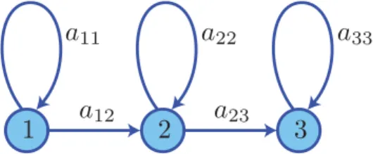
The hidden Markov model (HMM) is a powerful model for sequences of variable lengths. It has been well studied over the last few decades for automatic speech recognition applications. This chapter gives an overview of the HMM and its use in automatic speech recognition. We will make use of the HMM in subsequent chapters due to its strengths in sequence modeling.
There are generally two ways to explain the HMM. The first approach explains the HMM as a model for generating sequences of observations. The most prominent example of this approach is [Rabiner, 1989], which explains the HMM using a simple example concerning the generation of a sequence of colored balls from a set of urns each containing a different distribution of colored balls. The second approach is more probabilistic in the sense that it explains the HMM as a probability distribution over sequences. Examples of the latter approach are [Bilmes, 2006; Jordan, 2007]. The presentation in this chapter uses the latter approach.
We start by presenting the usual way of extracting a sequence of feature vectors from a speech signal. Then, in Section 3.2 we explain the HMM. Sections 3.3 and 3.4 concern the typical application of HMMs to isolated-word speech recognition and continuous speech recognition, respectively. Finally, Section 3.5 contains a short summary of the chapter.
3.1
Feature Extraction
In automatic speech recognition, it is common to extract a set of features from each speech signal. Classification is carried out on the set of features instead of the speech signals themselves. A good set of features should
Figure 3.1: Feature extraction from a speech signal.
include discriminative information and exclude information that is irrele-vant for classification (e.g., speaker dependent information such as pitch). Moreover, the feature set should be small enough to allow fast processing and robust.
A speech signal can be considered to be a realization of a short-time stationary stochastic process. This means that although the statistical
characteristics of a speech signal change over time, they can be considered to be stationary within small time intervals (20-30 ms). This observation, together with the observation that the most prominent discriminative in-formation between speech signals appear in the frequency domain, has lead to the common approach of extracting a time series which is a sequence of short time spectral feature vectors from each speech signal.
Figure 3.1 illustrates the extraction of a time series X = (x1, . . . ,xT) from a speech signal. A window function of fixed width (often a Hamming window of width 20-30 ms) is used to confine processing to a short-time segment of the speech signal in order to generate a spectral feature vector. The window function is shifted a fixed length in time (typically 5-10 ms) to the right for further extraction of feature vectors until the end of the speech signal is reached.
Note that since different speech signals have different durations, feature extraction with a fixed window shift leads

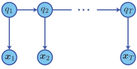
![Figure 3.2 illustrates the HMM as a graphical model [Jordan, 2007].](https://thumb-us.123doks.com/thumbv2/123dok_us/773815.2597866/44.748.259.544.505.617/figure-illustrates-hmm-graphical-model-jordan.webp)