Ensemble projection for semi-supervised Image classification

(1)

Ensemble Projection for Semi-supervised Image Classification

Dengxin Dai

Computer Vision Lab, ETH Zurich

[email protected]

Luc Van Gool

Computer Vision Lab, ETH Zurich

[email protected]

Abstract

This paper investigates the problem of semi-supervised classification. Unlike previous methods to regularize clas-sifying boundaries with unlabeled data, our method learns a new image representation from all available data (labeled and unlabeled) and performs plain supervised learning with the new feature. In particular, an ensemble of image pro-totype sets are sampled automatically from the available data, to represent a rich set of visual categories/attributes. Discriminative functions are then learned on these proto-type sets, and image are represented by the concatenation of their projected values onto the prototypes (similarities to them) for further classification. Experiments on four standard datasets show three interesting phenomena: (1) our method consistently outperforms previous methods for semi-supervised image classification; (2) our method lets it-self combine well with these methods; and (3) our method works well for self-taught image classification where unbeled data are not coming from the same distribution as la-beled ones, but rather from a random collection of images.

1. Introduction

Providing efficient solution to image classification has always been a major focus in computer vision. Most of the classification systems [3, 17] heavily rely on manually la-beled training data, which is expensive and sometimes im-possible to acquire. The scarcity of annotations, combined with the explosion of image data, has shifted focus towards learning with less supervision. As a result, numerous tech-niques such as semi-supervised learning [10], active learn-ing [12], transfer learnlearn-ing [24], and self-taught learnlearn-ing [25] have been developed.

In this paper, we are interested in the problem of semi-supervised learning (SSL) for image classification. The task is to design a method that can make use of unlabeled im-ages, while learning classifiers from labeled ones. Recent research in SSL has obtained some success in solving this problem [10, 18, 21]. Most of these methods build

them-selves upon thelocal-consistencyassumption that data

sam-ples with high similarity should share the same label. This assumption allows the geometrical structure of unlabeled data to regularize the classifying functions. While improve-ments have been reported, these methods share three com-mon drawbacks.

First of all, these methods only exploit the

local-consistencyassumption in image feature space, and ignore other prior information. Another reasonable assumption -borne out by our results - is that samples with very low sim-ilarity are in high probability come from different classes.

We call this the exotic-inconsistencyassumption, and

de-sign a method to exploit it also for SSL. Furthermore, most previous methods design specialized learning algorithms to leverage the structure of unlabeled data [2, 15, 18], so users often need to change their learning methods in order to uti-lize the cheap unlabeled data. This limits the applicability of SSL, as users usually are reluctant to give up their fa-vorite classifiers. Last but not the least, previous methods assume that the unlabeled data are coming from more or less the same distribution as the labeled data. This imposes restrictions as well, as many applications have no prior ac-cess to the data to be classified. To overcome these limita-tions, we depart from the traditional paradigm and propose another route to SSL in this paper. Below, we present our motivations and outline the method.

People learn and generalize object classes well from their characteristics, such as color, texture, and size. We also do so by comparing an object with other objects in the world. This is part of Eleanor Rosch’s prototype the-ory [27], that states that an object’s class is determined by its

similarityto prototypes which represent object categories. The theory is suitable for transfer learning [24], where la-beled data of other categories are available. An important question is whether the theory can also be used for SSL, with its huge amount of unlabeled data. Our paper investi-gates this problem.

To use this paradigm, we first need to create the pro-totypes automatically from unlabeled data. Based on the

local-consistencyand theexotic-inconsistencyassumptions, it stands to reason that samples along with their closest 2013 IEEE International Conference on Computer Vision

(2)

Known data Sampling An image Projection function 1 Projecting Concat-enating vector T Projection function T Vector 1 Projection vector Training 1 2 3 1 2 3 Prototype set T Prototype set 1 Labeled Unlabeled Labeled images Car Cow Training Classifiers Car

Feature learning Classification with the learned feature ...

...

An unlabeled image

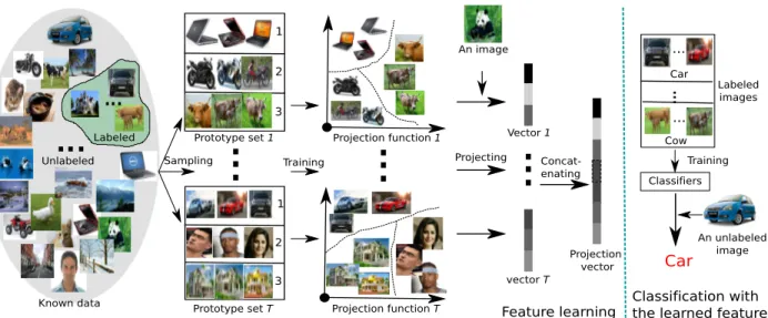
Figure 1. The pipeline of Ensemble Projection (EP). EP consists in unsupervised feature learning (left panel) and plain supervised classifica-tion (right panel). For feature learning, we sample an ensemble ofTdiverse prototype sets from all known images and learn discriminative classifiers on them for the projection functions. Images are then projected using these functions to obtain their new representation. For classification, we train plain classifiers on labeled images with the learned features to classify the unlabeled ones.

neighbors can be “good” prototypes (defining one visual category/attribute), and far apart such prototypes can play the role of different categories. According to this observa-tion, we design a method to sample the prototype set from all available data. Discriminative learning is then used, lo-gistic regression in our implementation, to learn projection functions tuned to the prototypes. Images are linked to the prototypes via their projection values (classification scores). Since information carried by one single prototype set is lim-ited and can be noisy, we borrow ideas from ensemble learn-ing [26] to create an ensemble of diverse prototype sets, which in turn leads to an ensemble of projection functions. Images are then represented by the concatenation of their projected values (similarities) to all the image prototypes, in keeping with prototype theory [27]. We call the method Ensemble Projection (EP) and it is illustrated in Fig. 1.

Solving SSL problems this way, EP addresses all the

three aforementioned issues: (1) in addition to

local-consistency property, it also exploits exotic-inconsistency

property; (2) the learned new feature can be fed into any classifiers; and (3) it performs well for self-taught image classification, supported by experiments. Our contributions

are: (1) theexotic-inconsistencyassumption and solving the

SSL task as a feature learning problem; (2) a simple, yet effective way to create an ensemble of diverse prototype sets; (3) experimental verification that our method is supe-rior to competing methods, combines well with them, and is more generally applicable. While we focus in this paper on image classification, our framework is fairly general: the framework can be used for other tasks as well, such as clus-tering and retrieval. The code of this work is available at

www.vision.ee.ethz.ch/˜daid/EnPro.

The rest of this paper is organized as follows. Sec.2 re-ports on related work. Sec.3 describes our approach, fol-lowed by experiments in Sec.4. Sec.5 concludes the paper.

2. Related Work

Our method is generally relevant to semi-supervised learning, ensemble learning, and image feature learning.

Semi-supervised Learning. There is a large body of work on semi-supervised learning (SSL) [35]. SSL aims at enhanced learning by exploiting available, unlabeled data. One group of methods is based on label propaga-tion over a graph, where nodes represent data examples and edges reflect their similarities. The optimal labels are those that are maximally consistent with the supervised class labels and the graph structure. Well known exam-ples include Harmonic-Function [34], Local-Global Con-sistency [33], Manifold Regularization [1], and Engenfunc-tion [10]. While having strong theoretical support, these methods cannot label unseen data. Another group of meth-ods utilize the unlabeled data to regularize the classifying functions – enforcing the boundaries to pass through re-gions with a low density of data samples. The most no-table methods are transductive SVM [13], Semi-supervised SVM [2], and semi-supervised random forest [18]. Read-ers are referred to [35] for a thorough overview of SSL.

For semi-supervised image classification, Guillaumin et

al. [11], and Shrivastavaet al. [29] presented two methods

in the self-supervised manner – unlabeled images with high classification confidence are then included into the training set for the next round of learning. While obtaining promis-ing results, they both require additional supervision: [11]

(3)

needs image tags and [29] image attributes.

Ensemble Learning. Our method learns the represen-tation from an ensemble of prototype sets, thus sharing as-pects of ensemble learning (EL). EL builds a committee of base learners, and finds solutions by maximizing the agree-ment. Popular ensemble methods that have been extended to semi-supervised scenarios are Boosting [15] and Ran-dom Forest [18]. However, these methods still differ signif-icantly from ours. They focus on the problem of improving classifiers by using unlabeled data. Our method learns new representations for images using all data available. Thus, it is independent of the classification methods. The reason we use EL is to capture rich visual attributes from a series of prototype sets. Other work close to ours is that of Dai

et al. [5]. They presented an ensemble partitioning frame-work for unsupervised image categorization, where weak training sets are sampled to train base learners. The whole dataset is classified by all the base learners in order to obtain a bagged proximity matrix for further clustering. A similar idea was also proposed in Random Ensemble Metrics [14], where images are projected to randomly subsampled train-ing categories for supervised distance learntrain-ing.

Feature Learning. Over the past years, a wide spec-trum of features, from pixel-level to semantic-level, have been designed and used for different vision tasks. Due to the semantic gap, recent work builds up high-level features, which go beyond single images and are probably impreg-nated with semantic information. Notable examples are Im-age Attributes [8], Classemes [30], and Object Bank [19]. While getting pleasing results, these methods all require additional labeled training data, which is exactly what we want to avoid. There have been several attempts [28, 32] to avoid the extra attribute-level supervision, but they still re-quire canonical category-level supervision. Our representa-tion learning is fully unsupervised. The method also shares similarity with Self-taught learning [25], where sparse cod-ing is employed to construct higher-level features uscod-ing un-labeled data. Both work attempt to leverage the regularities of general visual data to improve image representation.

3. Our Approach

The training data consists of both labeled data Dl =

{(xi, yi)}li=1and unlabeled dataDu = {xj}lj+=ul+1, where

xi denotes the feature vector of imagei,yi ∈ {1, ..., K}

is its label, andKis the number of classes. Most previous

semi-supervised learning (SSL) methods learn a classifier

φ : X 7→ Y fromDlwith a regulation term learned from

Du. Our method learns a new image representationf from

all known dataD = Dl∪ Du, and train plain classifierφ

onf. fiis a vector of similarities of imageito a series of

sampled image prototypes.

Assume that EP learns knowledge fromTprototype sets

Pt,t∈{1,...,T} ₌ _{₍_st

i, cti)}rni=1, where sti ∈ {1, ..., l+u}

is the index of theithchosen image,ct_i ∈ {1, ..., r}is the

pseudo-label indicating which prototypest_i belong to. ris

the number of prototypes (analogous to the number of

ob-ject classes) inPt_{, and}_n_{the number of images sampled for}

each prototype (e.g.r = 3andn = 3in Fig. 1). Below,

we first present our sampling method of creating a single

prototype setPt_{in the}_t_{trial, followed by EP.}

3.1. Max-Min Sampling

As stated, we want the prototypes to be inter-distinct and intra-compact, so that each one represents a different visual concept. To this end, we design a 2-step sampling method, termed Max-Min Sampling. The Max step is designed for the inter-distinct property, and the Min-step for the intra-compact one. In particular, we first sample a skeleton of the prototype set, by looking for image candidates that are strongly spread out, i.e. at large distances from each other. We then enrich the skeleton to a prototype set by includ-ing the closest neighbors of the skeleton images. The

al-gorithm for creatingPt_{is given in Algo.1. For the}

skele-ton, we randomly sampledmhypotheses – each hypothesis

consists ofr random sampled images – and keep the one

having the largest mutual distance. This simple procedure guarantees that the sampled seed images are far from each other. Once the skeleton is created, the Min-step extends each seed image to an image prototype by introducing its

nnearest neighbors (including itself), in order to enrich the

characteristics of each image prototype and reduce the risk of introducing noisy images. The pseudo-labels are shared by all images specifying the same prototype. It is worth pointing out that the randomized Max-step may not gen-erate the optimal skeleton. However, it serves its purpose well. For one thing, we do not need the optimal one – we

only need the prototypes to befar apart, notfarthest apart.

Moreover, the randomized step leaves room for randomness so that diverse visual concepts can be captured in different

Pt_{’s. The dis}₍_{., .}₎_{in line}₅_{represents the distance between}

two visual vectors,L1distance metric in our

implementa-tion.

3.2. Ensemble Projection

We now explore the use of the image prototype sets

cre-ated in§3.1 for a new image representation. Because the

prototypes are compact in feature space, each of them im-plicitly defines a visual concept (image attribute). This is

es-pecially true when the datasetDis sufficiently large, which

is to be expected given the vast numbers of unlabeled im-ages that are available. Since information carried by a single

prototype setPt_{is quite limited, we borrow idea from}

en-semble learning (EL) to create an enen-semble ofTsuch sets.

As we all know, EL benefits from the precision of its base learners and their diversity. For good precision,

(4)

Algorithm 1:Max-Min Sampling intth_trial

Data: DatasetD

Result: Prototype setPt 1 begin

2 ˆe= 0; /* Max-step */

3 whileiterations≤mdo

4 V={rrandom image indexes};

5 e=P i∈V P j∈Vdis(xi,xj); 6 if e >eˆthen 7 ˆe=e; 8 Vˆ=V; 9 end 10 end 11 fori←1tordo /* Min-step */ 12 st

i=indexes of thennearest neighbors ofV(i)inD; 13 ct_i= (i, i, ..., i)∈_Rn; 14 end 15 st_{= (}_st 1, ...,str)∈Rrn; /* Constructing Pt */ 16 ct= (ct₁, ...,ct_r)∈_Rrn; 17 Pt={(st_i, ct_i)}rn_i₌₁; 18 end

logistic regression is used in our implementation to project

each input imagexto the image prototypes to measure the

similarities. For large diversity, randomness is introduced in different trials of Max-Min Sampling to create an ensem-ble of diverse prototype sets, so that a rich set of image at-tributes are captured. The vector of all similarities is then

concatenated and used as a new image representationf for

the final classification. A plain classifier (e.g. SVMs and

boosting) can then be trained onDlfor our semi-supervised

classification, as unlabeled data has already been explored

in obtainingf. The whole procedure of EP is presented in

Algo.2. Up to now, the whole pipeline in Fig.1 has been explained.

4. Experiments

Datasets: We evaluated our method on four datasets:

Scene-15(S-15) [17], LandUse-21 (L-21) [31], Texture-25

(T-25) [16], and Caltech-101(C-101) [9]. Scene-15dataset

contains15scene categories with both indoor and outdoor

environments,4485images in total. Each category has200

to 400 images. LandUse-21 consists of satellite images

from 21categories, 100 images each. Texture-25 dataset

contains25texture categories, 40samples each.

Caltech-101 contains101 object categories, 8677 images in total,

and each one has31to800images. Furthermore, we

col-lected a random image collection by sampling20,000

im-ages randomly from ImageNet dataset [6] to evaluate our method on the task of self-taught image classification. Since

the current version of ImageNet has already had 21841

synsets (categories) and more than14 millions of images

in total, the chance is vanishingly small that images of the random image collection and images of the four datasets

Algorithm 2:Ensemble Projection

Data: DatasetD,an input imagexi

Result: Projected representationfi 1 begin

2 fort←1toTdo

3 SamplePt={(s_it, ct_i)}rn_i₌₁using Algo. 1 ; 4 Train classifiersφt(.)∈ {1, ..., r}onPt; 5 Obtain projection vector:ft

i =φt(xi); 6 end

7 fi= ((fi1)>, ...,(fiT)>)>; 8 end

considered are coming from the same distribution.

Features:The following three features were used in our experiments: GIST [23], Pyramid of Histogram of Ori-ented Gradients (PHOG) [3], and Local Binary Patterns (LBP) [22]. GIST was computed on the rescaled images

of256×256pixels, in4,8 and8orientations at3 scales

from coarse to fine. PHOG was computed with a2-layer

pyramid and in8directions. For LBP, the uniform LBP was

used. These features were used due to their low dimension, as our method requires ‘meaningful’ neighborhoods to ex-ploit.

Competing methods: Four classifiers were adopted to evaluate the method, with two inductive classifiers logis-tic regression (LR) and linear SVMs, and two transduc-tive classifiers Harmonic-Function (HF) [34] and LapSVM (LSVM) [1]. HF formulates the SSL learning problem as a Gaussian Random Field on a graph for label propagation. LapSVM extends SVMs by including a smoothness penalty term defined on the Laplacian graph. Since our method builds up a new feature representation, we illustrate the per-formance of all methods working with normal features and our learned features.

Experimental settings: We conducted five sets of ex-periments: (1) compare our method with competing meth-ods for semi-supervised image classification, where the un-labeled images are from the same categories as the un-labeled ones; (2) evaluate the robustness of our method against its parameters; (3) evaluate the robustness of our method against the choices of different image features; (4) evaluate the robustness of the method against classifier models; and (5) evaluate the performance of our method for the task of self-taught image classification. For all experimental sets except (4), the same set of parameters were used for all the classifiers. We used L2-regularized LR of LIBLINEAR [7]

withC = 15 and the linear SVMs of LIBSVM [4] with

C = 15. For LapSVM, we used the scheme suggested

by [1]: γA was set as the inductive model,10in our case,

andγI was set as₍_l₊γI_ul₎2 = 100γAl.

As to features, while Algo. 1 and Algo. 2 use the same

notationx, we used GIST for Algo. 1 and the

(5)

1 2 5 10 20 50 100 20 30 40 50 60 70 80

Number of labeled images per class

MAP (%) LR LR+EP SVMs SVMs+EP HF LSVM 1 2 5 10 20 30 50 10 20 30 40 50 60 70 80

MAP (%) LR LR+EP SVMs SVMs+EP HF LSVM 1 2 5 10 15 20 30 10 20 30 40 50 60 70 80 90

MAP (%) LR LR+EP SVMs SVMs+EP HF LSVM 1 2 5 10 15 20 30 5 10 15 20 25 30 35

MAP (%) LR LR+EP SVMs SVMs+EP HF LSVM 1 2 5 10 20 50 100 30 40 50 60 70 80

MAP (%) LR+EP HF HF+EP LSVM LSVM+EP 1 2 5 10 20 30 50 20 30 40 50 60 70 80

MAP (%) LR+EP HF HF+EP LSVM LSVM+EP 1 2 5 10 15 20 30 20 30 40 50 60 70 80 90

MAP (%) LR+EP HF HF+EP LSVM LSVM+EP 1 2 5 10 15 20 30 5 10 15 20 25 30 35

MAP (%) LR+EP HF HF+EP LSVM LSVM+EP

Scene-15 LandUse-21 Texture-25 Caltech-101

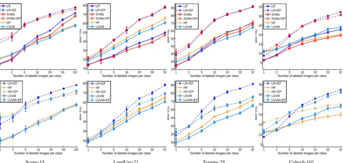
Figure 2. Semi-supervised classification results on the four datasets. The top panel evaluate the performance of our learned features when fed into LR and SVMs. The bottom shows its performance when fed into HF [34] and LapSVM [1]. All methods were tested with two feature inputs: the concatenation of GIST, PHOG and LBP, and our learned feature from them (indicated by “+ EP”).

Methods LR LR + EP SVMs SVMs + EP HF [34] HF + EP LSVM [1] LSVM + EP S-15 38.6 (1.6) 61.3 (1.9) 36.6 (2.8) 60.8 (2.3) 37.5 (2.4) 59.6 (2.0) 37.2 (2.1) 57.1 (2.2) L-21 24.2 (1.2) 41.0 (0.8) 23.1 (1.1) 41.6 (0.6) 34.8 (1.4) 37.7 (1.7) 32.4 (1.2) 37.9 (2.0) T-25 36.2 (2.5) 57.9 (2.5) 34.4 (2.1) 58.2 (2.6) 38.9 (0.6) 50.9 (2.2) 34.0 (1.2) 51.0 (2.0) C-101 14.0 (0.2) 19.1 (0.4) 12.7 (0.1) 19.9 (0.2) 14.4 (0.3) 20.0 (0.4) 15.0 (0.3) 21.0 (0.5)

Table 1. MAP of semi-supervised classification on the four datasets, with5training examples per class. All methods were tested with two feature inputs: the concatenation of GIST, PHOG, and LBP, and our learned feature from it (indicated by “+ EP”)

Algo. 1 needs a low dimensional feature to define neighbor-hoods, while Algo. 2 needs a discriminative feature to learn precise projection functions. Experimental set (3) was con-ducted by providing the same single feature to Algo. 1 and Algo. 2. As to the parameters of our method, we used the

following for experimental sets (1), and (3)–(5): T = 300,

r= 30,n= 6, andm = 50. A wide variety of values for

them were tested in experimental set (2). For all the

exper-iments, we performKrounds of binary classification, each

time taking one class as positive and the rest as negative, as LapSVM only work for two-class cases. Multi-class aver-age precision (MAP) was used as the evaluation criteria: the average precision over all recall values and over all classes.

4.1. Semi-supervised Image Classification

In this section, we evaluate all methods across

all datasets for semi-supervised image classification.

Different numbers of training images per category

were tested: Scene-15 with {1,2,5,10,20,50,100},

LandUse-21 with {1,2,5,10,20,30,50}, Texture-25

with {1,2,5,10,15,20,30}, and Caltech-101 with

{1,2,5,10,15,20,30}. In all cases, the rest images were

taken as unlabeled training data (also used for evaluation).

The reported results are the average performance over 5

runs with random labeled-unlabeled splits.

Fig. 2 shows all the results and Table 1 lists the results

obtained with5labeled training images per class. From the

top panel of Fig. 2, it is easy to observe that the two plain classifiers LR and SVMs working with our feature perform better than the two sophisticated SSL methods LapSVM and Harmonic-Function working with the original feature, while having comparable variance. This suggests that our method can achieve promising results for semi-supervised image classification, even combined with plain classifiers. The advantages can be ascribed to two factors: (1) in

addi-tion to thelocal-consistencyassumption, our method also

exploits the exotic-inconsistency assumption; (2) the

dis-criminative projections abstract high-level attributes from

the sampled prototypes,e.g. owning “yellow-smooth” more

than “dark-structured”. As already proven in fully super-vised scenarios [8, 24], prototype-linked, attribute-based features are very helpful for image classification. Note that our feature are learned exactly from the original feature, but going beyond one single image.

We further investigate the complementarity of our learned feature and other SSL methods for semi-supervised classification. It is interesting to see from the bottom panel

(6)

2 5 10 50 100 300 10 20 30 40 50 60 70

The number T of prototype sets

MAP (%) Scene−15 LandUse−21 Texture−25 Caltech−101 2 5 10 20 30 50 10 20 30 40 50 60 70

The number r of prototypes in each set

MAP (%) Scene−15 LandUse−21 Texture−25 Caltech−101 1 2 5 10 20 30 50 20 30 40 50 60 70 80

The number n of images in each prototype

MAP (%) Scene−15 LandUse−21 Texture−25 Caltech−101 5 10 50 100 200 500 20 30 40 50 60 70 80

The number of skeleton hypotheses m

MAP (%)

Scene−15 LandUse−21 Texture−25 Caltech−101

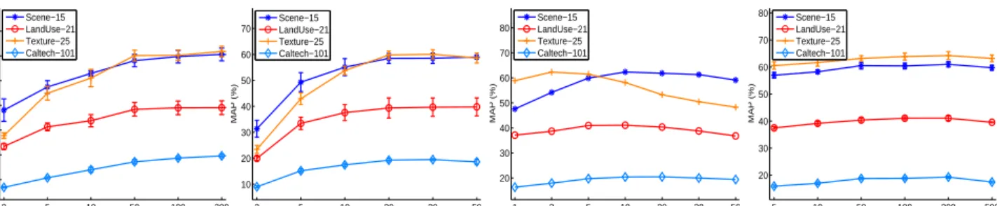
Figure 3. Performance of our method as a function ofT,r,n, andm. LR was employed with5labeled training images per class.

1 2 5 10 20 50 100 10 20 30 40 50 60 70 80

Number of training images per class

MAP (%) GIST EP (GIST) PHOG EP (PHOG) LBP EP (LBP) 1 2 5 10 20 30 50 10 20 30 40 50 60 70 80 90

MAP (%) GIST EP (GIST) PHOG EP (PHOG) LBP EP (LBP) 1 2 5 10 15 20 30 10 20 30 40 50 60 70 80 90 100

MAP (%) GIST EP (GIST) PHOG EP (PHOG) LBP EP (LBP) 1 2 5 10 15 20 30 0 5 10 15 20 25 30 35 40

MAP (%) GIST EP (GIST) PHOG EP (PHOG) LBP EP (LBP)

Figure 4. Comparison of our learned features (indicated by EP(.)) to the corresponding original features GIST, PHOG, and LBP . LR was used as the classifier with5labeled training images per class.

of Fig. 2 and Table 1 that combining the two boosts the per-formance also. This suggests that our scheme of exploiting unlabeled data and the previous ones doing so capture com-plementary information. The increase is more pronounced for Harmonic-Function (HF) than for LapSVM. This is in line with our intuitive understanding that HF’s underlying technique label propagation on Gaussian Random Fields is more complementary to our technique discriminative learn-ing on image neighborhoods.

4.1.1 Robustness Against Parameters

In this section, we examine the influence of the parameters of our method on classification performance. They are the

total number of prototype setsT, the number of prototypes

in each set r, the number of images in each prototype n,

and the number of skeleton hypothesesmused in Max-Min

Sampling. LR was used as the classifier here. The param-eters were evaluated in the following way – each time the value of one changes while the others being fixed to the val-ues described in the experimental settings.

Fig. 3 shows the results over a range of their values. The figure shows that the performance of our method increases

pretty fast withT, but then stabilizes quickly. It implies that

the method benefits from exploiting more “novel” visual

attributes (image prototypes). After T increases to some

threshold (e.g.50for the four datasets), the then exploited

attributes have already been in, thus stopping boosting the

performance much. Forr, the figure shows that the

perfor-mance generally increases with it. This is because a larger

leads to a precise attribute assignment, as a thorough

com-parison is performed. However, we found that whenrgoes

over20, the increase is not worth the computing time. A

largerwould lead to confusing attributes, because

proto-types may start overlapping with each other. Forn, a

simi-lar trend was obtained – asnincreases, the characteristics of

the prototypes are enriched, thus boosting the performance.

But beyond some threshold (e.g. 10 in our experiments),

more noisy images are introduced, thus degrading the

per-formance. For m, Fig. 3 shows that an undue large one

degrades the performance. This can be explained from the perspective of ensemble learning (EL). EL benefits from the strength of its base learners and their diversity. Too large an

mbrings all prototype skeletons close the the optimal one,

thus decreasing the diversity of sampled prototype sets. Although the performance of EP will be affected by the choice of its parameters, we can see from Fig. 3 that each of the parameters has a wide range of reasonable values to choose from. It is not difficult to choose a set of parameter values that produce better results than competing methods

(c.f. Fig. 3 and Table 1). Also, the parameters are quite

in-tuitive and their roles are similar to the parameters of some

principled methods, e.g. analogues of m,n andT can be

found in RANSAC,k-NN, and Bagging, respectively.

4.1.2 Robustness Against Features

In this section, we elaborate the performance of our method by using different single image features, in order to see its robustness against different feature choices. The LR was

(7)

1 2 5 10 20 50 100 20 30 40 50 60 70 80

MAP (%) LR LR+EP SVMs SVMs+EP 1 2 5 10 20 30 50 10 20 30 40 50 60 70

MAP (%) LR LR+EP SVMs SVMs+EP 1 2 5 10 15 20 30 10 20 30 40 50 60 70 80 90

MAP (%) LR LR+EP SVMs SVMs+EP 1 2 5 10 15 20 30 5 10 15 20 25 30 35

MAP (%)

LR LR+EP SVMs SVMs+EP

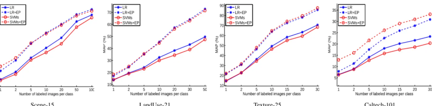
Figure 5. Self-taught classification results on the four datasets. The classifiers were tested with two feature inputs: the concatenation of GIST, PHOG, and LBP, and our learned feature from it (indicated by “+ EP”).

0.01 0.1 1 5 15 50 200 0 10 20 30 40 50 60 70 80 90 100 Parameter C MAP (%) Scene−15 Scene−15 (EP) LandUse−21 LandUse−21 (EP) Texture−25 Texture−25 (EP) Caltech−101 Caltech−101 (EP)

Figure 6. Comparison of our learned feature with the normal image feature against different LR models.

again used as the classifier and we compared our learned feature with the corresponding original ones, namely the GIST, the PHOG, and the LBP. The results in Fig. 4 show that all the learned features perform consistently better than the original ones, suggesting EP is robust against the choices of image features.

4.1.3 Robustness Against Classifier Models

In this section, we evaluate the robustness of our learned features against classifier models. Different values of the

error-margin balancing parameterCwere tested for LR and

SVMs. 5 labeled training examples per class were used.

A set of values{0.01,0.1,1,5,15,50,200}were tested for

theC of the SVMs and LR. The results of SVMs are not

affected by the changes of C, probability because SVMs

clearly separate the small number of training examples. Thus we only show the results of LR in Fig. 6. The figure shows that our feature consistently outperforms the origi-nal one over different classifier models. This property is important for SSL, as labeled data is limited and probably cannot accommodate a model selection technique such as Cross-Validation.

4.2. Self-taught Image Classification

In order to evaluate the applicability of our method, we tested it in a more general scenario, where the unlabeled

data is the set of20,000 random images from ImageNet.

Projection functions were learned from images in this set plus the labeled training images in corresponding evalua-tion dataset, and performance was measured on the unla-beled images. Fig. 5 shows the classification performance with different numbers of labeled training images per class,

and Table 2 lists that when5 training images per class is

used. From the figure and table, it can be found that our learned feature from the random image collection still out-performs the original feature. This property is important for semi-supervised learning, as it is often the case that one has no prior access to the data to be classified. The suc-cess could be ascribed to the fact that the “universal vi-sual world” (the random image collection) contains abun-dant high-level, valuable visual attributes such as “blue and open” in some image clusters and “textured and man-made” in others. Exploiting these “hidden” visual attributes is very beneficial for narrowing down the semantic gap between low-level features and high-level classification tasks.

From the figure, we can also find that as the number of labeled training images increases, the advantage of our learned feature may decrease. It comes without much sur-prise as the method is designed to improve classification systems by exploiting ‘unknowledgeable’ (unlabeled) data. Therefore, when a sufficient number of labeled images are available, introducing additional unlabeled ones may hurt

the system. This is a general, open problem for

semi-supervised learning (self-taught learning) [20]. One pos-sible solution is to study when the classification systems should switch from semi-supervised learning to fully super-vised learning.

5. Conclusion

This paper has tackled the problem of semi-supervised image classification from a novel perspective – rather than regularizing classifying functions like previous methods, we learn a new, high-level image representation. We

pro-posed as novel concept theexotic-inconsistencyassumption

and designed a simple, yet effective feature learning method

(8)

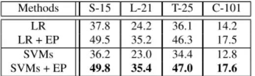
avail-Methods LR LR + EP SVMs SVMs + EP S-15 37.8 49.5 36.2 49.8 L-21 24.2 35.2 23.0 35.4 T-25 36.1 46.3 34.4 47.0 C-101 14.2 17.5 12.8 17.6

Table 2. MAP of self-taught classification, with5training exam-ples per class. All methods were tested with two feature inputs: the concatenation of GIST, PHOG, and LBP and our learned fea-ture from the20,000random image collection (indicated by “+ EP”).

able data. By doing so, images are represented with their affinities to a rich set of discovered image attributes for clas-sification. Extensive experiments showed that our method outperforms competing methods for semi-supervised image classification, combines well with them, and is more gener-ally applicable.

Acknowledgements. The authors gratefully acknowledge support from the Advanced Grand VarCity and the bilateral collaboration with Toyota.

References

[1] M. Belkin, P. Niyogi, and V. Sindhwani. Manifold regular-ization: A geometric framework for learning from labeled and unlabeled examples.JMLR, 7(36):2399–2434, 2006. [2] K. P. Bennett and A. Demiriz. Semi-supervised support

vec-tor machines. InNIPS, 1998.

[3] A. Bosch, A. Zisserman, and X. Muoz. Image classification using random forests and ferns. InICCV, 2007.

[4] C.-C. Chang and C.-J. Lin. LIBSVM: A library for support vector machines. ACM Transactions on Intelligent Systems and Technology, 2:1–27, 2011.

[5] D. Dai, M. Prasad, C. Leistner, and L. V. Gool. Ensem-ble partitioning for unsupervised image categorization. In

ECCV, 2012.

[6] J. Deng, W. Dong, R. Socher, L.-J. Li, K. Li, and L. Fei-Fei. ImageNet: A Large-Scale Hierarchical Image Database. In

CVPR, 2009.

[7] R.-E. Fan, K.-W. Chang, C.-J. Hsieh, X.-R. Wang, and C.-J. Lin. Liblinear: A library for large linear classification. J. Mach. Learn. Res., 9:1871–1874, 2008.

[8] A. Farhadi, I. Endres, D. Hoiem, and D. Forsyth. Describing objects by their attributes. InCVPR, 2009.

[9] L. Fei-Fei, R. Fergus, and P. Perona. Learning generative visual models from few training examples: an incremental Bayesian approach tested on 101 object categories. InCVPR, WS, 2004.

[10] R. Fergus, Y. Weiss, and A. Torralba. Semi-supervised learn-ing in gigantic image collections. InNIPS, 2009.

[11] M. Guillaumin, J. J. Verbeek, and C. Schmid. Multimodal semi-supervised learning for image classification. InCVPR, 2010.

[12] P. Jain and A. Kapoor. Active learning for large multi-class problems. InCVPR, 2009.

[13] T. Joachims. Transductive inference for text classification using support vector machines. InICML, 1999.

[14] T. Kozakaya, S. Ito, and S. Kubota. Random ensemble met-rics for object recognition. InICCV, 2011.

[15] P. Kumar Mallapragada, R. Jin, A. Jain, and Y. Liu. Semi-boost: Boosting for semi-supervised learning. TPAMI, 31(11):2000–2014, 2009.

[16] S. Lazebnik, C. Schmid, and J. Ponce. A sparse texture rep-resentation using local affine regions. TPAMI, 27(8):1265– 1278, 2005.

[17] S. Lazebnik, C. Schmid, and J. Ponce. Beyond bags of features: Spatial pyramid matching for recognizing natural scene categories. InCVPR, 2006.

[18] C. Leistner, A. Saffari, J. Santner, and H. Bischof. Semi-supervised random forests. InICCV, 2009.

[19] L.-J. Li, H. Su, E. P. Xing, and F.-F. Li. Object bank: A high-level image representation for scene classification & seman-tic feature sparsification. InNIPS, 2010.

[20] Y.-F. Li and Z.-H. Zhou. Towards making unlabeled data never hurt. InICML, 2011.

[21] X. Liu, X. Yuan, S. Yan, and H. Jin. Multi-class semi-supervised svms with positiveness exclusive regularization. InICCV, 2011.

[22] T. Ojala, M. Pietikäinen, and T. Mäenpää. Multiresolution gray-scale and rotation invariant texture classification with local binary patterns.TPAMI, 24(7):971–987, 2002. [23] A. Oliva and A. Torralba. Modeling the shape of the scene:

A holistic representation of the spatial envelope. IJCV, 42(3):145–175, 2001.

[24] A. Quattoni, M. Collins, and T. Darrell. Transfer learning for image classification with sparse prototype representations. In

CVPR, 2008.

[25] R. Raina, A. Battle, H. Lee, B. Packer, and A. Y. Ng. Self-taught learning: transfer learning from unlabeled data. In

ICML, 2007.

[26] L. Rokach. Ensemble-based classifiers. Artificial Intelli-gence Review, 33(1-2):1–39, 2010.

[27] E. Rosch. Principles of categorization. Cognition and Cate-gorization, pages 27–48, 1978.

[28] V. Sharmanska, N. Quadrianto, and C. Lampert. Augmented attribute representations. InECCV. 2012.

[29] A. Shrivastava, S. Singh, and A. Gupta. Constrained semi-supervised learning using attributes and comparative at-tributes. InECCV, 2012.

[30] L. Torresani, M. Szummer, and A. Fitzgibbon. Efficient ob-ject category recognition using classemes. InECCV, 2010. [31] Y. Yang and S. Newsam. Bag-of-visual-words and spatial

extensions for land-use classification. InACM GIS, 2010. [32] F. X. Yu, L. Cao, R. S. Feris, J. R. Smith, and S.-F. Chang.

Designing category-level attributes for discriminative visual recognition. InCVPR, 2013.

[33] D. Zhou, O. Bousquet, T. N. Lal, J. Weston, and B. Schlkopf. Learning with local and global consistency. InNIPS, 2004. [34] X. Zhu, Z. Ghahramani, and J. Lafferty. Semi-supervised

learning using gaussian fields and harmonic functions. In

ICML, 2003.

[35] X. Zhu and A. B. Goldberg.Introduction to Semi-Supervised Learning. 2009.