Computing morse-smale complexes with accurate geometry

Computing Morse-Smale Complexes with Accurate Geometry

(a) (b) (c) (d) (e)

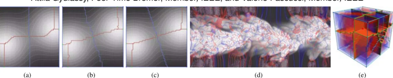
Fig. 1. Popular approaches for computing Morse-Smale complexes assign discrete gradient arrows in the direction of steepest descent, aligned with cells of the input mesh. Given a highly resolved sampling of two Gaussians, we show the results of the corresponding complex (a) which demonstrates severe artifacts in the positioning and direction of one-manifolds as can be seen from the level sets, which should be orthogonal. This paper introduces a randomized algorithm that better represents the gradient flow (b); and a deterministic variant that integrates probabilities to achieve near-optimal geometric reconstruction of the MS complex (c). We show the high-quality geometry, as well as the probability fields we compute for a two-dimensional jet (d); and a three-dimensional tetrahedrane molecule (e).

Abstract—Topological techniques have proven highly successful in analyzing and visualizing scientific data. As a result, significant efforts have been made to compute structures like the Morse-Smale complex as robustly and efficiently as possible. However, the resulting algorithms, while topologically consistent, often produce incorrect connectivity as well as poor geometry. These problems may compromise or even invalidate any subsequent analysis. Moreover, such techniques may fail to improve even when the resolution of the domain mesh is increased, thus producing potentially incorrect results even for highly resolved functions. To address these problems we introduce two new algorithms: (i) a randomized algorithm to compute the discrete gradient of a scalar field that converges under refinement; and (ii) a deterministic variant which directly computes accurate geometry and thus correct connectivity of the MS complex. The first algorithm converges in the sense that on average it produces the correct result and its standard deviation approaches zero with increasing mesh resolution. The second algorithm uses two ordered traversals of the function to integrate the probabilities of the first to extract correct (near optimal) geometry and connectivity. We present an extensive empirical study using both synthetic and real-world data and demonstrates the advantages of our algorithms in comparison with several popular approaches. Index Terms—Topology, topological methods, Morse-Smale complex.

1 INTRODUCTION

Since the development of the first combinatorial algorithms to com-pute the Morse-Smale (MS) complex from sampled data [1, 3, 9, 17] it has become widely used in a large variety of applications [5, 7, 15, 19, 22, 25]. Since then most of the algorithmic development has been focused on robust computation, topological consistency, and computa-tional efficiency. As a result there now exist comparatively simple, yet highly efficient, streaming and/or parallel algorithms to compute MS complexes from large data sets [13, 28–30]. These algorithms perform very well as long as one is interested in structural topological attributes of the data such as how many critical points exist [22] or average con-nectivity of 1-manifold networks [15]. More recently researchers have also begun to analyze the geometric information of topological fea-tures. For example Bennett et al. [2] compute length scales of local contours and Kasten et al. [19] find and track two dimensional vortex structures as unstable manifolds in the acceleration magnitude. How-ever, geometric fidelity so far has been mainly ignored when designing algorithms and, as shown in Fig. 1, all existing techniques tend to pro-duce poor geometry even for well-resolved functions. Furthermore, as discussed in more detail in Section 6, incorrect geometry often leads to incorrect connectivity thus casting doubts on subsequent analysis.

• Attila Gyulassy is with the SCI Institute, University of Utah, E-mail: [email protected].

• Peer-Timo Bremer is with Lawrence Livermore National Laboratory, E-mail: [email protected].

• Valerio Pascucci is with the SCI Institute, University of Utah, E-mail: [email protected].

Manuscript received 31 March 2012; accepted 1 August 2012; posted online 14 October 2012; mailed on 5 October 2012.

For information on obtaining reprints of this article, please send e-mail to: [email protected].

Even more problematic is the fact that traditional approaches will not converge with increasing mesh resolution to the correct solution.

In this context it is important to remember that there exists no MS complex for a sampled function since such functions are not “Morse-Smale.” Instead, all algorithms, discrete or otherwise, compute a quasi-MS complex as defined by Edelsbrunner et al. [9]. Intuitively, a quasi-MS complex is one that is consistent with the underlying theory, i.e., there exists a Morse function with this complex, yet not necessar-ily matching the flow behavior of the function sampled. In particular, Edelsbrunner et al. introduce a rarely used procedure call a Handle-Slide to correct the connectivity of a quasi-MS complex assuming the ability to perfectly compute the geometry of integral lines. By ignor-ing geometric fidelity most existignor-ing techniques may produce severely incorrect MS complexes making geometric quality a fundamental is-sue of correctness rather than only of visual improvement.

The geometry of the MS complex is defined by integrating gradient lines of the underlying flow which current discrete techniques con-struct through a local, greedy optimization. However, the locally op-timal choice may accumulate an arbitrarily large global error in the integration process and also make the algorithms highly dependent on local mesh orientation. Instead, we propose two new algorithms that both extract significantly better geometry than existing approaches and are guaranteed to converge to the correct geometry and connectivity under subdivision. The first algorithm uses the same algorithmic ker-nel as the best existing techniques but replaces the local optimization with a carefully designed random selection. It can easily be integrated into existing approaches, on average produces the correct complex, and its standard deviation from the mean converges to zero with in-creasing mesh size.

The second algorithm exploits the fact that typically only small por-tions of the gradient field matter to the geometry, namely those areas containing cell boundaries. By integrating the local probabilities of the first algorithm we construct a deterministic variant of the 1077-2626/12/$31.00 © 2012 IEEE Published by the IEEE Computer Society

rithm that extracts near optimal cell boundaries through a simple re-gion growing approach. Both algorithms are based on the common discrete framework and thus are combinatorial in nature, guaranteed to be topologically consistent, and applicable in any dimension. Our four main contributions are listed briefly below.

1. We introduce a randomized algorithm to compute MS complexes that significantly improves the geometric quality of the result when compared to existing techniques and converges with in-creasing mesh resolution. The algorithm is simple to implement, efficient, applicable in any dimension, and easily parallelized. 2. We introduce a second deterministic algorithm that directly

ex-tracts near optimal geometry without the need for refinement. 3. We provide an extensive empirical study comparing our

ap-proach with state of the art techniques using both synthetic and real-world data.

4. We provide a broad range of experiments demonstrating the su-perior quality and stability with respect to sampling density and mesh orientation.

2 RELATEDWORK

Despite the fact that the initial ideas were already discussed more than a century and a half ago [6, 26] the first practical algorithm to compute MS complexes of two dimensional, piecewise linear functions was in-troduced fairly recently [9]. In their seminal paper, Edelsbrunner et al. not only describe the first robust algorithm but also introduce the no-tion of a quasi-MS complex indicating a complex consistent with the theory yet not necessarily correct. Nevertheless, the algorithm relies on fairly complex data structures to maintain strict separation between one manifolds.

Bremer et al. [3] propose a simpler version of the same idea by demonstrating that by ordering the computations appropriately much of the algorithmic complexity can be avoided. They also introduce the first multi-resolution encoding of the complex. The algorithm pro-posed in [3] is interesting in so far it has been the only one capable of producing correct geometry for piecewise linear functions by lo-cally refining the input mesh. However, the 3D version of the same approach [8] has proven too complex to be practical and instead the focus has shifted to approaches based on discrete Morse theory, as discussed below.

Since the initial research, related concepts have seen rapid adop-tion in a wide variety of scientific applicaadop-tions. Laney et al. [22] use MS complexes to analyze Rayleigh-Taylor instabilities, Gyulassy et al. [15] to study the structure of porous media, Bremer et al. [4] to analyze turbulent combustion simulations, and Kasten et al. [19] to study vortical structures, to name just a few. In a related field, Koch et al. [21] used a probablistic method for tractography in diffusion tensor images. This work introduced a randomized approach, taking discrete, axis-aligned steps in tracing out probable diffusion paths, with proba-bilities weighted by alignment with the local tensor.

The most successful algorithms for computing Morse-Smale com-plexes for large, especially volumetric data rely on a discrete interpre-tation of Morse theory introduced by Forman [11]. In this framework, the key challenge is to compute a discrete gradient vector field from which the MS complex can then be extracted in a fairly straightfor-ward manner. Existing techniques share many characteristics yet each computes a discrete gradient vector field in a unique manner. At the core of every algorithm is the choice of discrete gradient vector that best represents the flow behavior of the underlying function and in this aspect all approaches are remarkably similar. Every approach as-signs weights to pairings based on the difference in function values of the cells to be paired. Here, we survey each technique highlighting the differences in order of computation and philosophy while pointing out the similarities of the results.

Lewiner [23] presented the first technique for constructing a dis-crete gradient field that agrees with the flow behavior of a scalar func-tion. In this approach, recently proved to be robust [24], the discrete gradient field is represented by a hyperforest. At each iteration of the GREEDY algorithm, the potential pair with maximum weight is se-lected and paired if it does not create a cycle. In this approach, the weight of a pairing is computed as the difference in function values at the barycenters of the two cells.

King et al. [20] introduced a technique to generate discrete Morse functions on simplicial complexes by modifying the Hasse diagram. The resulting diagram encodes both the discrete gradient arrows and the face relations needed to guarantee the construction of a discrete Morse function. At each step, the EXTRACTRAWalgorithm first cre-ates a directed edge in the diagram between a vertex and the edge in the direction of steepest descent, and then assigns pairs in the rest of the lower link. In effect, the “weight” of the initial vertex-edge pairing is given by the difference in function values of the two vertices inci-dent on the edge. An alternative, that scales this weight by one over the length of the edge, is also mentioned.

Gyulassy et al. [13] introduced an algorithm that assigns cells in order of increasing function value and increasing dimension, using the ordering to avoid acyclicity checks. In an extension to the algo-rithm [12], simply homotopy expansions are performed to avoid spuri-ous critical points. In this approach, the maximal weight pair is chosen for a cell, with weight being defined as the difference in value between the cell and the lowest vertex of its co-facet pair. This approach is used in [18] to design a blocked, parallel construction of MS complexes.

Reininghaus et al. [27,28] presented an approach for generating dis-crete vector fields at multiple scales by computing matchings of a cell graph using the Hungarian method. The mesh is represented using a Hasse diagram, where the weight of each edge is given by its align-ment to the gradient direction. Each iteration of the MORSEMATCH

-INGSEQUENCEalgorithm adds to the current matching the alternating path of heaviest weight. The unpaired cells of the maximum weight matching for any scalar function occur at critical points of the function. Although this technique finds a maximal global weight, the global sum is composed of aggregating local weights, therefore, in effect, gradient pairs are assigned in the steepest direction.

Robins et al. [29] present a technique that computes the discrete gradient on the lower star of a vertex. The PROCESSLOWERSTARS

algorithm pairs each vertex with the edge in its lower star that touches the lowest vertex in the lower link. Subsequently, remaining cells in the lower star are paired using simple homotopy expansions, when possible, or assigning critical cells. Effectively, this approach maxi-mizes the weight of a vertex-edge pairing, the weight being the differ-ence in function values of the two vertices incident on the edge. The independent assignment of gradient arrows in this approach allows an embarrassingly parallel implementation.

Shivashankar et al. [30] also present an embarrassingly parallel technique for computing the gradient. First, a discrete Morse func-tion is computed in which every cell is critical. However, the funcfunc-tion is defined such that the ASSIGNGRADIENT algorithm simply looks for the co-facet with lowest value to pair a cell. The recursively de-fined function ensures that a vertex will always be paired with the edge whose other endpoint has lowest value,i.e., in the direction of steepest descent.

In summary, while all approaches use slightly different techniques they all assign arrows based on steepest-descent and thus produce very similar geometry. For example, two functions for which all tech-niques [13,20,23,27–30] produce identical discrete gradient fieldsare (1) distance from a point,f(x) =c||x−p||, and (2) any constant slope, f(x) =cx+b. The differences for more complex functions are min-imal, and each technique follows the same pattern of greedy assign-ment. In the examples in this paper, we use the algorithm of Gyulassy et al. [13] as a representative of this class of approaches.

3 BACKGROUND

Scalar valued volumetric data is most often available as discrete sam-ples at the vertices of an underlying mesh. Morse theory has been well-studied in the context of smooth scalar functions, and has been adapted to such discrete domains. We first present some basic definitions from smooth Morse theory, and then present the discrete analogue. 3.1 Morse Functions and the MS Complex

Letfbe a real-valued smooth mapf:M→Rdefined over a compact

d-manifoldM. A pointp∈Mis critical when|∇f(p)|=0,i.e. the gradient is zero, and is non-degenerate when its Hessian (matrix of second partial derivatives) is non-singular. The functionf is aMorse functionif all its critical points are non-degenerate and no two critical points have the same function value. In this case theMorse Lemma

states that there exists local coordinates aroundpsuch that fhas the followingstandard form: fp=±x2₁±x2₂· · ·±x2_d. The number of minus signs in this equation gives theindex of critical point p. In three-dimensional functions, minima are index-0, 1-saddles are index-1, 2-saddles are index-2, and maxima are index-3.

An integral line in f is a path inMwhose tangent vector agrees with the gradient of f at each point along the path. The integral line passing through a pointpis the solution to ∂

∂tL(t) =∇f(L(t)),∀t∈R, with initial valueL(0) =p. Each integral line has an origin and des-tination at critical points of f. Ascendinganddescendingmanifolds are obtained as clusters of integral lines having common origin and destination respectively. The descending manifolds of f form a cell complex that partitionsM; this partition is called theMorsecomplex.

Similarly, the ascending manifolds also partitionMin a cell complex.

A Morse function f is aMorse-Smale functionif ascending and de-scending manifolds of its critical points only intersect transversally. An index-icritical point has ani-dimensional descending manifold and a(d−i)-dimensional ascending manifold.

3.2 Discrete Morse Theory

Discrete Morse theory is at the heart of current techniques for ef-ficiently computing Morse-Smale complexes. We provide a brief overview with basic definitions from Forman [11], and we refer the reader to this introductory work for an intuitive description. A d-cell is a topological space that is homeomorphic to a Euclideand-ball Bd={x∈Ed:|x| ≤1}. For cellsα andβ,α<β means thatαis a faceofβ andβ is aco-faceofα,i.e., the vertices ofα are a proper subset of the vertices ofβ. Ifdim(α) =dim(β)−1, we sayαis afacet ofβ, andβis aco-facetofα, and denote thisα<˙β. When necessary to clarify the discussion, we may denote the dimension of ad-cellα withα(d). Thestarof a cellα, denotedSt(α), is the set of co-faces ofα. Thelower starofα, denotedSt−(α)is subset ofSt(α)where each element has lower function value. Thelinkofαis the closure of the star, minus the star itself,Lk(α) =St(α)−St(α). Similarly, the lower linkofαisLk−(α) =St−(α)−St−(α)

LetKbe a regular complex that is a mesh representation ofM. The

barycenter B:K→Mof ad-cellα∈K,B(α), is the average of its vertices. A functionF:K→Rthat assigns scalar values to every cell

ofKis adiscrete Morse functionif for everyα(d)∈K, its number of co-facets|{β(d+1)>˙α|F(β)≤F(α)}| ≤1, and its number of facets

|{γ(d−1)<˙α|F(γ)≥F(α)}| ≤1. A cellα(d)is critical if its number of co-facets|{β(d+1)>˙α|F(β)≤F(α)}|=0 and its number of facets

|{γ(d−1)<˙α|F(γ)≥F(α)}|=0, and has index equald.

Avectorin the discrete sense is a pairing of cellshα(d),β(d+1)i, where α<˙β. We say that an arrow points from α(d) to β(d+1). The direction of the arrow relates the combinatorial notion of the pairing to the geometric interpretation of the flow, and is given by B(β(d+1))−B(α(d)). Intuitively, this vector simulates a direction of flow. A discrete vector field V on K is a collection of pairs hα_i(d),β_i(d+1)iof cells ofKsuch that each cell is in at most one pair ofV. A critical cell is unpaired. Given a discrete vector fieldV onK, aV -pathis a sequence of cells

α₀(d),β₀(d+1),α₁(d),β₁(d+1),α₂(d), . . . ,βr(d+1),α_r(₊₁d)

such that for eachi= 0,..., r, the pairhα_i(d),β_i(d+1)i ∈V, andα_i(d)and α_i(₊₁d) are both facets ofβ_i(d+1). AV-path is the discrete equivalent of a streamline in a smooth vector field. A discrete vector field in which allV-paths are monotonic inF and do not contain any loops is adiscrete gradient field, denotedG, of a discrete Morse function. When constructing a discrete gradient field, we say that Gisvalid if these two conditions are met. The discrete equivalent offlowin a continuous gradient is taking astepin a V-path,i.e., we say thatα_i(₊₁d) is one step fromα_i(d). The critical cellα_r(₊₁d) at the end of a V-path is thedestinationof the V-path. We also sayα_r(₊₁d) terminatesthe V-path.

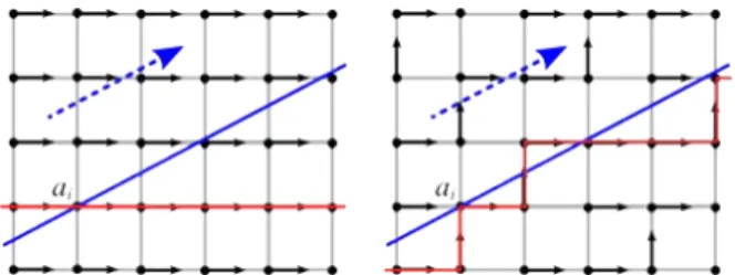
Fig. 2. For a function with a constant negative gradient (blue arrow), approaches using the locally steepest descent produce identical pair-ings at all vertices (left). The error of the V-path (red) from the integral line (blue) passing through a vertexai accumulates with each step. In our randomized approach, a vertex can be paired with any vertical edge with some probability, producing a V-path with lower overall error (right). 3.3 Generic kernel for computing discrete gradient fields The algorithms surveyed in Section 2, while quite varied in their spe-cific approaches, roughly implement the same underlying functional-ity. The algorithmic kernel proceeds in the following four steps:

1. Pick a yet unassigned cell

2. Find its potential pairings and assign weights 3. Check for the validity of the pairing

4. Assign gradient arrow of highest weight or declare a critical cell Each algorithm may perform these steps in unique ways. For exam-ple, Lewiner [23] picks the cell whose potential pairing has the highest weight, and uses a search structure on a graph representation of the gradient to check that the pairing not create a cycle. In contrast, Shiv-ashankar et al. [30] first define a discrete Morse function for which the order in which cells are picked is irrelevant. Each cell has one unique possible pair derived directly from the function, and the validity of the pairing is guaranteed by the definition of the function. Gyulassy et al. [13] picks cells in order of increasing function value and dimension to guarantee that any pairing is valid. Robins et al. [29] selects any unassigned vertex, pairs it with the edge in the steepest downwards di-rection, and assigns the rest of the cells in the lower star of the vertex. Acyclicity is guaranteed by simulation of simplicity used in generating the lower link.

4 RANDOMIZEDGRADIENTFIELDS

One of the most significant drawbacks of existing techniques is their poor geometric approximation of gradients which leads to incorrect connectivity. Due to their local, greedy assignment of gradient arrows they may produce arbitrary large errors even in regions of constant gra-dients. Consider the example shown in Fig. 2: The (inverse) gradient of a function is indicated by the blue arrow and assumed to be con-stant for all cells. Current techniques will, at each vertex, determine the locally best pairing, causing all gradient arrows to be chosen hori-zontally. Thus, the discrete V-path passing through a vertexαi(shown in red) will diverge drastically from the integral lineLin f. The fun-damental problem is that while each arrow is chosen to minimize the local error, all arrows deviate in the same direction from−∇f and collectively cause major artifacts.

We propose a randomized approach that on average will produce significantly better results. Instead of choosing the locally optimal gra-dient arrow atα, we pick among all potential valid pairs with a certain probability designed such that the expected V-path will approximate the integral line.

4.1 Algorithm

To construct a randomized gradient field we use the standard discrete kernel discussed in Section 3.3 with a modified pairing. Similar to ex-isting techniques, given an unassigned cellα we compute for each of its co-facetsβia weight for the potential pairhα,βii. However, instead of picking the pair with maximal weight, we instead chooseat random from the potential pairs, with probabilities assigned proportional to the weights. We pair each vertex with an edge probabilistically using these weights, and use the simple homotopy expansion described by Robins et al. [29] to complete the pairings for all other cells in the lower star of the vertex.

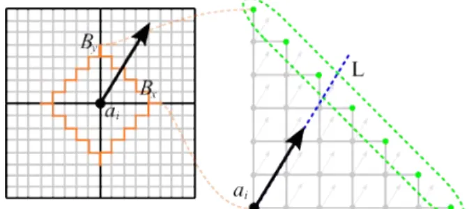
Fig. 3. On the left, the original grid (black) is uniformly subdivided (gray lines) until the a neighborhood (orange outline) aroundαican be mod-eled using a piecewise constant gradient. The right shows the lower right quadrant ofN, the cells that have a non-zero probability of being in a V-path passing throughαi. The green dots denote the potential exit point ofPα_{fromN, while the blue dot denotes the exit point ofI}α_from N.

More specifically, letαbe a 0-cell, and−∇f(B(α))be the negative gradient offatB(α)the barycenterα. The weight of a potential pair hα,βiiis defined as the dot-product between the geometric realization of the pairB(βi)−B(α)and the negative gradient−∇f(B(α)). Fur-thermore, all negative weights - indicating invalid pairs - are clamped to zero:

w(hα,βii) =max{(B(α)−B(βi))·(−∇f(B(α)),0} (1) Using these weights, the probability of pickinghα,βiiis defined as

Pr(hα,βii) =w(hα,βii)/

_∑

w(hα,βji). (2)

Note, that the probabilities are invariant under uniform scaling of both the mesh as well as the gradient magnitudes.

4.2 Geometric Convergence

One of the advantages of our approach is that under subdivision, V-paths in the resulting gradient field will converge to integral lines in f. We say a V-path containingαconverges to the integral line passing throughB(α)when the Hausdorff distance between the V-path and in-tegral line goes to zero. It is well known that with increasing mesh resolution a piecewise constant approximation of a gradient field will converge to the continuous gradient. In this section we will show that V-paths of the randomized field will converge to integral lines in a given piecewise constant gradient field and thus ultimately to any gra-dient field. In contrast, existing approaches do not faithfully reproduce even constant gradients, and thus will produce incorrect results even for well resolved functions.

For simplicity letγ= [0,1]2be the unit square with a constant gra-dient∇f= (−fx,−fy)and wlg. assumefy>fx>0. Then the integral line passing through the origin is the lineL:y= fy/fxx. Here we will show that ifγis subdivided into a regularn×ngrid with gradient arrows assigned as discussed above then afternsteps the expected de-viation fromLis 0 with a standard deviation that behaves like 1/√n.

Given the assumptions above, when pairing a vertex, only potential pairs in positivexor positiveydirection inγhave non-zero weights. All potential pairs in the positivexdirection inγwill have a weight of w(hα,βxi) = (1,0)·(fx,fy) =fxand all potential pairs in the positive ydirection have weightw(hα,βyi) =fy. Therefore, the probability of pairing a vertex with its horizontal edgeβxis:

Pr(hα,βxi) = fx fx+fy

= fx+fy−fy

fx+fy

=1−Pr(hα,βyi). Consider assigning gradient arrows starting at the origin one pair at a time. Each assignment extends the V-path containing the origin by one pair. Each time we step to the right with probabilityPr(hα,βxi)

and step upwards with probabilityPr(hα,βyi). The number of hor-izontal steps inntrials follows a binomial distribution with parame-tersnandPr(hα,βxi). Therefore, the expected number of horizontal steps afterntrials isnPr(hα,βxi)and the expected number of

ver-tical steps isn−nPr(hα,βxi). Normalizing by the grid size, it fol-lows that the expected endpoint of the V-path starting at the origin is Pr(hα,βxi),Pr(hα,βyi)

, right onL. Furthermore, the standard deviation of the binomial distribution normalized by the grid size is Pr(hα,βxi)Pr(hα,βyi)/√n.

The same argument holds for unit cubes of higher dimen-sions using multinomial distributions. Let the probabilities of pairing an edge in the direction xi be Pr(hα,βxii) then

the expected endpoint of the V-path after n steps will be

(Pr(hα,βx₀i),...,Pr(hα,βxdi))with the standard deviation in

dimen-sionigiven by(Pr(hα,βxii)(1−Pr(hα,βxii)))/

√

n. This proves that with increasing grid resolution, V-paths of a randomized gradient field will converge to integral lines of a given piecewise constant gradient with standard deviation approaching zero. Given that any gradient field can be approximated up to an arbitrarily small error by a piece-wise constant field, V-paths in a randomized gradient field will con-verge to integral lines of the continuous gradient under subdivision. 4.3 Randomized Gradient Fields of Sampled Functions In practice, we are primarily dealing with sampled functions in which case we must estimate the gradient vector at vertices. There exist two options: First, one can use any of the standard gradient estimation techniques to compute a gradient per vertex and apply the algorithm as described above. Second, one may compute a modified version of the weight that admits gradient discontinuities on the boundary of cells. When using a per-vertex gradient computed with a gradient estimation technique, such as central differences, it is possible that the gradient arrow point in a direction that is locally “uphill”, e.g. in a direction of increasing function value. To avoid potential cycles the weight of each potential pair in the lower star will be set to zero, and the vertex will be marked critical.

For simplicity and/or in a parallel environment it may be conve-nient to compute a gradient per highest dimensional cell (i.e. quads in 2D, voxels in 3D). In this case all lower dimensional cells have mul-tiple gradient vectors assigned to them. In this case Equation 1 must be changed to use the appropriate gradient for eachβi. Note that for regular grids the dot product of, for example, an edge in a two dimen-sional mesh with its two gradients on either side will naturally produce consistent values. In fact, since the probabilities are scale independent one can assume a regular grid with edges of length one in which case weights can be computed as the difference in function values at their endpoints.

5 A DETERMINISTICAPPROACH FORACCURATEGEOMETRY The algorithm discussed above will construct a gradient field that on average is correct and will converge with increasing sampling rates to the gradient of f. However, in practice subdivision is typically infea-sible for larger data sets. Therefore, the true value of the randomized gradient field is that it is expected to produce a good approximation of f’s gradient even though the quality of any individual V-path cannot be guaranteed. This lack of guarantees is inconvenient especially for large data sets where the computation cannot be easily repeated but geometric quality is important.

In this section we present an extension of randomize gradient fields that leads to a deterministic algorithm guaranteed to extract high qual-ity geometry. The algorithm is based on the insight that the geometry of the MS complex depends only on a small fraction of V-paths, those on the boundaries between ascending and descending manifolds. In particular, one may rephrase the problem of constructing a high qual-ity MS complex as constructing a discrete gradient in which arrows do not cross a-/descending manifold boundaries. To this end we integrate the probabilities defined in Section 4 in order of increasing function value to compute for each cell the probability of its V-path ending at a particular critical cell. We then assign gradient arrows to minimize the number of arrows crossing manifold boundaries. Assigning all gradi-ent arrows of, for example, a two dimensional grid according to their minima distribution leaves exactly those cells unassigned that form the boundary of the ascending manifolds. These cells are filled in by as-signing cells according to their saddle distributions. In a second pass we then construct the distributions according to maxima to compute the boundaries between descending manifolds but restrict the compu-tation to be consistent with the first pass.

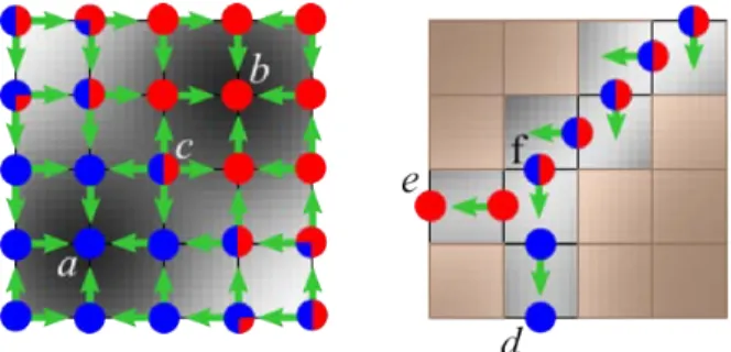
Fig. 4. This figure represents member distributions of cells as a pie-charts,i.e., the area of a particular color indicates the probability that the cell will flow to the critical point represented by the color. On the left, there are two minima,aandb, colored blue, and red, respectively. The green arrows indicate the discrete gradient arrows that have non-zero probability of being picked in a randomized approach. At vertexc, all four directions have equal probability of being paired and therefore, the member distributions of the vertices at the other end of each arrow are averaged to getµc. The image on the right illustrates a scenario where a V-path splits. In this case,µf represents this split by assigning equal probability toeandd. The shaded area indicates cells that have zero probability of belonging to any V-path terminating at a critical 1-cell. 5.1 Computing Membership Distributions

We represent the probabilities of a (randomized) V-path ending at cer-tain critical cells as amembership distributionµα:K→Rwhich for

eachd-cellαand all cellsκ∈Kdefines the probability of the V-path containingαto end atκ. Membership distributions are defined recur-sively starting at critical cells. In the following, letβ be a co-facet of α, andLk−_β(α)denote the set ofd-cells in the lower link ofαthat are also facets ofβ. LetPrdenote the selection probability function from Equation 2 in Section 4.1. Then:

µα(κ) =            0 ifdim(α)6=dim(κ) 1 ifαis critical andκ=α 0 ifαis critical andκ6=α

∑

_∑

The first case reflects the fact thatµαwill only be used to assign

ar-rows betweend-cells and(d+1)-cells and thus we are only concerned with the index-dcritical cells that can be reached fromα. In the sec-ond case,α itself is critical, therefore it has probability one since all possible V-paths containingαmust terminate there. Consequently, in the third case, ifαis critical the probability of reaching any other cell is zero. The final case defines the membership distribution of a cell recursively as the weighted combination of the membership distribu-tions of cells in its lower link. Intuitively, the probabilities indicate the likelihood that a V-path containinghα,βiexists which when multi-plied with the probability that a V-path containingρ (β’s other facet) ends atκdefines the probability that a path containingαreachesκvia

hα,βi. Summing over allβ’s, thus, computes the probability that any V-path containingαterminates atκ.

Since the membership distribution of any cell depends only on membership distributions of cells with lower function value, these dis-tributions can be computed efficiently by processing cells in order of increasing value.

5.2 Gradient Computation

The general framework we use for assigning discrete gradient arrows borrows heavily from published techniques [12–14, 23, 29]. For exam-ple, we extend a function sampled at vertices to values at every cell to assigning a cell the value of its highest vertex. We use the region-growing approach introduced by Gyulassy et al. [13] to assign discrete gradient arrows on the interior of an ascending manifold. We then per-form simple homotopy expansions [12, 29]. Indeed, as with every pre-vious technique, we pair a discrete gradient arrow in the direction that maximizes the weight of the pairing. However, the new weight func-tion derived below assumes a particular order of assignment, which

requires subtle variations of existing approaches.

In our algorithm, we first compute thed-cell to(d+1)cell arrows on the interior of an ascending(D−d)-manifold, whereDdenotes the maximum dimension of a cell in the meshK. We then assign all possible discrete gradient arrows that preserve the simple homotopy type of the ascending manifolds. For volumetric data, we first assign all cells in the interior of ascending three-manifolds, then ascending two-manifolds, etc. until all cells are assigned. Fig. 5 illustrates these steps for a simple two-dimensional example. Below we report pseudo-code for the corresponding algorithm.

In the following, letKbe the underlying mesh,Fa function map-ping a cell to a scalar value, andGthe discrete gradient field. The gradient field is defined as a set of pairs of cells, where each pair repre-sents an arrow pointing from the lower to the higher dimensional cell. We pair a cell with itself to denote criticality. We call cellsassignedif they can be found inG.

1: ComputeGradient(K, F) : 2: G ={} 3: ford∈[0,D]do 4: G = AssignArrows(d, K, F, G) 5: G = HomotopyExpand(K, F, G) 6: end for 7: return G

The functions AssignArrows() and HomotopyExpand() simply add new pairs to the discrete gradient field G.

Weight of a Pairing. In the process of computing the discrete gra-dient field, our technique assigns a weight to a potential pairhα,βii based on (1) the known destinations (critical cells) of V-paths assigned so far in G, and (2) the membership distributionµα of the lower

di-mensional cell. Letα be an unassignedd-cell, andCbe the set of

(d+1)-cells it can be paired with. Formally,Cis the set of unassigned cells in the lower star ofα that are its co-facets,i.e.,C={St−(αi)| β>˙α,β ∈/G}. We callC candidates, since pairingα with any cell inCproduces a valid gradient field. For each βi∈C, we assign a weight to the potential pairhα,βiito minimize the number of arrows crossing manifold boundaries. When pairingα, each cell in the lower linkγi∈Lk−(α)has already been paired. In fact,γiis part of V-paths that do not change belowγiwith any subsequent gradient arrow assign-ments, and we can find their terminating critical cells. It is well-known that in dimensions higher than one, V-paths can split, for example, as illustrated in Fig. 4 (right). Therefore, letDγibe the set of critical cells

that terminate V-paths flowing throughγi. The weight ofhα,βiiis defined as: w(hα,βii) =

_∑

∑

Intuitively, this weight represents the likelihood that α belongs to the same ascending manifolds as the facets ofβ. Therefore, higher weights indicate potential pairs that are less likely to cross boundaries of ascending manifolds. Just as the definition of the distributions, the weight depends on the fact that everyd-cell in the sub-level complex of F(α) has been assigned. Therefore every cell in the lower link of α belongs to assigned V-paths terminating at critical cells in G. Pro-cessing cells in order of increasing function value as described below guarantees this property.

Assigning Gradient Arrows. The following algorithm computes the d-cell to(d+1)-cell gradient arrows on the interior of an ascending

(D−d)-manifold. The unassignedd-cells inKare processed in order of increasing function value, with ties broken by simulation of simplic-ity [10]. By processing cells in sorted order, in effect, we are growing the spanning trees ofd-cells of the sub-level complex ofK. As each d-cell is visited by the algorithm, its potential pairs, the candidatesCare identified. If there are no candidates for pairing, thed-cell is assigned critical. Otherwise, the one maximizing the weight function given in Equation 3 is chosen. The algorithm terminates when alld-cells are assigned.

1: AssignArrows(d, K, F, G) :

2: Kd={αd∈K|dimension ofαisd}

Fig. 5. A discrete gradient field of a sampled function indicated in gray is computed using the algorithms of Section 5. From left to right: First, we pair vertices and edges according to the maximal weight, then pair edges and faces in a simple homotopy expansion. Second, we pair the remaining edges and cells according to their weight and faces and voxels (not shown) in the corresponding homotopy expansion. Finally, we pair faces and voxels by weight and mark all remaining unpaired voxels as critical.

4: forαi∈Kddo 5: C ={β∈St−(αi)|β>˙α} 6: if C=/0 then 7: G=G∪ hαi,αii 8: else 9: βj=argmax_βi∈C(w(hα,βii)) 10: G=G∪ hαi,βji 11: end if 12: end for 13: return G

The function argmax() simply returns the argument that maximizes its value,i.e., the(d+1)-cell where the pair{α,βi}has highest weight. Simple Homotopy Expansion LetKn⊆K be the subcomplex of assigned cells ofK after selectingnpairs. Assigning a gradient ar-row adds exactly two cells to this subcomplex. An assignment of a gradient arrow is asimple homotopy expansionif Kn is homotopic toKn+1. In practice, ad-cell to (d+1)-cell arrow can be inserted without changing the homotopy type of the subcomplex when (1) all faces of the d cell are assigned, and (2) thed-cell is the only unassigned face of the(d+1)-cell. The only time we prohibit this expansion is when the arrow would point “uphill”, i.e., the value of the d+1 cell is strictly larger than the value of the d cell in F. 1: HomotopyExpand(d, K, F, G) : 2: H={α∈K|# unassigned facets inGis 1} 3: whileH6=/0do 4: α= PopFirst(H) 5: β= unassigned facet ofα 6: if F(α)≤F(β) then 7: G=G∪ hα,βi 8: update(H) 9: end if 10: end while 11: return G

When a gradient arrowhα,βiis assigned, the number of unassigned facets of all co-facets ofαandβ decreases, and update() inserts the co-facets having exactly one unassigned facet intoH.

5.3 A Two-Pass Approach

The algorithm described above only takes the geometric accuracy of ascending manifolds into account. To get both accurate ascending and descending manifolds, we use the result of the first pass to restrict a second pass. In the second pass, we repeat the algorithm on the com-plement ofKusing the negative ofFwith one change: We only con-sider candidates for pairing cells belonging to the interior of the same dimensional ascending manifold. Figure 6 illustrates this approach. 6 RESULTS

In this section we present experiments comparing the geometric qual-ity of the MS complex computed using previous steepest-descent tech-niques, the new randomized approach, and the two-pass, deterministic variant. We compute and visualize the MS complex from a discrete gradient field using the techniques described by Gyulassy et al. [16]. For clarity we begin with simple two-dimensional examples. Fig. 7

Fig. 6. A first pass computes accurate geometry for the ascending man-ifolds (left). In the second pass (right), arrows in ascending 1-manman-ifolds (pink lines) may only be paired with one another. In each image, the hazy cells indicate the maximum probability of a cell belonging to a par-ticular manifold - the darker the color, the lower the probability. The boundaries between cells in our MS complex naturally occur where probability of membership is lowest.

(a) (b) (c)

(d) (e) (f)

(g) (h) (i)

Fig. 7. The top row, (a-c) show the function from Fig. 1, up-sampled four times in each direction. Note that the steepest-descent construc-tion in (a) does not improve with increased mesh resoluconstruc-tion. We show five realizations of our randomized approach (b), and our near-optimal approach (c). In (d-f) we show the same techniques applied to f(x,y) =arctan(−y/|x|)forr1<||(x,y)||<r2. In these examples, the

smooth integral line starting at the saddle forms a circle. The same function is used sampled four times finer in each direction in (g-i).

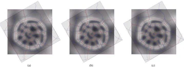
(a) (b) (c)

Fig. 8. These images illustrate the dependence of the steepest-descent construction (a) on the mesh orientation, and the resilience of the two proposed techniques (b, c). The same underlying function is re-sampled onto one grid oriented vertically, and another grid rotated 30 degrees from vertical. We overlay the complexes computed for each, aligning them with the orientation of the underlying function. Excluding boundary artifacts, the complexes of the locally maximizing approach (a) vary significantly, the randomized approach (b) displays better behavior, and the complexes of our two-pass approach (c) vary only by the width of a cell.

(a) (b) (c) (d) (e) (f)

Fig. 9. In (a-c), minima along two “valleys” and maxima along a “ridge” are separated by saddles. While the complex generated by the steepest descent approach (a) isconsistent, it connects the saddles and extrema poorly. Our randomized approach performs better (b), and the two-pass approach (c) produces a very accurate solution. In (d-f) we show the resilience of our techniques to flat regions in the data. (d) The region growing variant of the steepest-descent algorithm described by Gyulassy et al. [12] provides a reasonable approximation to ascending 1-manifolds (pink lines), However, the descending lines simply follow the steepest-descent direction given by simulation of simplicity [10]. We apply the same order of assignment, but with our randomized kernel (b), resulting in a more intuitive traversal of flat regions. In the two-pass approach, distance (in the number of steps in a V-path) naturally factors into the weight function, steering the geometry of the complex perpendicularly away from the boundary of a flat region.

and 1 show how each algorithm responds when the mesh is subdi-vided. We sample two smooth functions on a regular grid: The first is the sum of two Gaussians; The second is a function with semi-circular integral lines. In both cases existing approaches create severe artifacts in both direction and shape of the one-manifolds. Moreover, the ar-tifacts are unaffected by the increase in resolution. The randomized algorithm, while producing somewhat wavy patterns, already signif-icantly improves the geometry and converges to the correct solution with increasing mesh resolution. The two pass approach extracts the correct geometry up to the resolution of the mesh, and a higher reso-lution mesh unsurprisingly allows more accurate geometry.

Fig. 8 shows the resilience of each algorithm to changes in the ori-entation of the underlying mesh. Here, an underlying function is sam-pled by two grids, rotated 30 degrees from one another. The com-puted complexes are overlaid, for each technique, for visual compar-ison. Again the steepest-descent assignment shows large variations and artifacts, while the randomized approach shows a good correspon-dence, and the two-pass algorithm extracts identical geometry to the extent possible.

Fig. 9(a-c) compares the topological correctness of each technique. In this case, we connect saddles along a perturbed valley to maxima on a perturbed ridge, and saddles from the ridge to the minima. In this case we consider the topological information encoded by an arc of the MS complex to becorrectwhen the critical points at the ends are connected by an integral line in the underlying function. An infinites-imal perturbation of the function can redirect integral lines, therefore any MS complex that isconsistentis a valid output (a quasi-MS com-plex in the sense of [9]). However, the output ideally should be both

consistent and correct for some smooth interpretation of the sampled function. In this sense, our randomized and two-pass techniques pro-duce a far more correct complex.

Imaged data is often captured with limited precision or quantized to reduce its size. This often leads to degenerate regions with zero gradients everywhere. Therefore, the behavior of algorithms in such “flat” regions is of significant interest. In Fig. 9(d-f) we compare the results of our new algorithms against the best know previous tech-nique of Gyulassy et al. [14], where gradient arrows are assigned in a breadth-first order to route V-paths efficiently across flat regions.

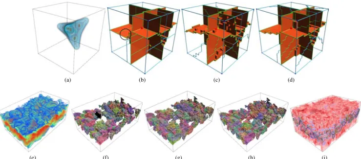
Finally, Fig. 10 compares our algorithms against steepest-descent techniques for two volumetric data sets. As before, the steepest-descent algorithm produces significant artifacts as exemplified by the shape of the one-manifolds for the tetrahedrane. Note that in the jet example, the mangled geometry causes entire Morse crystals to disap-pear leading to significant changes in the structure of the complex.

Results were generated on a commodity laptop, with 4Gb main memory and 2.2GHz Intel processor. Our algorithms were imple-mented in C++. The running time and total memory used for each example is summarized in table 1. The table shows results for both a serial implementation of the randomized approach, as well as the deterministic algoirthm for computing accurate geometry. Storing the membership distributions was responsible for the large memory foot-print of the latter approach.

7 DISCUSSION

Our results highlight the difficult cases for a local steepest-descent al-gorithm. In many cases, such an algorithm produces acceptable

re-(a) (b) (c) (d)

(e) (f) (g) (h) (i)

Fig. 10. We show results for two three dimensional datasets. The top row shows the ascending 2-manifolds, arcs, and nodes of the electron probability density function of a tetrahedrane(C4H4) molecule (a). (b) Uses the steepest-descent, (c) the randomized, and (d) the two-pass approach. Note the shape of the arcs, and the gradual decline of the surface of (d) with respect to (b)(circled). Figure 1(e) shows the integrated probability functions for this dataset. The bottom row (e-i) displays thedissipation elementsin a cross-flow jet flame. Each element is defined by the boundary of an ascending 3-manifold on the interior of the flame, and the same filters are used to select from each complex computed using steepest-descent (f), randomized (g), and two-pass (h) gradient fields. Several of the ascending 3-manifolds in the complex computed using steepest-descent (f) are missing (arrow), possibly due to handle slides. (i) shows the integrated probabilities for our two-pass approach, with blue indicating low ascending manifold membership probability, and red indicating low descending manifold membership probability.

Table 1. Run time and maximum memory usage to construct the discrete gradient field using the randomized approach(section 4) and the deterministic one(section 5). The times reported for the randomized approach are for a single thread.

Randomized Deterministic XxY(xZ) # Vert Time(s) Memory(Mb) Time(s) Memory(Mb)

gauss60 60x60 3600 0.047 <1 0.124 2 gauss240 240x240 57,600 0.546 4 2.044 12 JetSlice 768x512 393,216 4.509 14 16.54 49 C4H4 24x24x24 13,824 0.374 5 5.7 18 Fuel 64x64x64 262,144 4.509 12 14.64 40 JetChi 192x84x128 2,064,384 57.02 100 256.3 411

sults. In particular, sharp features, such as sharp ridge and valley lines are typically well-represented by a steepest-descent algorithm. In these cases, our approaches perform just as well, since there tends to be little variation in the probable membership of a cell.

In practice, we represent membership distributions as a sparse map, and compute them during the region-growing construction. In this case, only the membership distributions on the growing front of our region need to be available. When everyd-dimensional neighbor of ad-cell has been assigned, its membership distribution can safely be discarded. In our implementation, the memory requirements of mem-bership distributions is given by a constant times the number of cells crossed by the largest isosurface. The constant is bounded by the max-imum number of criticald-cellsαcould flow to. In equation 3, the set Dγ of criticald-cells that terminate the assigned V-paths containing

a cell is also computed incrementally. When a gradient arrow is as-signed into a pairhα,βi,Dαit is simply the union ofDγ forγ<˙β. In

practice, the running time of our algorithm isC2∗nlogn.

The one case our two-pass algorithm does not handle correctly is the interior of a topologicalstrangulation. The geometric accuracy of our approach depends on finding the boundary between distinct re-gions - in a strangulation, an a-/descending manifold borders itself. In this case, when each potential pairing has equal weight, we resort to steepest-descent.

8 CONCLUSION ANDFUTUREDIRECTIONS

We have presented two new approaches for computing discrete gradi-ent fields that better approximate the gradigradi-ent flow a scalar function.

Our first technique is simple and can be plugged in as-is to parallel computation of the MS complex. Our second technique provides ac-curate geometry, but at the cost of serial computation. As the MS com-plex is becoming more widely used in analysis, geometric guarantees become necessary. We will investigate techniques for providing nu-merical error estimates for analysis performed using the MS complex. The most significant current limitation is the heavier memory footprint of the two-pass approach. Although the two-pass algorithm computa-tion is serial, there are several potential avenues for its parallelizacomputa-tion. We are investigating a GPU implementation of the membership distri-bution computation, maintaining efficiency by only keeping the most probable elements ofµ. We plan on addressing the memory limita-tion initially through a divide-and-conquer approach on a distributed memory system. Alternatively, the complex could be computed in parallel using any previous technique, with a multi-threaded approach applying the two-pass algorithm to “fix” the gradient on independent sub-regions delimited by the boundaries of existing ascending and de-scending manifolds.

ACKNOWLEDGMENTS

This work is supported in part by NSF OCI-0906379, NSF OCI-0904631, DOE/NEUP 120341, DOE/MAPD DESC000192, DOE/LLNL B597476, DOE/Codesign P01180734, and DOE/SciDAC DESC0007446.

REFERENCES

[1] E. Babson and P. Hersh. Discrete Morse functions from lexicographic orders.Transactions of the American Mathematical Society, 3(457):509– 534, 2005.

[2] J. Bennett, V. Krishnamurthy, S. Liu, V. Pascucci, R. Grout, J. Chen, and P.-T. Bremer. Feature-based statistical analysis of combustion sim-ulation data. IEEE Transactions Visualization and Computer Graphics, 17(12):1822–1831, 2011.

[3] P.-T. Bremer, H. Edelsbrunner, B. Hamann, and V. Pascucci. A topolog-ical hierarchy for functions on triangulated surfaces.IEEE Transactions on Visualization and Computer Graphics, 10(4):385–396, 2004. [4] P.-T. Bremer, G. Weber, V. Pascucci, M. Day, and J. Bell. Analyzing

and tracking burning structures in lean premixed hydrogen flames.IEEE Transactions on Visualization and Computer Graphics, 16(2):248–260, 2010.

[5] P.-T. Bremer, G. Weber, J. Tierny, V. Pascucci, M. Day, and J. B. Bell. Interactive exploration and analysis of large scale simulations using topology-based data segmentation. IEEE Transactions on Visualization and Computer Graphics, 17(99), 2010.

[6] A. Cayley. On contour and slope lines. The London, Edinburgh and Dublin Philosophical Magazine and Journal of Science, XVIII:264–268, 1859.

[7] F. Cazals, F. Chazal, and T. Lewiner. Molecular shape analysis based upon the morse-smale complex and the connolly function. In Proceed-ings of the 19th Symposium on Computational Geometry, SCG ’03, pages 351–360, New York, NY, USA, 2003. ACM.

[8] H. Edelsbrunner, J. Harer, V. Natarajan, and V. Pascucci. Morse-Smale complexes for piecewise linear 3-manifolds. InProceedings of the 19th Symposium on Computational Geometry, pages 361–370, 2003. [9] H. Edelsbrunner, J. Harer, and A. Zomorodian. Hierarchical

Morse-Smale complexes for piecewise linear 2-manifolds. Discrete Computa-tional Geometry, 30:87–107, 2003.

[10] H. Edelsbrunner and E. P. M¨ucke. Simulation of simplicity: A technique to cope with degenerate cases in geometric algorithms. ACM Transac-tions on Graphics (TOG), 9:66–104, 1990.

[11] R. Forman. A user’s guide to discrete Morse theory. InS´eminare Lothari-nen de Combinatore, volume 48, 2002.

[12] A. Gyulassy.Combinatorial Construction of Morse-Smale Complexes for Data Analysis and Visualization. PhD thesis, University of California, Davis, 2008.

[13] A. Gyulassy, P.-T. Bremer, V. Pascucci, and B. Hamann. A practical approach to Morse-Smale complex computation: Scalability and gen-erality. IEEE Transactions on Visualization and Computer Graphics, 14(6):1619–1626, 2008.

[14] A. Gyulassy, P.-T. Bremer, V. Pascucci, and B. Hamann. Practical consid-erations in Morse-Smale complex computation. InTopological Methods in Data Analysis and Visualization: Theory, Algorithms, and Applica-tions, Mathematics and Visualization, pages 67–78. Springer, 2011. [15] A. Gyulassy, M. Duchaineau, V. Natarajan, V. Pascucci, E.Bringa,

A. Higginbotham, and B. Hamann. Topologically clean distance fields. IEEE Transactions on Computer Graphics and Visualization, 13(6):1432–1439, 2007.

[16] A. Gyulassy, N. Kotava, M. Kim, C. D. Hansen, H. Hagen, and V. Pas-cucci. Direct feature visualization using Morse-Smale complexes.IEEE Transactions on Visualization and Computer Graphics, 99(PrePrints), 2011.

[17] A. Gyulassy, V. Natarajan, V. Pascucci, P.-T. Bremer, and B. Hamann. Topology-based simplification for feature extraction from 3D scalar fields. IEEE Transactions on Computer Graphics and Visualization, 12(4):474–484, 2006.

[18] A. Gyulassy, T. Peterka, V. Pascucci, and R. Ross. Characterizing the par-allel computation of Morse-Smale complexes. InProceedings of IPDPS ’12, Shanghai, China, 2012.

[19] J. Kasten, J. Reininghaus, I. Hotz, and H.-C. Hege. Two-dimensional time-dependent vortex regions based on the acceleration magni-tude. IEEE Transactions on Visualization and Computer Graphics, 17(12):2080–2087, 2011.

[20] H. King, K. Knudson, and M. Neza. Generating discrete Morse functions from point data.Experimental Mathematics, 14(4):435–444, 2005. [21] M. A. Koch, D. G. Norris, and M. Hund-Georgiadis. An investigation of

functional and anatomical connectivity using magnetic resonance imag-ing.NeuroImage, 16(1):241–250, 2002.

[22] D. Laney, P.-T. Bremer, A. Mascarenhas, P. Miller, and V. Pascucci. Un-derstanding the structure of the turbulent mixing layer in hydrodynamic instabilities. IEEE Transactions Visualization and Computer Graphics, 12(5):1052–1060, 2006.

[23] T. Lewiner. Constructing discrete Morse functions. Master’s thesis, De-partment of Mathematics, PUC-Rio, 2002.

[24] T. Lewiner. Critical sets in discrete morse theories: relating forman and piecewise-linear approaches.Computer Aided Geometric Design, 2012. [25] T. Lewiner, H. Lopes, and G. Tavares. Applications of forman’s

dis-crete morse theory to topology visualization and mesh compression. IEEE Transactions on Visualization and Computer Graphics, 10:499– 508, 2004.

[26] J. C. Maxwell. On hills and dales. The London, Edinburgh and Dublin Philosophical Magazine and Journal of Science, XL:421–427, 1870. [27] J. Reininghaus and I. Hotz. Combinatorial 2d vector field topology

ex-traction and simplification. InTopological Methods in Data Analysis and Visualization: Theory, Algorithms, and Applications, Mathematics and Visualization, pages 103–114. Springer, 2011.

[28] J. Reininghaus, C. Lowen, and I. Hotz. Fast combinatorial vector field topology. IEEE Transactions on Visualization and Computer Graphics, 17:1433–1443, 2011.

[29] V. Robins, P. Wood, and A. Sheppard. Theory and algorithms for con-structing discrete Morse complexes from grayscale digital images.IEEE Transactions on Pattern Analysis and Machine Intelligence, 33(8):1646– 1658, 2011.

[30] N. Shivashankar, M. Senthilnathan, and V. Natarajan. Parallel computa-tion of 2d Morse-Smale complexes.IEEE Transactions on Visualization and Computer Graphics, to appear, 2012.