Hardware implementation of an automatic adaptive centralized under frequency load shedding

(1)

HARDWARE IMPLEMENTATION OF AN AUTOMATIC ADAPTIVE CENTRALIZED UNDER FREQUENCY LOAD SHEDDING

By

Sarra Abd Elwahid

Approved:

Ahmed H. Eltom Gary Kobet

Professor of Electrical Engineering Adjunct Professor of Electrical Engineering

(Director of Thesis) (Committee Member)

Abdul Ofoli William H. Sutton

Assistant Professor of Electrical Engineering Dean of the College of Engineering and

(Committee Member) Computer Science

A. Jerald Ainsworth

(2)

ii

HARDWARE IMPLEMENTATION OF AN AUTOMATIC ADAPTIVE CENTRALIZED UNDER FREQUENCY LOAD SHEDDING

By

Sarra Abd Elwahid

A Thesis Submitted to the Faculty of the University of Tennessee at Chattanooga in Partial Fulfillment

of the Requirements for the Degree o Master of Science in Engineering

The University of Tennessee at Chattanooga Chattanooga, Tennessee

(3)

iii ABSTRACT

Due to the shortcomings of the conventional Under Frequency Load Shedding UFLS, most researches develop an adaptive UFLS schemes. With the aid of new technology hardware that enables the implementation of Wide Area Monitoring Protection and Control (WAMPC) application, this gives the opportunity for using industrial grade hardware to implement, evaluate these schemes and, therefore, to validate the recent research findings for industrial use.

This study implements a centralized adaptive UFLS algorithm using industry grade hardware such as Phasor Measurement Units (PMUs), Synchrophasor Vector Processor (SVP) that resembles real time system operation.

The study examines disturbance effects on the frequency at different disturbance locations. Each time the algorithm decisions are able to restore system frequency to a safe level and improve voltage level at the load buses. Besides, the algorithm is able to distribute the amount of power to be shed differently with the disturbance locations

(4)

iv

3. METHODOLOGY ...16

3.1 Introduction ...16

3.1.1 General Description of Implemented System ...16

3.1.2 Hardware Used In the Implementation ...18

3.2 The IEEE WSCC 9-Bus System Model and Its Simulation In The Real-Time ...18

3.3 Amplifiers ...23

3.4 SEL-487E Relay ...27

3.5 Synchrophasor Vector Processor SVP ...30

4. RESULTS AND DISCUSSION ...34

4.1: Test Case-1: Generator-1 Outage With 109MW ...34

4.1.1 SVP Operation and Shedding Signals...35

(5)

v

4.1.3 Frequency Response ...39

4.1.4 Machines Active Power ...41

4.1.5 Load Buses Voltages...43

4.1.6: Machines Reactive Power ...44

4.2: Test Case-2: Different Disturbance Locations ...46

4.2.1 Generator-1 Outage with Initial Loading of 80MW ...46

4.2.4 Comparison ...56

5. CONCLUSION AND FUTURE WORK ...57

5.1 Conclusion ...57

5.2 Future Work ...58

REFRENCES ...60

APPENDIX A. SYSTEM DATA ...62

B. INDUCTION LOAD DATA ...66

C: RELAY SETTINGS...68

D. PROGRAM CODE ...81

E. SVP RESULTS ...84

(6)

vi

LIST OF TABLES

3.1 Load divisions at load buses ... 19

3.2 eMEGAsim analog output-amplifier-relay pin connections ... 25

3.3 Assignment of remote bits with output contacts ... 29

4.1 Initial generators loading for case-1 ... 35

4.2 Initial generators loading for case-2_I ... 47

4.3 Initial generators loading for case-2_II ... 51

4.4 Initial generators loading for case-2_III ... 54

(7)

vii

LIST OF FIGURES

2.1 V-Q curve... 10

3.1 Overall system diagram ... 17

3.2 IEEE 9-Bus system single line diagram ... 19

3.3 Aggregate load at bus-5 ... 20

3.4 Assignation of the eMEGAsim digital inputs with load feeders and relay output contacts for bus-5 ... 21

3.5 MATLAB subsystems of the modeled system... 22

3.6 Console subsystem ... 22

3.7 Connections between the eMEGAsim analog outputs-Amplifier-Relays ... 24

3.8 6V & 6I Amplifier Configuration ... 25

3.9 GPS and relay connection ... 27

3.10 SVP and relays connections ... 28

3.11 POU of the Programmed algorithm ... 31

3.12 The interactions between POU programs in the SVP ... 32

3.13 Load shedding scheme program flow ... 33

4.1 System single line diagram for test case-1 ... 34

4.2 SVP estimation and distribution of the power to be shed among the load buses for case-1 .... 35

4.3 Relays output contact assertion ... 36

4.4 The MATLAB plot of digital input status of the eMEGAsim ... 37

4.5 MATLAB estimation of the disturbance power... 38

4.6 Comparison between df/df seen by the SVP and df/dt from MATLAB ... 39

(8)

viii

4.8 System frequency without load shedding ... 41

4.9 Active power response for generator 2 and 3 by applying load shedding scheme ... 42

4.10 Active power response for generator 2 and 3 without load shedding ... 42

4.11 Load buses voltage characteristics when applying load shedding ... 43

4.12 Load buses voltage characteristics without load shedding ... 44

4.13 Reactive power with load shedding ... 45

4.14 Reactive power without load shedding ... 46

4.15 System breakers statuses for case-2 generator-1 outage ... 47

4.16 SVP estimation and distribution of the power to be shed among the load buses generator-1 outage 80MW ... 48

4.17 System frequency for case-2 generator-1 outage ... 49

4.18 Load bus voltages for case-2 generator-1 outage ... 50

4.19 System breakers statuses for case-2 generator-2 outage ... 50

4.21 System frequency for case-2 generator-2 outage ... 52

4.22 Load bus voltages for case-2 Generator-2 outage ... 53

4.23 System breakers statuses for case-2 generator-3 outage ... 53

4.25:System frequency for case-2 generator-3 outage ... 55

(9)

ix

LIST OF ABBREVIATIONS:

UFLS, Under Frequency Load Shedding

WAMPC, Wide Area Monitoring, Protection, And Control PMU, Phasor Measurement Unit

SVP, Synchrophasor Vector Processor SEL, Schweitzer Engineering Laboratories

IEEE, Institute of Electrical and Electronics Engineers WSCC, Western Systems Coordinating Council RTDS, Real Time Digital Simulator

SPS, Special Protection Schemes PDC, Phasor Data Concentrator AGC, Automatic Generation Control COI, Center of Inertia Frequency UVLS, Under Voltage Load Shedding GPS, Global Positioning System VT, Voltage Transformer LAN, Local Area Network. UDP, User Datagram Protocol TCP, Transmission Control Protocol OUT, Output

RB, Remote Bit

(10)

x ST, Structure Text

IEC, International Electrotechnical Commission CFC, Continuous Flow Chart

POU, Program Organization Unit TCS, Time Alignment Client Server MW, Mega Watt

(11)

1 CHAPTER 1 INTRODUCTION

1.1General Background

Due to the rapid expansion of the power system to meet the increased consumers demand and with the economical and environmental restrictions, the utilities push the power systems to operate close to their limits. Consequently, system wide disturbances that may lead to outages and/or blackouts become more likely [1]. At the same time, causes, such as open access transactions, weak connections, unexpected events, hidden failures in system protections, human errors, and many others can initiate system imbalance and lead to disturbances that may lead to system blackouts [2]. Thus, the utilities demand higher reliability and security of the electric service to preserve a stable and secure electric power system. Although it may not be possible to completely prevent the system blackouts due to economical and technological restrictions. It is possible to limit their frequency and intensity with the aid of system control and protection strategies known as System Protection Schemes (SPS) [3]. The SPS are techniques that act to relief the system against particular harmful conditions [3].

Any imbalance between the generated and consumed active power is directly reflected in the system frequency deviation. If this imbalance is small, the primary frequency control techniques should be able to handle it without serious consequences. However, when a significant negative imbalance occurs as a result of system disturbance and causes the frequency to dip significantly, the primary frequency control techniques are not enough to limit the

(12)

2

disturbance in a reasonable time. Thus, the system protection schemes should be activated to prevent further escalation within the system. One of the mostly used SPS strategies is the under frequency load shedding which is the last resort or step used to prevent the frequency decline [3-5].

Obviously, it is particularly important to assign frequency operating limits to protect expensive generating machines. For instance, the frequency operating limits are believed to be between 47.5 Hz and 52.5 Hz in Europe. That is to say, if frequency drops below the 47.5 Hz low limit for a specified time period, the associated generator under frequency protection is engaged to isolate the unit from the grid. As a result of this scenario, the system frequency plunges further causing a possible total blackout which leads to major technical and financial problems. Therefore, the efficiency and reliability of the Under Frequency Load Shedding (UFLS) should be assured [4]. Detailed studies, along with learned lessons and manufacturer data should be considered to protect very expensive power system assets.

The mostly used UFLS scheme is the conventional or deterministic UFLS that is designed to shed pre-specified amount of load after a predetermined time delay when the frequency goes below a preset value [3]. Moreover, this scheme’s settings, such as the frequency value, time delay, and amount of load to be shed, are all constant. Irrespective of the location of disturbance, this method of UFLS sheds the same amount of load from the same location each time the frequency drops below a preset value with no consideration for voltage at that feeder [3, 6]. Therefore, this method can be ineffective as very often it sheds more or less amount of load than required and also may cause some problems in the system [5, 7]. For example, the loss of a major generation unit may cause a transfer of high amount of power for a long distance whereas the reactive power cannot be transferred for a long distance. This results in reduced voltage

(13)

3

stability on some areas that if accompanied with another contingency, it may cause voltage instability in the system [8].

Due to the shortcomings of the conventional UFLS method, most of the recent researches are interested in enhancing the adaptability of the conventional method by developing the adaptive UFLS. This method estimates the amount of active power imbalance based on the frequency and rate of change of frequency decline. Thus, it sheds the load adaptively via taking into consideration the disturbance location and the most affected areas after the disturbance [8].

There are two ways to implement the under frequency load shedding, either decentralized or centralized. The decentralized method is the conventional UFLS which is mostly used by the industry. In this method, the required load shedding settings are applied to locally distributed relays that perform the shedding for their associated loads and depending only on the locally measured frequency. On the other hand, the centralized UFLS method requires system telemetry to be sent to a central location for processing and issuing shedding signals. Additionally, the centralized UFLS is recommended in the recent research as it enhances the adaptability of the implementation of UFLS, such that the load shedding decision is based on the system conditions as a whole to maintain wide and efficient system frequency stability and improve the voltage stability margins of the affected areas. In order to setup a centralized load shedding scheme, real-time monitoring and data collection for the whole system are transferred via communication paths that deliver all this information to a central processing system [3]. Thus, the real-time monitoring of the system allows the load shedding schemes to actuate the shedding based on the system state after the disturbance occurred. The researches that discusses the adaptive centralized UFLS are all based on the software simulation tools and software simulated PMUs, also the testing of scheme performance using the industrial hardware has not be done. This study

(14)

4

implements adaptive centralized UFLS in real time by using industry grade hardware, this gives chance to test the validity of the scheme using industrial hardware.

The decentralized scheme has higher reliability than the centralized scheme since it does not need to send data or measurements to remote central location, as the centralized scheme is basically dependent on the communications infrastructure. Any communications equipment failure may affect the shedding decision. Similarly, there may be more than one measurement device between the load/generator and the central processing system that can also affect the shedding decision if it fails. This is not the case in the decentralized system, the centralized shortcomings may be resolved by using redundant communication infrastructure and redundant measurement devices [3].

The introduction/invention of the Phasor Measurement Units (PMUs) technology enhances the applications of wide area monitoring, protection, and control, since it has the ability to provide time stamped measurements that are synchronized with a GPS clock and send these measurements to a central processing system. Examples of such measurements are voltage phasors, frequency, and rate of change of frequency. The installation of PMUs actually gives a wide observability of the system dynamics which give more chance to predict the system behavior through prediction algorithms and more chance to implement a wide area stability control and protection schemes centrally.

Another invention that enables fast central processing is Synchrophasor Vector Processor (SVP). This hardware has the capability to collect accurate time synchronized measured data, perform control operations/algorithms on the collected data, and send control/shedding signals. It has high speed and efficient capabilities for performing vector and matrix mathematics and other complex mathematical operations. It also has more than one communication capability to

(15)

5

communicate with downstream devices (PMUs or PDCs) [9]. These properties make it a suitable device to be used in centralized load shedding schemes, especially the high speed processing of the real-time synchronized data which gives the chance to know the system dynamics centrally and avoid large disturbances that may lead to blackouts quickly.

On the other hand, the Real-Time Digital Simulator technology enables the testing of real industrial hardware and also provides the ability to simulate the system in real-time. This means that the computation of the simulated system advances one moment in each moment of wall-clock time. This is beneficial as recent blackouts push for the improvement of power system protection schemes. By the invention of real time digital simulators, the real-time simulation of the new developed schemes, or even an implementation and enhancement of the already developed schemes using the real hardware in the loop instead of software simulated hardware is now possible. The benefit from this is the ability to achieve results that closely resemble the actual system by using industry grade hardware (relay, PMU, SVP…etc). Thus, to decrease the likelihood of unexpected hardware maloperation and malfunctioning during field implementation. Also, this will make the future studies/improvements feasible to the industry as the laboratory environment now is very close to real industrial environment. This study makes use of lab environment that is equipped with the industrial hardware for implementation and testing the scheme validity to industry.

1.2Thesis Objective:

The objective of this thesis is to implement a centralized adaptive under-frequency load shedding algorithm using the PMUs embedded in relays as measurements devices to obtain the voltage phasors, frequency, and rate of change of frequency. These measurements will be sent

(16)

6

via Ethernet cables to SVP SEL-3387 central processing device which contains the load shedding algorithms. In order to have an implementation that mimics the real industrial environment, industrial grade hardware is utilized, along with the real-time simulation of an IEEE WSCC 9-bus system model using OP5600 eMEGAsim digital simulator. The load buses are combined of dynamic and static loads in order to simulate the load dependency on the voltage and frequency and, therefore, have results close to the dependency of the actual grid load, voltage and frequency.

(17)

7 CHAPTER 2

THEORETICAL BACKGROUND

2.1 Frequency and Active Power Relation

In a power system, the frequency works as a balance indication between the generated active power and demanded active power. When both are exactly balanced, the frequency throughout the system is at the nominal frequency. Alternatively, the frequency decreases when power demand becomes higher than power generated at a rate that depends on the inertia of the system generators. Vice versa, the frequency increases as power generated becomes higher than power demand. Such unbalance is handled by the frequency control method when it is small and by protection methods when it is a large unbalance [10].

The Automatic Generation Control (AGC) is a typical real-time frequency control practice in the power industry today. Generally, AGC sends set points to the unit controllers which control the unit prime mover, such as steam or diesel to either increase or decrease unit output. If the frequency increases or system becomes under loaded, AGC tries to move the regulating generators towards their lower operating limits. This will reduce their power output in an attempt to lower system frequency. On the other hand, if the frequency decreases or system becomes overloaded, AGC tries to move the regulating generators towards their high operating limits [13]. This will increase their power output in attempt to increase system frequency. Other options such as UFLS protection schemes become necessary as AGC reaches those limits or simply cannot accommodate significant frequency changes.

(18)

8 2.2 Under Frequency Load Shedding

One of the techniques used for frequency collapse protection is under frequency load shedding. Under frequency load shedding is the last resort of protection technique that is used to reduce the amount of connected load to a level where the generators can supply the rest of the load safely and without damage [5].

Conventionally, the under frequency load shedding is implemented by load shedding relays which are normally installed in the distribution and sub transmission substations. As the relays sense the drop in system frequency, they begin to shed particular loads in stages to help the system recover. These stages are determined via frequency setting, time delay setting and amount of load to be shed. i.e., for a specific low frequency value, the relays delay the signal initiation to a specific time and then shed the percentage of load associated with that stage. Additionally, the shedding stages allow for the lowest priority load to be shed first [11]. This method of implementation of the UFLS has several shortcomings which are mentioned in [3, 5, 6].

The other method is the adaptive UFLS, which depends on the rate of the frequency decline and the frequency to estimate the magnitude of disturbance power in the system. Unlike the conventional under frequency load shedding method, this method does not have constant settings. Additionally, it has a localization criterion for shedding the load from feeders. In the recent years, there are some publications related to enhancing the adaptability of the UFLS. Most of these publications use the same approach to estimate the magnitude of the disturbance power in the system. However, they differ in the criterion for specifying the location of the load to be shed. Examples of such criterion differences are as follows:

(19)

9

• [3] uses the V-Q margins as an indication of bus voltage behavior where it sheds more load from the voltage sensitive buses.

• [8] uses the voltage dip to determine which bus/buses experience more voltage drop due to the disturbance.

• [12] uses the rate of voltage change with respect to the active power to specify the voltage sensitive buses for load shedding.

Thus, the criteria used to determine the location of the load to be shed are all related to the voltage which is directly related to the reactive power at the specified bus. This study uses the voltage dip to determine the amount of power to be shed from load buses in order to improve the voltage at the load buses according to their affection after the disturbance.

2.3 Voltage and Reactive Power Relation

Generally, voltage plays as a measure of the reactive power balance in the power system. In an uncompensated system, the voltage stays at its nominal value at the system buses if the system generators are able to supply the demanded reactive power (VARs). However, the voltage drops if the reactive demand increases and the system generators could not supply the new demand. Moreover, the system loads are affected by the voltage drop in different ways according to their nature that shows their dependency to the system voltage. For example, the resistive load current decreases with voltage reduction, whereas the motor loads draw more current if the voltage drops and demand more VARs [10]. Since the reactive power cannot travel over long distance, a nearby VAR source or local generation is required to maintain the system voltage within the required limit [13], or else shedding more load is required to relief the voltage

(20)

10

stressed buses and prevent the bus from being voltage unstable after occurrence of another contingency. Figure 2.1 shows the relation between the voltage and the reactive power.

Figure 2.1 V-Q curve

As seen in Figure 2.1, as the reactive power demand increases, the voltage decreases and the system operating point moves from A toward B, where point B is the critical operating point. If the load operates at this point, then any slight increase in the reactive power demand will result in a deficit level of the reactive power. This is due to the increase of the reactive power demand beyond the system supplying ability. As this deficiency increases, the voltage declines to a very low level and, therefore, voltage instability/collapse will occur [11].

(21)

11 2.4 Estimation of The Disturbance Power

The magnitude of the disturbance power is amount of imbalance between the generated and demanded active power. The disturbance power from each generator is calculated using the generator swing equation as shown in equation 2.1.

∆

... (2.1) ∆≡ Load-generation imbalance of generator in p.u.

≡ Mechanical turbine power of generator in p.u. ≡ Electrical power of generator in p.u.

≡ Inertia constant of generator in seconds. ≡ System rated frequency in Hz.

≡ is generator frequency in Hz.

The disturbance power in the system that has N generators is equal to the addition of all online generators’ disturbance power and it is represented by equation 2.2.

∆ ∑ ∆ 2 ∑ / ... (2.2) ∆≡total disturbance power in the system in p.u.

≡ Center of inertia COI frequency in Hz.

∑ !"!#∑ !"! ... (2.3)

!"!≡ The inertia constant of generator in seconds based on a common system base.

!"! $'_$_{%&! !"!} ... (2.4) $≡ The apparent power of generator in MVA.

(22)

12

The center of inertia (COI) frequency, the frequency of the equivalent system inertia, is important since each machine (with a different inertia) responds differently immediately after the disturbance occurrence. Thus, COI frequency gives global state information of the system when each generator has different frequency[4].

The magnitude of disturbance estimation denoted in equation 2.2 is only valid immediately after the disturbance using the initial rate of change of frequency. The data needed for equation 2.2 is as follows:

1. Frequency of each online generator.

2. Rate of change of frequency of each online generator. 3. Inertia constant of each online generator.

4. System nominal frequency.

The first two data points can be collected in real-time using wide area measurement devices such as Phasor Measurement Units (PMUs) at each generator bus and then sent to a remote processing unit for further decisions. The other two data points are constant; i.e. they do not change with system changes or disturbances.

2.5 Used Algorithm

The algorithm used for the implementation of UFLS is aimed to achieve frequency stability of the system by shedding more load from the voltage affected load buses. The voltage dip that results at load buses after the disturbance is utilized to distribute the amount of power to be shed according to the following procedure:

1. While the load buses voltages are healthy(F>=59.97 and V>50% of the nominal value), record the load buses voltages in healthy voltage matrix.

(23)

13

2. When ( 59.97-, start recording the voltages for 1 sec (voltages after the disturbance occurs) in unhealthy voltage matrix, estimate the magnitude of the disturbance using equation 2.2, and record the values for 1 sec.

3. When ( 58.5-, identify the amount of power to be shed from the recorded estimated disturbance magnitude, calculate the voltage dip from the recorded average load bus voltages before and after the disturbance for 1 sec using equation 2.5, and distribute the amount of power to be shed among the load buses according to the voltage dip using equation 2.6 [8].

∆0 0%12 0&2 ... (2.5) ∆0≡ Voltage dip at load bus .

0_%12≡ Average voltage before the disturbance from 1 sec voltage recording.

0&2≡ Average voltage after the disturbance from 1 sec voltage recording.

!3, 4∆0 _∑₅ _∆0

6

' 7 !3 ... (2.6) !3,≡ Power to be shed from load bus .

!3=Total amount of power to be shed from the system. 8₉≡ Number of load buses.

2.6 Wide Area Monitoring Protection and Control WAMPC Systems

The main idea behind the Wide Area Monitoring and Control (WAMPC) is the centralized processing of data that are collected from different locations in the system to observe the system over a wide geographical area, determine the actual power system operating

(24)

14

conditions, and take action if there is any disturbance poses a risk to the stability of the system [14]. WAMPC requires an optimal placement of real-time synchronized measurement devices (PMUs) at different locations to enable system observability. Furthermore, the PMUs have the ability to send real-time sampled measurements for up to 60 messages/s in 60Hz system and up to 50 messages/s in 50 Hz system that are synchronized with the GPS clock. The optimal placement algorithms of PMUs are beyond the scope of this work; however, there are several publications that discuss these algorithms.

There are many publications and researches in the area of the adaptive centralized UFLS using PMUs. For example, [1] uses software simulated PMUs to develop an algorithm for UFLS and system islanding, [8] assumes the availability of PMU measurements to implement a centralized UFLS and UVLS algorithm, [15] uses a software simulated PMUs also to implement adaptive UFLS. These researches are based on the software simulated PMUs and use non real-time simulation tools to build the systems studies. Whereas, [14] implements a centralized load shedding based on the angle instability between two buses after fault occurrence and simulates the system in the real-time using real-time digital simulation. Additionally, [14] uses PMUs as monitoring and measuring devices and also a Synchophasor Vector Processor (SVP).

SVP is a real-time programmable logic controller that has the ability to receive the synchrophasor measurements, time align these measurements, and perform the programmed control logic. The Schweitzer Engineering Laboratory (SEL) developed the SVP with several pre-programmed function blocks to perform different tasks, such as time aligning the measurements, calculating the angle difference between two phasors, asserting alarms based on user-defined thresholds, sending control commands to external clients,…etc. In addition, it is an

(25)

15

open source device that allows for user-defined functions/programs to perform a user-defined algorithm.

As described earlier, [14] performs load shedding via angle instability using similar devices as in this work. However, the approach taken by [14] is different, as there was no requirement to add to SEL pre-programmed function blocks within the SVP. On the other hand, this work adds many more function blocks in order to carry out UFLS-specific algorithmic calculations and decisions.

The contribution of this work to the industry is the hardware setup of a test-bed station equipped with industrial hardware for implementation of any WAMPC application, in addition to implementing and testing of a centralized and adaptive UFLS using the frequency and rate of change of frequency decline, while taking into consideration the voltage variation at the load buses after the disturbance. The system used for the implementation is an IEEE standard system that is simulated in the real-time using real-time digital simulation. Additionally, the load at each load bus is an aggregate load model that combines static and dynamic loads in order to have a dynamic behavior at the load buses when any changes happen on the system.

(26)

16 CHAPTER 3 METHODOLOGY

3.1 Introduction

The implementation of the centralized adaptive under frequency load shedding algorithm descried in the last chapter is accomplished using hardware devices that are used by the industry. This chapter will covers the system model and its simulation in real-time using eMEGAsim Real-Time Digital Simulator, synchrophasors (PMUs), and central processing unit (SVP), along with their software packages and/or programming.

3.1.1 General Description of The Implemented System

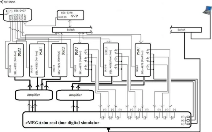
Figure 3.1 below shows a general overall system diagram depicting system layout with all equipment used in the implementation.

(27)

17

Figure 3.1: Overall system diagram.

The IEEE 9-bus WSCC system model is built using MATLAB SIMULINK and the load flow results is verified using ETAP software. The system is simulated in real-time using eMEGAsim Real-Time Digital Simulator OP5600. The voltages signals of load buses (bus-5, 6, 8) and three generator buses (bus 1, 2, 3) are sent via eMEGAsim analog output ports to the amplifiers. This is due to the voltage level limitation of only +16V the analog output ports can deliver, whereas the nominal secondary bus voltages are higher than that (e.g. 67V or 115V). Hence, the voltages signals are scaled down to the analog output ports level then scaled up by the amplification factor of the amplifier for the PMUs to receive. As shown in Figure 3.1, each of the six PMUs is assigned to a specific bus.

(28)

18

The PMUs measure the bus voltages, frequency, and rate of change of frequency which will then be sent to the SVP where the load shedding algorithm is programmed. Based on the received PMUs measurements and programmed algorithm, the SVP issues load shedding trip signals back to the load buses relays using the fast operate commands. Furthermore, the relay output contacts close based on the received trip signal from the SVP and the digital input in the eMEGAsim assigned to the asserted output contact - sheds the load in real-time. The upcoming sections will go through each step in more detail.

3.1.2 Hardware Used In Implementation

1. eMEGAsim Real-Time Digital Simulator OP5600 OPAL-RT System: real-time digital simulator.

2. F6350 Doble Amplifiers: to scale up the signals delivered by the analog outputs of the eMEGAsim.

3. SEL-2407: GPS clock source.

4. Six SEL-487E relays: used as PMUs.

5. SEL-3387 SVP: used as a central processing unit.

3.2 The IEEE WSCC 9-Bus System Model and Its Simulation In The Real-Time:

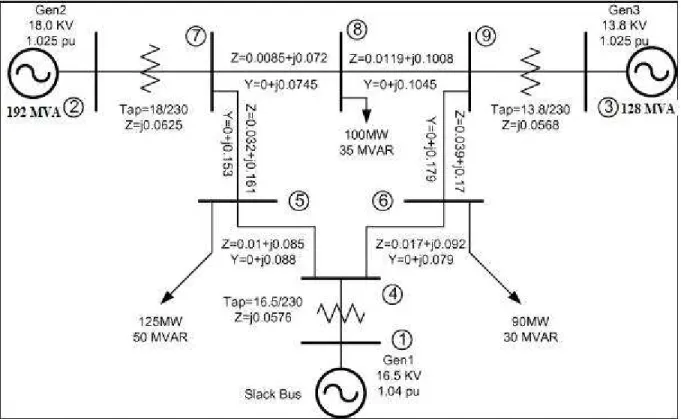
The studied system, IEEE WSCC 9-Bus system, has 3 generators and 3 load buses as shown on Figure 3.2.

(29)

19

Figure 3.2 IEEE 9-Bus system single line diagram

In this system, the voltage is 230kV and total load is 315MW. The loads at the load buses are divided into 20% large induction motors, 45% small induction motors, and 35% static load. This load allocation allows for an aggregate load model that reflects the dependency of the bus load to changes in voltage and frequency. Furthermore, table 3.1 shows the load divisions at each bus and the system data are attached to appendix A.

Table 3.1 Load divisions at load buses

Load bus Large induction motor

load

Small induction motor load Static load

Bus-5 25+j10 56.25+j22.5 43.75+j17.5

Bus-6 18+j6 40.5+j13.5 31.5+j10.5

(30)

20

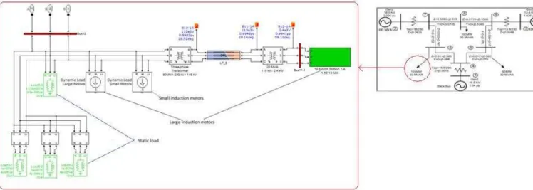
MATLAB SIMULINK has an induction motor block that contains large induction motor data that is included in appendix B. Similarly, there is a dynamic load block that has changeable variables to simulate different load type behaviors, such as air conditioner load, lighting loads, small industrial loads, large industrial loads. In this model, the dynamic load block is used for a small industrial motor load and the data for this block is taken from [16]. [16] examines different parameters for the dynamic load to achieve different load behaviors. For example, Figure 3.3 shows bus-5 load combination in SIMULINK.

Figure 3.3 Aggregate load at bus-5

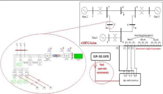
The static load at each bus is then divided into three feeders, where each feeder has a 10MW load. Each feeder is assigned to a specified digital input that is connected to the load bus relay output contact, as shown in Figure 3.4. Thus, the load is tripped in real-time upon the assertion of its related digital input, each digital input is asserted upon the assertion of its assigned output contact, and each output contact is asserted upon the receiving of the tripping signal from the SVP.

(31)

21

Figure 3.4 Assignment of eMEGAsim digital inputs with load feeders and relay output contacts for bus-5

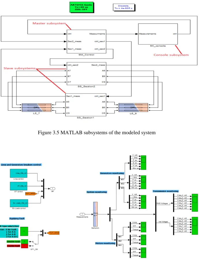
In order to appropriately simulate in real-time using eMEGAsim digital simulator, the system network is divided into four subsystems. As shown in Figure 3.5, the four subsystems and their purposes are as follows:

- The master subsystem: handles the sending of system measurements to the console and receiving the control signals from the console.

- The two slave subsystems: contains system network.

- The console subsystem: monitors and controls the system breakers.

As depicted in Figure 3.6, the console subsystem will, while the system is running, enable the changes of the system status in real-time; e.g., tripping a generator off or applying fault.

(32)

22

Figure 3.5 MATLAB subsystems of the modeled system

(33)

23

The three phase voltage signals at load buses and phase-A voltage signal at each generator bus are sent via the analog output ports to the amplifiers. Those signals are then multiplied by a gain value to guarantee that they will not exceed the output board voltage limit. This gain value is set based on the amplifier’s amplification factor and relay’s Voltage Transformer (VT) ratio in order to have the rated bus voltage value sent to the SVP.

3.3 Amplifiers

As described in the previous section, the eMEGAsim output voltage signals are scaled down by a gain value inside the model which prevents the output signal from exceeding the maximum voltage level of the analog output board. These low level voltage signals must be raised back to the rated secondary values before going into the relays (PMUs). Consequently, the Doble amplifier F6350 amplifies the low level analog signals which are then applied to the PMUs. Furthermore, Figure 3.7 shows the connections between the eMEGAsim and amplifiers.

(34)

24

Figure 3.7: Connections between eMEGAsim analog outputs-Amplifier-Relays.

There are several possible combinations that can be configured in F6350 amplifiers using F6 Multiple Amplifier Configurator software. For example, the user can choose three voltages and currents (3V & 3I), six voltages and currents (6V & 6I), the (6V & 6I) combination is the maximum available on this amplifiers. The six voltages and currents (6V & 6I) combination is chosen for this implementation, along with a source range of 75. This source range of 75 signifies that 6.7V low level input corresponds to 75V at the amplifier’s terminal that is ready to be applied to the relay,whereas the current channels are disabled as shown in Figure 3.8.

(35)

25

Figure 3.8 6V & 6I Amplifier Configuration

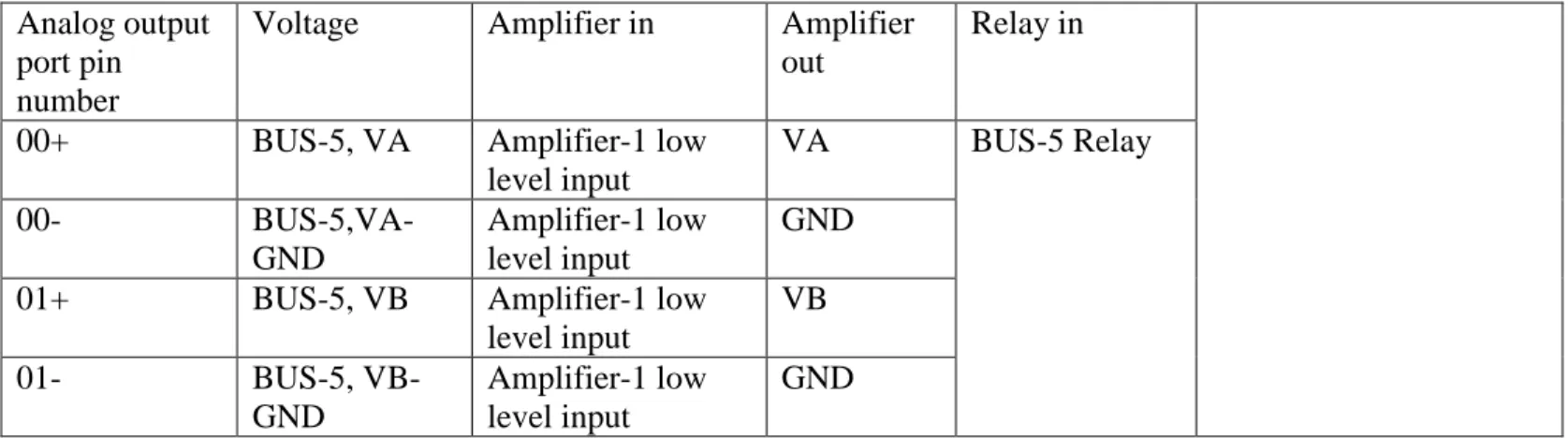
Pin assignments for the OPAR-RT analog output ports and amplifiers and also for the amplifiers and relays are depicted in Table 3.2.

Table 3.2 eMEGAsim analog output-amplifier-relay pin connections Analog output

port pin number

Voltage Amplifier in Amplifier

out

Relay in

00+ BUS-5, VA Amplifier-1 low

level input VA BUS-5 Relay 00- BUS-5,VA-GND Amplifier-1 low level input GND

01+ BUS-5, VB Amplifier-1 low

level input VB 01- BUS-5, VB-GND Amplifier-1 low level input GND

(36)

26 Table 3.2 continued

02+ BUS-5, VC Amplifier-1 low

level input VC 02- BUS-5, VC-GND Amplifier-1 low level input GND

level input VR 03- BUS-6,VA-GND Amplifier-1 low level input GND BUS-6 Relay

level input VS 04- BUS-6, VB-GND Amplifier-1 low level input GND

level input VT 05- BUS-6, VC-GND Amplifier-1 low level input GND

level input VA 08- BUS-8,VA-GND Amplifier-2 low level input GND BUS-8 Relay

level input VB 09- BUS-8, VB-GND Amplifier-2 low level input GND BUS-8 Relay

level input VC 10- BUS-8, VC-GND Amplifier-2 low level input GND

11+ GEN-2, VA Amplifier-2 low

level input VR 11- GEN-2,VA-GND Amplifier-2 low level input GND Gen-2 Relay

level input VS 12- GEN-3, VA-GND Amplifier-2 low level input GND Gen-3 Relay

level input VT 06_ GEN-1,VA GND Amplifier-2 low level input GND Gen-1 Relay

(37)

27 3.4 SEL-487E Relay

The Phasor Measurement Unit (PMU) in SEL-487E relays are utilized to send time synchronized measurements to the Synchrophasor Vector Processor (SVP). Moreover, all the relays are synchronized via the Satellite-Synchronized Clock SEL-2407 to allow for time stamped measurements as shown on Figure 3.9.

Figure 3.9 GPS and relay connection

The synchrophasor measurements are sent via an Ethernet port using the IEEE C37.118 protocol to the communication switch where the synchrophasor vector processor is connected. Hence, all therelays and SVP are on the same LAN. The UDP_T transport scheme is chosen for the load buses relays as the SVP can only send the control commands using UDP_T or UDP_S transport schemes. However, for the generator bus relays, the transport scheme is TCP as no control commands will be sent back to them by the SVP. The data traffic between the relays and

(38)

28

SVP is depicted in Figure 3.10. As each relay has a distinct ID, port number, and name, the SVP assigns each relay measurement according to the relay’s name and ID. Furthermore, the SVP requests the configuration block from each relay and automatically builds a database structure via the IEEE C37.118 protocol commands.

Figure 3.10 SVP and relays connections

The PMU has the capability to sample the measurements from 1 to 60 messages per second for 60 Hz system and from 1 to 50 messages per second for 50 Hz system. The full 60 messages/second in 60 Hz system is selected as a message rate in order to have accurate and close monitoring of the system behavior during the transient.

(39)

29

The positive sequence voltages from winding V in SEL-487E are selected to be sent from the load bus relays, and winding V phase voltages are selected to be sent from generator bus relays. This is due to the 3-phase voltage signals sent from the amplifier to the load bus relays and only 1-phase voltage signal sent from the amplifier to the generator bus relays. Hence, the only data points needed from the generator buses are their frequencies and rate of change of frequencies. All relays settings are attached to appendix C.

As shown in Figure 3.4, there are three output contacts in each load bus relay that connect to the digital input board of OPAL-RT to trip a specified amount of load which is determined by the SVP. Each output contact is asserted upon the assertion of the assigned remote bit coming from the SVP. The SVP can set/reset these remote bits if the relay is set to receive fast operate commands from the remote devices (SVP). The fast operate commands allow the host device (SVP) to initiate a control action without the need for a separate communication interface. For instance, when the fast operate command is enabled on the relay then it is easy to program the relay word bit (remote bits or circuit breaker bits) in the digital status word to observe the controlled function.

Table 3.3 shows the assignation of the relay output contacts with the remote bits. For example, if the SVP asserts RB01, the output contact OUT201 will close and the associated digital input port pin will be asserted and trip the connected load feeder in real-time.

Table 3.3 Assignment of remote bits with output contacts

Output Setting

OUT201 RB01 (remote bit 1)

OUT202 RB02 (remote bit 2)

(40)

30 3.5 Synchrophasor Vector Processor SVP

The Synchrophasor Vector Processor (SVP) SEL-3378 allows the use of synchronized phasor measurements (synchrophasors) for real-time power system monitoring, control, and protection. The SEL-3378 acquires and time correlates synchrophasor data from various Phasor Measurement and Control Units (PMCUs), such as SEL-421, SEL-487E, and SEL-411L relays. The SEL-3378 receives synchrophasor messages through serial and Ethernet communications. The SEL-3378 can process incoming data from as many as 20 PMCUs at a maximum data rate of 60 messages per second. The SVP can be configured to send control commands to external devices.

In this implementation, the SVP represents the central processing unit and contains the load shedding algorithm described in the last chapter. The algorithm is programmed using the SVP Configurator software. The SVP is programmed to collect the measurements from all relays (PMUs), time align these measurements and use the measurements to assess the system frequency stability. Additionally, the SVP calculates the amount of power to be shed, distributes this power among the load buses according to their voltage dip, and asserts the required number of remote bits using the fast operate command to their associated relays to trip the power needed to return the frequency to a safe level.

The SVP Configurator software offers five programming languages that comply with the requirements of IEC 61131-3. In this implementation, the ST (Structured Text) language is used to program the function blocks and CFC (Continuous Function Chart Editor) graphical language is used to assemble the function blocks that carry out the required algorithm calculations and decision making.

(41)

31

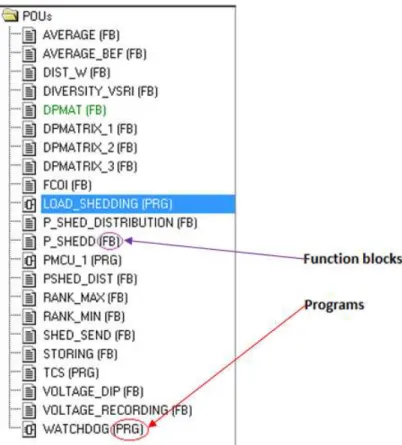
The Program Organization Unit (POU) used has 4 programs and more than ten programmed function blocks as shown in Figure 3.11. The SVP Configurator software executes these programs according to their assigned priority that is defined by the user and within a specified time interval.

Figure 3.11 POU of the Programmed algorithm

(42)

32

Figure 3.12 The interactions between POU programs in the SVP

The role of each program is as follows: 1. TCS (Time Alignment Client Server)

The TCS configuration is needed to enable the receiving from external servers (PMUs measurements) and send to external clients (sending shed commands back to the PMUs) synchrophasor messages and commands. This function is provided by Schweitzer Engineering Laboratories (SEL) within the baseline programming.

2. PMCU_1 (Phasor Measurement and Control Unit Input)

This function enables accessing the PMCU data from the TCS. This program has the highest priority as it contains the assignment of each PMU with its ID and name, creates a database for each PMU, and passes PMU data to other programs. Additionally, its time interval is 17ms as all the relays have message rates of 60msg/s; i.e. all relays send 1 message every 16.6ms. This function is provided by SEL within the baseline programming.

(43)

3. WATCHDOG

Each time this program

runs within an interval of 3s. If the watchdog does not reset within 3s, the watchdog will cause SEL-3378 to reset, along with the assertion of the alarm contact to notify the operator that there is a problem within the device. This function is provided by SEL within the baseline programming.

4. LOAD_SHEDDING (the load shedding scheme program)

This program is specially built to perform the load shedding algorithm and has function blocks that are no

highest priority as it contains calculations that depend on the data coming from PMUs and it has to run in the same time interval as PMCU_1 to ensure real

assessment. Furthermore, this

program code associated with all the functions blocks is included in appendix D.

Figure 3.13

33

this program runs, the watchdog is reset. It has the lowest priority and runs within an interval of 3s. If the watchdog does not reset within 3s, the watchdog will 3378 to reset, along with the assertion of the alarm contact to notify the is a problem within the device. This function is provided by SEL within the baseline programming.

LOAD_SHEDDING (the load shedding scheme program)

This program is specially built to perform the load shedding algorithm and has function blocks that are not provided by SEL. Similar to PMCU_1, this program has the highest priority as it contains calculations that depend on the data coming from PMUs and it has to run in the same time interval as PMCU_1 to ensure real

assessment. Furthermore, this program performs the tasks listed in Figure 3.13 and the program code associated with all the functions blocks is included in appendix D.

Figure 3.13 Load shedding scheme program flow

runs, the watchdog is reset. It has the lowest priority and runs within an interval of 3s. If the watchdog does not reset within 3s, the watchdog will 3378 to reset, along with the assertion of the alarm contact to notify the is a problem within the device. This function is provided by SEL

This program is specially built to perform the load shedding algorithm and has t provided by SEL. Similar to PMCU_1, this program has the highest priority as it contains calculations that depend on the data coming from PMUs and it has to run in the same time interval as PMCU_1 to ensure real-time system program performs the tasks listed in Figure 3.13 and the program code associated with all the functions blocks is included in appendix D.

(44)

RESULTS

The last chapter covers the station hardware setup to test the implemented a centralized adaptive UFLS. This chapter explains the test cases and system response for each case. The purpose of the test cases is to both examine the hardware functionality duri

disturbance with and without load shedding and evaluate the algorithm adaptability and SVP response for different disturbance locations. Additionally, Appendix E contains the results of the SVP for clarity.

4.1 Test Case-1: Generator-1 Outage

Generator-1 - producing 109MW

from the counsel subsystem as shown in Figure 4.1, table 4.1 shows the initial loading of generators before disturbance.

Figure 4.1

34 CHAPTER 4

RESULTS AND DISCUSSION

The last chapter covers the station hardware setup to test the implemented a centralized adaptive UFLS. This chapter explains the test cases and system response for each case. The purpose of the test cases is to both examine the hardware functionality duri

disturbance with and without load shedding and evaluate the algorithm adaptability and SVP response for different disturbance locations. Additionally, Appendix E contains the results of the

1 Outage with Initial Loading of 109MW

producing 109MW - was tripped off in real-time by opening its breaker from the counsel subsystem as shown in Figure 4.1, table 4.1 shows the initial loading of

Figure 4.1 System single line diagram for test case-1

The last chapter covers the station hardware setup to test the implemented a centralized adaptive UFLS. This chapter explains the test cases and system response for each case. The purpose of the test cases is to both examine the hardware functionality during a system disturbance with and without load shedding and evaluate the algorithm adaptability and SVP response for different disturbance locations. Additionally, Appendix E contains the results of the

time by opening its breaker from the counsel subsystem as shown in Figure 4.1, table 4.1 shows the initial loading of

(45)

35 Table 4.1 Initial generators loading for case-1

Generator-1 109MW

Generator-2 163MW

Generator-3 85MW

4.1.1 SVP Operation and Shedding Signals

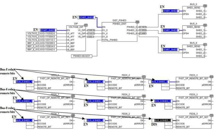
As a result of test case-1 scenario, the SVP estimated the mismatch power to be 88MW. Consequently, it distributed the amount of power to be shed among the load buses based on their voltage dip and sent the tripping signals by asserting the required remote bits on each relay. Figure 4.2 shows the operation of the SVP, where the blue/EN highlights indicate assertions and black/DIS highlights indicate de-assertions.

Figure 4.2 SVP estimation and distribution of the power to be shed among the load buses for case-1

(46)

36

The SVP made the decision to shed 34MW from bus-5, 33MW from bus-6, and 21MW from bus-8. As it was previously mentioned, each load bus was divided into three 10MW feeders. On the other hand, the SVP is programmed to shed the whole feeder if it has to shed between 5MW and 10MW. Hence, the SVP shed 3 feeders from bus-5, 3 feeders from bus-6, and 2 feeders from bus-8, as shown in Figure 4.2. Moreover, Figure 4.3 shows the relays output contact assertions and Figure 4.4 shows the MATLAB plot for each load feeder and eMEGAsim digital input signal status that was received from each load bus relay output contact.

(47)

37

Figure 4.4 The MATLAB plot of digital input status of the eMEGAsim

4.1.2 Disturbance Power

The disturbance power was estimated and plotted using MATLAB as shown in Figure 4.5. As depicted in this graph, the initial disturbance power is 79MW, which differs from the SVP’s earlier estimation of 88MW. The difference in the estimations between MATLAB simulation tool and SVP hardware is due to the difference in the df/dt seen by each one. The df/dt directly affects the estimation of the disturbance power as discussed in chapter two -- equation 2.1.

(48)

38

Figure 4.5 MATLAB estimation of the disturbance power

Furthermore, Figure 4.6 compares the df/dt sent from generator-2 PMU to the SVP and generator-2 df/dt from MATLAB. From this figure, both plots show a similar behavior but they are not identical. Thus, this difference in the rate of change of frequency seen by each tool participates in the disturbance power estimation mismatch.

Disturbance occurred

Load shedding scheme worked

(49)

39

Figure 4.6 Comparison between df/df seen by the SVP and df/dt from MATLAB

4.1.3 Frequency Response

The system frequency behavior was observed with and without applying the implemented load shedding scheme. The system frequency started to decline when the disturbance occurred. However, as soon as the load shedding scheme engaged and dropped the

(50)

40

required load to be shed, the frequency restored and settled close to the nominal frequency value as shown in Figure 4.7.

Figure 4.7 System frequency when applying the load shedding scheme

Alternatively, the system frequency declined below 50Hz for about 3s without applying load shedding and settled at about 54Hz as shown in Figure 4.8. In the real field when the frequency drops below pre-specified manufacturer value, the generator will trip off under the under-frequency generator protection after an intentional time delay. As a result, the frequency will decline sharply and the system blackout may probably occur.

(51)

41

Figure 4.8 System frequency without load shedding

4.1.4 Machines Active Power

Figure 4.9 shows the active power response for generators 2, 3, and their sum when the load shedding scheme was applied. As the disturbance occurred, the MW loading of each generator increased to share the loading of the tripped generator load, as each generator electrical loading increased beyond the mechanical loading the frequency is going to decline as shown on (Figure 4.7). However, as the load shedding scheme engaged soon as after the disturbance, the generator electrical overload was alleviated and generators almost returned to pre-disturbance loading.

(52)

42

Figure 4.9 Active power response for generator 2 and 3 by applying load shedding scheme

Alternatively, when lacking load shedding, generators 2 and 3 became heavily loaded as shown in Figure 4.10.

Figure 4.10: Active power response for generator 2 and 3 without load shedding. Disturbance

occurred

(53)

43 4.1.5 Load Buses Voltages

As loads at the load buses are composite of dynamic and static loads, their voltages change as the system changes. Figure 4.11 shows the voltages at the load buses when applying load shedding scheme. For this disturbance (generator-1 outage), bus-5 and 6 voltages were less than bus-8 after the disturbance as they were close to the tripped generator. Consequently, the SVP decided to shed more load from them in order to prevent any possible further voltage problems. As this load dropped from the system, the voltages at the load buses improved and settled close to their nominal pre-disturbance values.

Figure 4.11 Load buses voltage characteristics when applying load shedding

However, when lacking load shedding, bus-5 and 6 experienced more voltage drop than bus-8 immediately after the disturbance as shown in Figure 4.12. Ultimately, they settled on

(54)

44

values less than their nominal; i.e. 5 and 6 voltages were at about 210KV (0.91 p.u) and bus-8 voltage was at about 225KV (0.9bus-8 p.u).

Figure 4.12 Load buses voltage characteristics without load shedding

4.1.6 Machines Reactive Power

Figure 4.13 shows the reactive power of generators 2, 3, and their sum when load shedding scheme was applied. As the disturbance occurred, their MVAR output immediately increased as they tried to compensate for generator-1 MVAR loss. However, as the load shedding scheme engaged, each generator MVAR output started to decrease and settled near to its pre-disturbance MVAR output.

(55)

45

Figure 4.13 Reactive power with load shedding

Alternatively, when lacking the load shedding scheme, generators 2 and 3 MVAR output settled almost at three times the normal loading before the disturbance as in Figure 4.14. Furthermore, as the automatic voltage regulator (AVR) of these machines hits the maximum limits, system voltage instability will most probably occur.

(56)

46

Figure 4.14 Reactive power without load shedding

4.2 Test Case-2: Different Disturbance Locations

As mentioned earlier, among the goals of the test cases is to examine the adaptability of load shedding scheme via observing the SVP response for different disturbance locations. Test case-2 evaluates the following different system disturbances:

1. Case-2_I: Generator-1 outage with initial loading of 80MW. 2. Case-2_II: Generator-2 outage with initial loading of 80MW. 3. Case-2_III: Generator-3 outage with initial loading of 80MW.

4.2.1 Case-2_I: Generator-1 Outage with Initial Loading of 80MW

This disturbance was applied in real-time by opening generator-1 breaker from the console subsystem. Figure 4.15 shows the system breaker statuses during this disturbance, table 4.1 shows the initial loading of generators before disturbance.

(57)

Figure 4.15 System breakers statuse

Table 4.2 Initial generators loading for case Generator-1

Generator-2 Generator-3

The SVP estimated the disturbance power to be 42.7 MW, as shown in Figure 4.16. Furthermore, the SVP decided to shed 16.6MW from bus

from bus-8. Thus, it tripped 2 feeders from bus

47

System breakers statuses for case-2 generator-1 outag

Initial generators loading for case-2_I

80MW 170MW 108MW

The SVP estimated the disturbance power to be 42.7 MW, as shown in Figure 4.16. Furthermore, the SVP decided to shed 16.6MW from bus-5, 16.3MW from bus

8. Thus, it tripped 2 feeders from bus-5, 2 feeders from bus-6, and 1 feeder from bus 1 outage

The SVP estimated the disturbance power to be 42.7 MW, as shown in Figure 4.16. from bus-6, and 10.5MW 6, and 1 feeder from bus-8.

(58)

48

Figure 4.16 SVP estimation and distribution of the power to be shed among the load buses generator-1 outage 80MW

The system frequency started to decline when the disturbance occurred. However, as soon as the load shedding scheme dropped the required load to be shed, the frequency is restored and settled close to the nominal frequency value as shown in Figure 4.17.

(59)

49

Figure 4.17 System frequency for case-2 generator-1 outage

As shown in Figure 4.18, the voltages at load bus-5 and 6 experienced a drop when the disturbance occurred. This drop was more than the voltage drop at bus-8. Consequently, after the load shedding scheme worked the load buses voltage improved and settled close to their pre-disturbance nominal values.

(60)

Figure 4.18 Load bus voltages for case

4.2.2 Case-2_II: Generator-2 Outage w This disturbance was applied in

console subsystem. Figure 4.19 shows the system breakers statuses for this disturbance; table 4.3 shows the initial generators loading before disturbance.

Figure 4.19 System breakers statuse 50

Load bus voltages for case-2 generator-1 outage

2 Outage with Initial Loading of 80MW

This disturbance was applied in real-time by opening generator-2 breaker from the console subsystem. Figure 4.19 shows the system breakers statuses for this disturbance; table 4.3 shows the initial generators loading before disturbance.

System breakers statuses for case-2 generator-2 outage

2 breaker from the console subsystem. Figure 4.19 shows the system breakers statuses for this disturbance; table 4.3

(61)

51 Table 4.3 Initial generators loading for case-2_II

Generator-1 193MW

Generator-2 80MW

Generator-3 85MW

The SVP estimated the disturbance power to be 61 MW, as in Figure 4.20. Furthermore, the SVP decided to shed 17.5MW from bus-5, 11.5MW from bus-6, and 32MW from bus-8. Hence, it tripped 2 feeders from bus-5, 1 feeder from bus-6 and 3 feeders from bus-8.

(62)

52

The system frequency started to decline when the disturbance occurred. However, as soon as the load shedding scheme tripped the required load to be shed, the frequency restored and settled near the nominal frequency value as shown in Figure 4.21.

As shown in Figure 4.22, load bus-8 experienced more voltage drop than load bus-5 when the disturbance occurred and bus-5 experienced more voltage drop than bus-6. In another words, bus-8 voltage was the most affected bus after this disturbance, whereas bus-6 voltage was the least affected. Consequently, as the load shedding scheme worked, the load buses voltage improved and settled close to their nominal values before the disturbance.

(63)

Figure 4.22 Load

4.2.3 Case-2_III: Generator-3 Outage w The disturbance was applied in real

console subsystem. Figure 4.23 shows the system breakers statuses for this disturba shows the initial generators loading before disturbance.

Figure 4.23 System breakers statuses for case 53

Load bus voltages for case-2 Generator-2 outage

3 Outage with 80MW

The disturbance was applied in real-time by opening generator-3 breaker from the console subsystem. Figure 4.23 shows the system breakers statuses for this disturba

shows the initial generators loading before disturbance.

System breakers statuses for case-2 generator-3 outage

3 breaker from the console subsystem. Figure 4.23 shows the system breakers statuses for this disturbance, table 4.4

(64)

54 Table 4.4 Initial generators loading for case-2_III

Generator-1 115MW

Generator-2 163MW

Generator-3 80MW

The SVP estimated the disturbance power to be 60MW as shown in Figure 4.24. Moreover, the SVP decided to shed 8MW from 5, 18MW from 6, and 33MW from bus-8. Thus, it tripped 1 feeder from bus-5, 2 feeder from bus-6 and 3 feeders from bus-bus-8.

The system frequency started to decline when the disturbance occurred. However, as soon as the load shedding scheme tripped the required load to be shed, the frequency restored and settled near the nominal frequency value as shown in Figure 4.25.

(65)

55

As shown in Figure 4.26, when the disturbance occurred, voltage at bus-8 experienced more drop than voltage at bus-6 which dropped slightly more than voltage at bus-5. After the load shedding scheme worked the load buses voltages improved and settled almost close to their nominal values before the disturbance

(66)

56

Figure 4.26 Load bus voltages for case-2 Generator-3 outage

4.2.4 Comparison

Table 4.5 summarizes the results of test case-2. From this table, it is obvious that the SVP estimated a different disturbance power and distributed this power differently in each disturbance case. The SVP shed more power from the load buses that were nearby the disturbance location, as these load buses experienced higher voltage dip than those farther away from the disturbance location.

Table 4.5 Comparison between test results of case-2 Disturbance SVP estimated disturbance power Bus-5 tripped feeders Bus-6 tripped feeders Bus-8 tripped feeders Actual shed power Case-2_I 42.7MW 2 2 1 50MW Case-2_II 61MW 2 1 3 60MW Case-2_III 59.7MW 1 2 3 60MW

(67)

57 CHAPTER 5

CONCLUSION AND FUTURE WORK

5.1 Conclusion

This study objective is to use industrial grade hardware in the implementation of a central adaptive UFLS algorithm that aims to maintain system frequency stability and prevent voltage instability. This algorithm uses the frequency and rate of change of frequency to estimate the amount of power to be shed subsequent to an active power imbalance. Consequently, it distributes this power among the load buses based on their voltage dip during the disturbance. The study utilized an IEEE 9-bus system to test the algorithm, along with the eMEGAsim real time digital simulator, amplifiers, GPS, PMUs, and SVP equipments to form a complete hardware test-bed for the implementation.

The hardware used in the implementation responded as expected with the algorithm. Moreover, the PMUs sent the synchronized measurements they received from the eMEGAsim digital simulator. Additionally, the SVP received these measurements, performed the programmed load shedding algorithm, and issued the shedding signals accordingly. The interactions among all hardware together with the algorithm led to a satisfactory performance. Furthermore, the SVP decisions were able to restore system frequency to a safe level and improve voltage level at the load buses for each disturbance. Besides, the SVP was able distribute the amount of power to be shed according to the disturbance locations. This emphasizes the algorithm adaptability and also its suitability for the implementation in industry.

(68)

58

On other hand, the load model was able to reflect the load dependency on the voltage and frequency variations.

The testing showed a slight difference in the rate of change of frequency between the MATLAB simulation and the PMU hardware. This shows the importance of utilizing industrial grade hardware in testing new developed schemes, as it provides closer results to those faced in the field. Such a slight difference between hardware and software may result in the ma