Learning Tractable Multidimensional Bayesian Network Classifiers
Marco Benjumeda [email protected]
Concha Bielza [email protected]
Pedro Larra ˜naga [email protected]
Computational Intelligence Group Departamento de Inteligencia Artificial Universidad Polit´ecnica de Madrid, Spain
Abstract
Multidimensional classification has become one of the most relevant topics in view of the many domains that require a vector of class values to be assigned to a vector of given features. The popularity of multidimensional Bayesian network classifiers has increased in the last few years due to their expressive power and the existence of methods for learning different families of these models. The problem with this approach is that the computational cost of using the learned models is usually high, especially if there are a lot of class variables. Class-bridge decomposability means that the multidimensional classification problem can be divided into multiple subproblems for these models. In this paper, we prove that class-bridge decomposability can also be used to guarantee the tractability of the models. We also propose a strategy for efficiently bounding their inference complexity, providing a simple learning method with an order-based search that obtains tractable multidimensional Bayesian network classifiers. Experimental results show that our approach is competitive with other methods in the state of the art and ensures the tractability of the learned models.
Keywords: Multidimensional classification; Bayesian network classifiers; MPE complexity; learning from data.
1. Introduction
Classification is one of the main problems in machine learning nowadays. It consists of identifying to which class an instance described by a set of features belongs. Such an instance must often be assigned to a set of classes instead of to a single class. This is called multidimensional classification. This problem is common in several domains like text categorization (a text can be assigned to multiple topics), medicine (a patient may suffer from several diseases) or system monitoring (a system may break down from multiple failures).
Multidimensional Bayesian classifiers (MBCs) (van der Gaag and de Waal, 2006) extend Baye-sian network classifiers to the problem of multidimensional classification. An MBC is a BayeBaye-sian network (BN) whose structure is partitioned into three subgraphs: a class subgraph, a feature sub-graph, and a bridge subgraph (see below). The popularity of MBCs has grown in the last few years because of their good performance in multiple domains and their expressive graphical representa-tion, which explicitly shows the relationships among the variables of the models.
The main problem with using MBCs is that classification can be very computationally demand-ing to perform, especially for large sets of variables. To address this problem, Bielza et al. (2011) proposed a class of MBCs, called class-bridge decomposable (CB-decomposable) MBCs, whose structure can be decomposed into multiple connected components, omitting the arcs between the
features. In this paper, we demonstrate that MBCs can perform classification efficiently if the num-ber of class variables in each of their components is bounded. We also propose a method for learning tractable MBCs from data.
The rest of the paper is organized as follows. Section 2 includes the description of CB-decompo-sable MBCs and reviews inference complexity and previous work on MBCs. Section 3 presents the results with respect to the complexity of classification in MBCs, and describes the method proposed for learning tractable MBCs. Section 4 reports the experimental results. Section 5 gives our conclusions and suggests future research lines.
2. Background
2.1 Multidimensional Bayesian Network Classifiers
A Bayesian networkBrepresents a joint probability distribution over a set of random variablesV =
{V1, . . . , Vn}. It is composed of a directed acyclic graph (DAG)G that represents the conditional
dependences among the variables inV, and a set of parameters Pr(Vi|PaG(Vi))(we usePaG(Vi)to
refer to the parents ofViinG) that represent the conditional probability distributions (CPDs) of each
Vi∈ V conditioned on its parents inG. The joint probability distribution encoded byBis given by
Pr(V1, . . . , Vn) = n
Y
i=1
Pr(Vi|PaG(Vi)) . (1)
Van der Gaag and de Waal (2006) introducedmultidimensional Bayesian network classifiersas an extension of Bayesian classifiers to multidimensional classification. MBCs are a special case of Bayesian networks with a restricted structure topology. They are defined as follows:
Definition 1 An MBC is a Bayesian networkBover a set of variablesV ={V1, V2, . . . , Vn}, where
Vis partitioned into two setsC ={C1, . . . , Cd},d≥1, of class variables andF ={F1, . . . , Fm},
m≥1, of feature variables (d + m = n). The arcs inGare partitioned into three subsets,AC,AF,
AB, such that:
• AC ⊆ C × Cis composed of the arcs between the class variables having a subgraphGC =
(C, AC)–class subgraph– ofGinduced byC.
• AF ⊆ F × F is composed of the arcs between the feature variables having a subgraph
GF = (F, AF)–feature subgraph– ofGinduced byF.
• AB ⊆ C ×Fis composed of the arcs from the class variables to the feature variables having a
subgraphGB = (V, AB)–bridge subgraph– ofGinduced byV connecting class and feature
variables.
Figure 1 shows an example of the structure of an MBC and its corresponding subgraphs. An MBC performs classification by obtaining the most probable explanation (MPE) of the class variables given an instance of the feature variables, which is given by
c∗ =argmaxc∈ΩCPr(c|f) =argmaxc∈ΩCPr(c,f) , (2) wherefis an instance ofFandΩCare the possible configurations ofC.
C1 C2 C3 C4 C5 F1 F2 F3 F4 F5 F6 Class subgraph C1 C2 C3 C4 C5 Bridge subgraph C1 C2 C3 C4 C5 F1 F2 F3 F4 F5 F6 Feature subgraph F1 F2 F3 F4 F5 F6 Figure 1: MBC structure
2.2 Class-Bridge Decomposable Multidimensional Bayesian Network Classifiers
Bielza et al. (2011) introducedclass-bridge decomposable multidimensional Bayesian network clas-sifiers, a type of MBCs that can be decomposed into multiple connected components, where there are no arcs belonging to the class or bridge subgraphs that connect two nodes in two different com-ponents.
Definition 2 A CB-decomposable MBC is a BNBwhose class subgraph and bridge subgraph are decomposed intormaximal components such that:
1. GC ∪ GB = Sri=1(GCi ∪ GBi), where GCi ∪ GBi,i = 1, . . . , r, are its maximal connected
components.
2. ChG(Ci)∩ChG(Cj) =∅, withi, j= 1, . . . , randi6=j, whereChG(Ci)andChG(Cj)denote
the children of all variables inCi andCj respectively (the subsets of class variables in GCi andGCj).
Bielza et al. (2011) showed that exploiting the CB-decomposability of MBCs can reduce the number of computations required to perform multidimensional classification. Specifically, they showed that the MPE can be computed independently in each component, given that
max c∈ΩCPr(c|f)∝ r Y i=1 max ci∈ΩCi Y C∈Ci Pr(c|PaG(C)) Y F∈ChG(Ci) Pr(f|PaGB(F),PaGF(F)) , (3)
which means that it is possible to maximize over each maximal connected component indepen-dently, therefore maximizing over lower dimensional spaces.
The MBC shown in Figure 1 classifies an instancef = (f1, . . . , f6)by obtaining the MPE of
(C1, . . . , C5) givenf. As this MBC can be CB-decomposed into two connected components (see
Figure 2), Equation (3) shows that the MPE can be computed maximizing over(C1, C2, C3)and
C1 C2 C3 C4 C5
F1 F2 F3 F4 F5 F6
Figure 2: Connected components of the MBC shown in Figure 1
2.3 Inference Complexity in Multidimensional Bayesian Network Classifiers
Assuming that all the feature variables are observed, performing classification in an MBCBwith class variables C = {C1, . . . , Cd} and feature variablesF = {F1, . . . Fm} is equivalent to
ob-taining the MPE of the class variables conditioned on an instance f of the features. If there are unobserved feature variables, performing classification inBis equivalent to obtaining not the MPE in(C1, . . . , Cd)but the maximum a posteriori hypothesis (MAP). This can be intractable even if the
treewidth ofBis bounded (Park, 2002).
Existing research addresses the complexity of multidimensional classification in MBCs as the complexity of computing the MPE. Thus, they implicitly assume that MPE queries will not contain missing values (i.e., the values of all the feature variables will be given). Otherwise the resulting MPE would provide the most probable instance not of(C1, . . . , Cd)but of(C1, . . . , Cd, Fm1, . . . ,
Fmk), whereFm1, . . . , Fmk are the missing features.
In this paper, we also focus on the case where all the feature variables are observed. Hence, we consider that, to perform classification, an MBC obtains argmaxc∈ΩCPr(c,f). MPE is generally
NP-hard (Kwisthout, 2011), but it can be computed in polynomial time in any BN if the treewidth of G is bounded (Sy, 1992), where G is the structure of B. Given MBC structural constraints, further bounds on their inference complexity have been found. De Waal and van der Gaag (2007) demonstrated that treewidth(G)≤treewidth(GF) +d, whereGF is the graph that contains the arcs
among feature variables anddis the number of class variables. This means that it is possible forB
to perform classification in polynomial time if the addition of the treewidth of the feature subgraph and the number of class variables is bounded. Furthermore, ifGis CB-decomposable the MPE can be computed in polynomial time if the treewidth ofGF and the number of class variables of each component ofGare bounded (Kwisthout, 2011).
Pastink and van der Gaag (2015) also suggested that the treewidth of an MBC with an empty feature subgraph is given by the treewidth of the graph obtained after moralizing its structure and then removing all its feature nodes from the moralized graph.
When computing the MPE in a BN given an evidencef, we can simplify the structure of the network by pruning every arcVi →Vj such thatViappears inf. Pruning arcVi →Vj for evidence
ffrom a BN means removing arcVi → Vj and the parameters ofVj that are not compatible withf.
When the MPE of the class variables is computed in an MBC, the values of all the feature variables are given.
As mentioned above, previous research uses the treewidth of G to bound the inference com-plexity, exploiting the restrictions on the topology ofG, but without considering the known query-dependent information, that is, that all the feature variables are instantiated when we compute the MPE inB. Here, we take advantage of the above to efficiently bound the complexity of multidi-mensional classification in MBCs.
2.4 Previous Work on Learning MBCs
The problem of learning MBCs from data has been addressed before. The literature contains meth-ods for learning different families of MBCs, depending on the type of class and feature subgraphs that they can obtain (trees, forests, polytrees or DAGs). Here we denote the family of the MBC using class subgraph – feature subgraph (e.g., tree–DAG has a tree as the class subgraph and a DAG as the feature subgraph).
Methods have been proposed for learning tree–tree (van der Gaag and de Waal, 2006), polytree– polytree (de Waal and van der Gaag, 2007) and DAG–DAG (Bielza et al., 2011) MBCs. These approaches do not explicitly consider the inference complexity of the learned models. Hence, they may lead to MBCs where the MPE cannot be solved efficiently, unless the numberdof class vari-ables is very small.
There are also other approaches in the literature that consider the complexity of the MBCs during the learning process. Corani et al. (2014) proposed a method for learning sparse MBCs with a forest class subgraph and an empty feature subgraph, and Borchani et al. (2010) introduced the first method to learn CB-decomposable MBCs, but neither of them provides guarantees regarding the complexity of multidimensional classification in the models. Pastink and van der Gaag (2015) proposed a method for learning tree–empty MBCs of bounded treewidth, providing an optional step to learn a forest feature subgraph, and guaranteeing the tractability of the resulting models. The method computes the treewidth of each candidate and rejects any that exceed the treewidth bound. Computing the treewidth of the models can be very computationally demanding, specially if we aim to learn (the most general) DAG–DAG MBCs.
In this paper we propose a strategy for efficiently bounding the inference complexity of CB-decomposable MBCs with DAG–DAG structure. We use this strategy to learn MBCs where the MPE can be computed in polynomial time. We show that even high treewidth MBCs perform classification efficiently if the number of class variables per component is bounded.
3. Learning Tractable MBCs
Given that inference in a BN is tractable if the treewidth of its structure is bounded, most existing algorithms for learning BNs with low inference complexity bound the treewidth of the networks during the learning process, rejecting any candidates that exceed the treewidth bound.
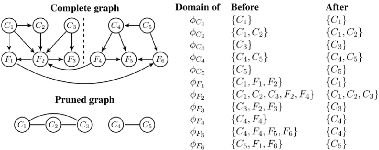
In the case of MBCs, it is possible to exploit the restrictions on the structure of the network and the information about the MPE queries sent to the MBCs. From the structure of MBCs, we know that there are no arcs from the feature to the class nodes. We also know that each MPE query sent to the network involves finding the most probable instance of the class variables given an instance of the features. The complexity of the MPE in BNs is query dependent, given that the parameters of a network can be updated with the value of the evidence variables before computing the MPE. Definition 3 LetG = (C ∪ F,AC ∪ AB∪ AF)be the structure of an MBCB. The pruned graph
ofGis the result of moralizingGand removing the feature nodes from the resulting graph.
Theorem 4 states that performing classification in an MBC is tractable if the treewidth of its pruned graph is also bounded. This transformation was used by Pastink and van der Gaag (2015) to bound the treewidth of tree–empty MBCs. Here, we use it to bound the complexity of multidimen-sional classification in DAG–DAG MBCs.
Complete graph
C1 C2 C3 C4 C5
F1 F2 F3 F4 F5 F6
Pruned graph
C1 C2 C3 C4 C5
Domain of Before After
φC1 {C1} {C1} φC2 {C1, C2} {C1, C2} φC3 {C3} {C3} φC4 {C4, C5} {C4, C5} φC5 {C5} {C5} φF1 {C1, F1, F2} {C1} φF2 {C1, C2, C3, F2, F4} {C1, C2, C3} φF3 {C3, F2, F3} {C3} φF4 {C4, F4} {C4} φF5 {C4, F4, F5, F6} {C4} φF6 {C5, F1, F6} {C5}
Figure 3: MBC structure and pruned graph (left), and domain of the potential of each node before and after they are updated with evidencef= (f1, . . . , f6)(right)
Theorem 4 LetG = (C ∪ F,AC ∪ AB∪ AF)be the structure of an MBCB. If the treewidth of
its pruned graphG0 and the number of parents of each node that belongs toFare bounded,Bcan perform classification in polynomial time.
Proof B performs classification by obtaining argmaxc∈ΩCPr(c,f), where f is an instance of F. Suppose that the CPD of each nodeVi ∈ C ∪ F is represented by a potentialφi.φiis updated with
fby removing the entries that are not compatible withf. This can be done in linear time in the size ofφi, that is exponential in the number of parents ofViinG. Hence, the nodes inFcan be updated
withfin polynomial time if the number of parents of each node inF is bounded.
After updating Gwithf, the domain of each potentialφf ofVf ∈ F isPaG(Vf)∩ C. There is
an undirected link inG0 between each node inPaG(Vf)∩ C. It is evident that the width of the best
elimination order for the resulting potentials is equal to the treewidth ofG0. Hence, if the treewidth ofG0 is bounded,Bcan perform classification in polynomial time.
Figure 3 shows an example of the structure of an MBC and its pruned graph. It also illustrates that all the variables belonging to the domain of the same potentialφi ∈ {φC1, . . . , φC5, φF1, . . . ,
φF6}updated with an instancef= (f1, . . . , f6)of the features are connected by a link in the pruned
graph (and vice versa). This means that the treewidth of the pruned graph is equal to the width of the best elimination order in the updated potentials.
Although the treewidth of this graphG0provides a tight upper bound on the inference complexity
of the models, computing the treewidth of a graph exactly is an NP-complete problem (Arnborg et al., 1987).
We can compute whether the treewidth of a graph is less than or equal to a constantkin linear time ifkis fixed, but obtaining the solution of this inequality is super-exponential in the treewidth (Bodlaender, 1993). Thus, it is intractable unlesskis very small.
Fortunately, Collorary 5 shows that if the number of class variables of an MBCBis bounded, then we can perform classification inBin polynomial time.
Corollary 5 LetG= (C ∪ F,AC∪ AB∪ AF)be the structure of an MBCB. If the number of class variablesdand the number of parents of each node inFare bounded,Bcan perform classification in polynomial time.
Proof LetG0be the pruned graph ofG. As each node inG0belongs toC, treewidth(G0)≤d. Hence, from Theorem 4 we know that if the number of parents of each feature anddare bounded,Bcan perform classification in polynomial time.
When the number dof class variables ofBis not small, it is not so simple to decide ifBcan perform classification efficiently. Nevertheless, if the classifier is CB-decomposable, we can show that simply bounding the maximum number of class nodes per component also bounds the inference complexity of the MBCs, as shown in Collorary 6.
Corollary 6 LetG = (C ∪ F,AC∪ AB∪ AB)be the structure of a CB-decomposable MBCB. If
the number of class variables in each component ofGand the number of parents of each node inF are bounded,Bcan perform classification in polynomial time.
Proof LetG0be the pruned graph ofG. IfGis CB-decomposable intorcomponentsG1, . . . ,Gr, then
G0is composed ofrunconnected subgraphsG0
1, . . . ,Gr0, such thatVi0 =Vi∩ C,i= 1, . . . , r, where
Vi andVi0 are the nodes inGi and Gi0, respectively. As treewidth(G0) = maxi{treewidth(G0i)} <
maxi|Vi0|= maxi|Vi∩ C|, we know from Theorem 4 that if the number of parents of each feature
and the number of class variables in each component ofGare bounded,Bcan perform classification in polynomial time.
Figure 3 shows that the treewidth of the pruned graph is bounded by the maximum number of class variables per component, given that there is no path fromCitoCj in the pruned graph if two
class nodesCiandCj are in two different connected components.
As it is straightforward to establish the number of class variables per component of an MBC, we can efficiently bound the inference complexity of MBCs during the learning process.
3.1 Learning Method
Next, we provide a method for learning CB-decomposable MBCs (with a DAG-DAG structure) that guarantees the tractability of the resulting models. In order to efficiently bound the inference complexity of classification, we limit the number of class variables per component. This strategy can be used in combination with most score+search methods.
We adapt order-based search (OBS) (Bouckaert, 1992) to learn tractable MBCs. As the order of the variables in greedy search restricts the structure of the learned networks (i.e., a node can only be set as the parent of another node if it has been visited previously), OBS can be easily adapted to learn MBCs by considering only those orderings of the variables where the class variables precede the feature variables. In this manner, the parents of class variables must necessarily be other class variables. This is consistent with the MBC structure.
To bound the inference complexity, we simply reject any candidates that exceed the bound of class variables per component. We use Algorithm 1 to learn the structure of MBCs given an ordering of the class (OC) and feature (OF) variables and a bound on the maximum number of class variables
per componentk. We do not specify a definite scoring function because any score used to evaluate BNs can be applied. We assume that the score must be maximized.
Data: DataD, ordering of class variablesOC, ordering of feature variablesOF, boundk
Result: MBC structureG 1 G ←empty DAG; 2 O←(OC,OF); 3 forVi∈O do 4 improve←true; 5 whileimprovedo
6 LetVj be the node that maximizes score(D, Vi,PaG(Vi)∪ {Vj}), such that addingVj
toPaG(Vi)does not exceed the boundkof class variables per component inG;
7 improve←false;
8 ifscore(D, Vi,PaG(Vi)∪ {Vj})>score(D, Vi,PaG(Vi))then
9 PaG(Vi)←PaG(Vi)∪ {Vj}; 10 improve←true; 11 end 12 end 13 end 14 returnG;
Algorithm 1:Greedy search of tractable CB-decomposable MBCs (CB–OBS)
An effective strategy used to learn BNs in the space of orderings is to perform a greedy process applying local changes among the orderings and picking the best change in each step (Teyssier and Koller, 2005). A tabu list can also be used to reduce the computational cost, and random restarts can be useful for avoiding local optima. We use this strategy to learn MBCs in the experiments.
4. Experimental Results
To test the performance of our approach, we compared it with other state-of-the-art methods, in-cluding the tree–tree (van der Gaag and de Waal, 2006), polytree–polytree (de Waal and van der Gaag, 2007) and pure filter (DAG–DAG) (Bielza et al., 2011) algorithms. We also compared it to a version of the method proposed by Pastink and van der Gaag (2015) (small–tw). Instead of the branch and bound approach that they propose, we learned the bridge subgraph using a greedy search process that picks the best parents set that does not exceed the treewidth bound in each iteration, given that the computational cost of the former is too high for this experimental framework. We used the Bayesian information criterion (BIC) as the scoring function for our method. CB–OBS will denote our approach.
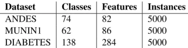
We generated a dataset of 5000 samples from three real-world BNs. ANDES (Conati et al., 1997) is an intelligent tutoring system for Newtonian physics, MUNIN1 (Andreassen et al., 1989) is a network for the diagnosis of neuromuscular disorders , and DIABETES (Andreassen et al., 1991) is an insulin adjustment system. We selected one third of the variables at random as class variables. To select the features, we applied an information gain filter for each of the classes, generating a subset of selected features for each class variable. The definitive subset of features is the union of the subsets selected for each variable. The basic properties of the datasets are described in Table 1.
Dataset Classes Features Instances
ANDES 74 82 5000
MUNIN1 62 86 5000
DIABETES 138 284 5000
Table 1: Basic properties of the datasets
Method τ τp size accM
CB–OBS 7.8±0.7 5.2±1.0 679±157 0.778±0.001∗
tree–tree 18.4±0.8 7.8±0.4 3710±724 0.779±0.002∗
polytree–polytree 21.8±2.4 8.2±0.4 5221±342 0.777±0.003 pure filter 25.2±1.2 9.2±1.2 8756±3542 0.776±0.003 small–tw 5.0±0.0 5.0±0.0 1382±171 0.764±0.004
Table 2: Performance of MBC methods in ANDES dataset
To test the performance of the methods, we used the mean accuracy of the classifiers, which averages the accuracies of all the class variables individually, as described for N samples andd classes below: accM = 1 d·N d X i=1 N X j=1 δ(c0ij, cij) , (4)
wherec0ij represents the predicted class label for variableCj in instancei,cij is its true value, and
δ(c0ij, cij) = 1ifc0ij =cij, and0otherwise.
4.1 Results
Tables 2–4 show the performance of the compared methods estimated with 5-fold cross-validation. For each dataset and method, we show the treewidth (τ) of the learned models, obtained using the Min-Fill algorithm, the treewidth (τp) of the pruned graph, the size of the factors induced by variable
elimination for solving the MPE, and the mean accuracy (accM). The time complexity of variable
elimination is given by the size of the induced factors. In all cases, the bound on the number of class variables per componentkwas set to15. Small values ofkusually returned MBCs with a very low treewidth, which detracts from classification accuracy, while big values ofkdid not guarantee the tractability of the learned MBCs. The bound in the treewidthτ for small–tw was set to5. Other small values of τ produced similar results. The best results are shown in bold, and we use ∗ to denote a statistically significant improvement with respect to small–tw.
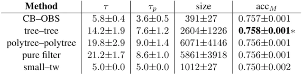
The treewidth and size of the pruned graphs (that bound the complexity of multidimensional classification in MBCs) obtained with CB–OBS and small–tw were smaller than for the models obtained with tree–tree, polytree–polytree and pure filter algorithms, especially in the case of the DIABETES dataset, where the MBCs learned by tree–tree, polytree–polytree and pure filter were unable to perform classification due to space and time limitations.
We compared the accuracy results in the ANDES and MUNIN1 datasets using a Friedman aligned ranks test withp < 0.05and Nemenyi’s and Holm’s procedures. Methods tree–tree and
Method τ τp size accM CB–OBS 5.8±0.4 3.6±0.5 391±27 0.757±0.001 tree–tree 14.2±1.9 7.6±1.2 2604±1226 0.758±0.001∗ polytree–polytree 19.8±2.9 9.0±1.4 6071±4146 0.756±0.001 pure filter 21.2±1.7 8.6±1.0 5861±3918 0.756±0.001 small–tw 5.0±0.0 5.0±0.0 1012±27 0.750±0.002
Table 3: Performance of MBC methods in MUNIN1 dataset
Method τ τp size accM
CB–OBS 72.2±2.9 5.4±0.5 2200±367 0.934±0.015∗
tree–tree 66.6±10.9 37.4±2.6 (5.183±8.999)×1012 −
polytree–polytree 100.6±8.0 54.4±5.7 (3.216±3.950)×1018 −
pure filter 93.0±3.2 55.8±2.5 (1.154±1.551)×1018 −
small–tw 5.0±0.0 5.0±0.0 2802±179 0.931±0.016
Table 4: Performance of MBC methods in DIABETES dataset
small–tw were found significantly different in all the datasets by both procedures, and CB–OBS and small–tw were also found significantly different in the ANDES dataset by both procedures.
As we only obtained accuracy results for CB–OBS and small–tw in the DIABETES dataset, we compared both methods using a Wilcoxon test with p < 0.05, and the results obtained with CB–OBS were found significantly better than the results obtained with small–tw.
Note that the treewidth of the pruned graph of the models was clearly smaller than the treewidth of the entire structure in some cases (see the results of CB–OBS in the DIABETES dataset). This shows that the treewidth of the networks does not have to be bounded to obtain MBCs whose MPE of the class variables can be computed efficiently.
5. Conclusions and Future Research
In this paper, we addressed the problem of the complexity of multidimensional classification in MBCs. We demonstrated that some MBCs can perform classification efficiently even if they have a large treewidth. We provided upper bounds for the complexity of the models. Also, we showed that CB-decomposability can be used to efficiently guarantee the tractability of MBCs. We proposed a learning method that uses the above properties to ensure such tractability.
Experimental results showed that the proposed method is competitive with other state-of-the-art methods in terms of accuracy, also ensuring that the learned MBCs can be solved efficiently. We also observed that some models remain tractable even with a large treewidth.
The upper bound provided by the number of class variables per component has the advantage of being able to be computed without increasing the computational cost of the learning process. However, there are MBCs that have a pruned graph with low treewidth and also have components with a high number of class variables. Thus, forcing the CB-decomposability of the models could lead to the rejection of some tractable models during the learning process. Although computing the treewidth for each candidate will often be an overkill, there are methods in the literature that learn
bounded treewidth BNs (Elidan and Gould, 2009; Chechetka and Guestrin, 2008). We intend to adapt these methods to learn MBCs where the treewidth of the pruned graph is bounded.
Finally, one of the main problems with models with latent variables is that exact inference usu-ally has to be performed during the learning process to complete the values of the hidden variables (e.g., structural expectation-maximization). We are interested in adapting the ideas described here to reduce the learning complexity of these models without restricting their structure to trees or poly-trees.
Acknowledgments
This work has been partially supported by the Spanish Ministry of Economy and Competitive-ness through the Cajal Blue Brain (C080020-09; the Spanish partner of the Blue Brain initiative from EPFL) and TIN2013-41592-P projects, by the Regional Government of Madrid through the S2013/ICE-2845-CASI-CAM-CM project, and by the European Union’s Seventh Framework Pro-gramme (FP7/2007-2013) under grant agreement no. 604102 (Human Brain Project). M. Ben-jumeda is supported by a predoctoral contract for the formation of doctors from the Spanish Ministry of Economy and Competitiveness (BES-2014-068637).
References
S. Andreassen, F. V. Jensen, S. K. Andersen, B. Falck, U. B. Kjærulff, M. Woldbye, A. R. Sørensen, A. Rosenfalck, and F. Jensen. MUNIN—an expert EMG assistant. Computer-aided Electromyo-graphy and Expert Systems, 21, 1989.
S. Andreassen, R. Hovorka, J. Benn, K. G. Olesen, and E. R. Carson. A model-based approach to insulin adjustment. Proceedings of the 3rd Conference on Artificial Intelligence in Medicine, pages 239–248, 1991.
S. Arnborg, D. G. Corneil, and A. Proskurowski. Complexity of finding embeddings in a k-tree.
SIAM Journal on Algebraic Discrete Methods, 8(2):277–284, 1987.
C. Bielza, G. Li, and P. Larra˜naga. Multi-dimensional classification with Bayesian networks. Inter-national Journal of Approximate Reasoning, 52(6):705–727, 2011.
H. L. Bodlaender. A linear time algorithm for finding tree-decompositions of small treewidth. In
Proceedings of the 25th Annual ACM Symposium on Theory of Computing, pages 226–234. ACM, 1993.
H. Borchani, C. Bielza, and P. Larra˜naga. Learning CB-decomposable multi-dimensional Bayesian network classifiers.Proceedings of the 5th European Workshop on Probabilistic Graphical Mod-els, pages 25–32, 2010.
R. R. Bouckaert. Optimizing causal orderings for generating dags from data. In Proceedings of the 8th International Conference on Uncertainty in Artificial Intelligence, pages 9–16. Morgan Kaufmann Publishers Inc., 1992.
A. Chechetka and C. Guestrin. Efficient principled learning of thin junction trees. InAdvances in Neural Information Processing Systems, pages 273–280, 2008.
C. Conati, A. S. Gertner, K. VanLehn, and M. J. Druzdzel. On-line student modeling for coached problem solving using Bayesian networks. In Proceedings of the 6th International Conference on User Modeling, pages 231–242. Springer, 1997.
G. Corani, A. Antonucci, D. D. Mau´a, and S. Gabaglio. Trading off speed and accuracy in multilabel classification. InProceedings of the 7th European Workshop on Probabilistic Graphical Models, pages 145–159, 2014.
P. R. de Waal and L. C. van der Gaag. Inference and learning in multi-dimensional bayesian net-work classifiers. InProceedings of the 9th European Conference on Symbolic and Quantitative Approaches to Reasoning with Uncertainty, pages 501–511. Springer, 2007.
G. Elidan and S. Gould. Learning bounded treewidth Bayesian networks. InAdvances in Neural Information Processing Systems, pages 417–424, 2009.
J. Kwisthout. Most probable explanations in Bayesian networks: Complexity and tractability. In-ternational Journal of Approximate Reasoning, 52(9):1452–1469, 2011.
J. D. Park. MAP complexity results and approximation methods. InProceedings of the 18th Con-ference on Uncertainty in Artificial Intelligence, pages 388–396. Morgan Kaufmann Publishers Inc., 2002.
A. Pastink and L. C. van der Gaag. Multi-classifiers of small treewidth. InProceedings of the 13th European Conference on Symbolic and Quantitative Approaches to Reasoning with Uncertainty, pages 199–209. 2015.
B. K. Sy. Reasoning MPE to multiply connected belief networks using message passing. In Pro-ceedings of the 10th National Conference on Artificial intelligence, pages 570–576. AAAI Press, 1992.
M. Teyssier and D. Koller. Ordering-based search: A simple and effective algorithm for learning Bayesian networks. InProceedings of the 21st Conference on Uncertainty in Artificial Intelli-gence, pages 584–590. AUAI Press, 2005.
L. C. van der Gaag and P. R. de Waal. Multi-dimensional Bayesian network classifiers. In Proceed-ings of the 3rd European Workshop on Probabilistic Graphical Models, pages 107–114, 2006.