Combining dissimilarity measures for prototype-based classification
Mwebaze, Ernest; Bearda, Gjalt; Biehl, Michael; Zuehlke, Dietlind
Published in:European Symposium on Artificial Neural Networks (ESANN) 2015
IMPORTANT NOTE: You are advised to consult the publisher's version (publisher's PDF) if you wish to cite from it. Please check the document version below.
Document Version
Publisher's PDF, also known as Version of record
Publication date: 2015
Link to publication in University of Groningen/UMCG research database
Citation for published version (APA):
Mwebaze, E., Bearda, G., Biehl, M., & Zuehlke, D. (2015). Combining dissimilarity measures for prototype-based classification. In M. Verleysen (Ed.), European Symposium on Artificial Neural Networks (ESANN) 2015 (Vol. 23, pp. 31-36). d-side publishing.
Copyright
Other than for strictly personal use, it is not permitted to download or to forward/distribute the text or part of it without the consent of the author(s) and/or copyright holder(s), unless the work is under an open content license (like Creative Commons).
Take-down policy
If you believe that this document breaches copyright please contact us providing details, and we will remove access to the work immediately and investigate your claim.
Downloaded from the University of Groningen/UMCG research database (Pure): http://www.rug.nl/research/portal. For technical reasons the number of authors shown on this cover page is limited to 10 maximum.
Combining dissimilarity measures for
prototype-based classification
Ernest Mwebaze1 and Gjalt Bearda2and Michael Biehl2 and Dietlind Z¨uhlke3 1- Makerere University, Department of Information Technology
Plot 56, Makerere University Pool Road, Kampala, Uganda. 2- University of Groningen, Johann Bernoulli Institute for
Mathematics and Computer Science P.O. Box 407, 9700 AK Groningen, The Netherlands 3- Fraunhofer Institute IAIS, Department of Organized Knowledge
Schloss Birlinghoven, 53757 Sankt Augustin, Germany
Abstract. Prototype-based classification, identifying representatives of the data and suitable measures of dissimilarity, has been used successfully for tasks where interpretability of the classification is key. In many practi-cal problems, one object is represented by a collection of different subsets of features, that might require different dissimilarity measures. In this paper we present a technique for combining different dissimilarity measures into a Learning Vector Quantization classification scheme for heterogeneous, mixed data. To illustrate the method we apply it to diagnosing viral crop disease in cassava plants from histograms (HSV) and shape features (SIFT) extracted from cassava leaf images. Our results demonstrate the feasibility of the method and increased performance compared to previous approaches.
1
Introduction
Learning Vector Quantization (LVQ) is a family of prototype based, adap-tive classification schemes, which has attracted considerable interest in a va-riety of scientific fields. Arguably the most striking advantage of LVQ methods over other classification schemes is their interpretability. Psychologically, class-representative prototypes are also a typical form of cognitive organisation of real world objects [1].
A key ingredient of an LVQ system is the dissimilarity between two object representations. Most frequently, a single measure is used to quantify dissimi-larity in the corresponding vector space. However, in many practical contexts, an observation consists of several, separate sets of features which can be very different in nature. As just one example, patient data in medicine may com-prise image data, lab measurements, and gene expression data. The design of appropriate, data driven analysis tools suitable for heterogeneous, mixed data sets constitutes one of the main current challenges.
In this work, we suggest the use of adaptive combined distance measures to handle heterogeneous data in an LVQ framework. An early attempt at tackling this problem is presented in [2].
2
Combining dissimilarity measures – mb-GLVQ
Our approach is inspired by the Generalized Matrix Learning Vector Quantiza-tion (GMLVQ) approach [3] introduced by Schneider et al. We consider concate-nated feature vectors V which consist ofK sub-vectors, V = [v1,v2, . . . ,vK],
where thevk are vectors in partial sub-spaces.
Let us denote the examples asVν whereνis the example index. Similarly for the prototypes,W= [w1,w2, . . . ,wK] the wk represent the partial sub-spaces
of thevk. Prototypes are indexed with the superscriptn, data labels are denoted
asσν ∈ {1,2, . . . , C} and prototype labels asSn∈ {1,2, . . . , C}.
We propose to use individual dissimilarity measures for the partial sub-spaces of featuresdk(Vν) integrated into a quadratic form analogous to the GMLVQ
approach. A similar approach has previously been employed by [4]. The com-bined distance measureDΛ is formalized as
DΛ(V,W) = d1(v1,w1) .. . dK(vK,wK) > Λ d1(v1,w1) .. . dK(vK,wK) = ~ d(V,W)>Λd~(V,W).
The matrix Λ takes into account the interplay of the different dissimilarity mea-sures. In the special case with zero off-diagonal elements, the above reduces to a linear combination of the squared individual dissimilarities. In general,DΛ will be a pseudo-metric. For our approach, it need not satisfy the triangle inequal-ity, only non-negativity of the measure is needed. This can be ensured when substituting the parameter matrix Λ by Λ = Ω>Ω.
Adapting the prototypes W and the dissimilarity parameters Ω follows a batch gradient descent over a cost function structurally similar to the one intro-duced by Sato and Yamada for the Generalized-LVQ [5]:
Emb-GLVQ= N X ν=1 L D+ Λ(V ν)−D− Λ(V ν) D+Λ(Vν) +D− Λ(Vν)
with D+Λ(Vν) representing the overall dissimilarityD
Λ(Vν,W+) to the near-est prototype of the correct class W+ and D−
Λ(V
ν) representing the overall
distance to the nearest prototype of a different classW−. For simplicity in this presentation, we restrictL(·) to its simplest form, i.e.L(x) =x.
According to the previous considerations the update rule for the prototype position in the sub-space of index k? is given with respect to example feature vectorVν as ∆w+k? =−4·w· D−Λ(Vν) D+Λ(Vν) +D− Λ(Vν) 2 · K X k=1 λk?,kd+k (Vν)· ∂d+k?(Vν) ∂w+k?
with λk?,k the (k?, k)th entry of Λ = Ω>Ω and d+k (Vν) the individual dissimi-larity in thekth sub-space to the sub-space prototypew+
prototypeW+. For the nearest prototype of a different class, we yield ∆w−k? = 4·w· D+Λ(Vν) D+Λ(Vν) +D− Λ(Vν) 2· K X k=1 λk?kd−k (Vν)· ∂d−k?(Vν) ∂wk−? .
Obviously, this approach is only suitable for differentiable dissimilarity measures. To also handle discrete dissimilarity measures or dissimilarity matrixes, a ker-nelized approach is presented in [4] following the ideas of Relational Neural Gas (RNG [6]) and Kernel Learning Vector Quantization (KLVQ [7]).
For global updates of the dissimilarity matrix Ω with respect to example feature vectorVν we get the following update rule
∆Ωlm =−2·Ω c+d + m(V ν)· Ω d+1(Vν) .. . d+K(Vν) l −c−d−m(V ν)· Ω d−1(Vν) .. . d−K(Vν) l with c+= D − Λ(V ν) DΛ+(Vν) +D− Λ(Vν) 2 andc− = D+Λ(Vν) DΛ+(Vν) +D− Λ(Vν) 2.
The matrix is normalized after each step to satisfy trace (Λ) = 1.
In the training phase, prototypes and matrix Ω are optimized simultane-ously, based on the available example data. Step size of adaptation is influenced by learning rates w and Ω in the update rules. For optimal adaptation the
prototypes require a stationary dissimilarity measure (see [8] for the theoretic foundations), thus it has been suggested to perform the dissimilarity adaptation usingΩw.
In the initialization of the prototypes and the dissimilarity measure, appro-priate domain knowledge can be included.
3
Problem definition and experimental set-up
3.1 Diagnosing viral crop disease
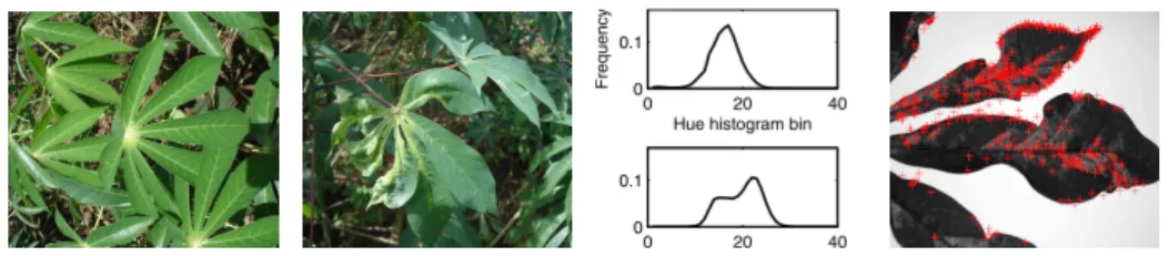
In our experiments we consider the task of diagnosing Cassava Mosaic Disease (CMD) [9]. CMD manifests in crops as decolorization and deformation of the leaves of the plant as shown in Figure 1. Our goal is to diagnose the disease using leaf images as described in previous work on visual cassava disease diagnosis [10]. We extract four sets of features: three sets of color information as normalized histograms (50 bins) of the observed values of Hue, Saturation, and Intensity (HSV) and one set corresponding to local image gradient information, using Scale Invariant Feature Transform (SIFT) descriptors [11] to represent shape features.
Two datasets are considered which were acquired under different conditions: For the lab-cassava dataset images were taken in a lab environment with con-trolled lighting and uniform background. The field-cassava dataset, represents
Fig. 1: Examples of healthy leaves (left), diseased leaves in-situ (middle left), histograms of diseased and healthy leaves (middle right) and examples of SIFT features extracted from a diseased crop image (right).
Data sub-space Dissimilarity measure Parameter setting
H, S and V histograms γ-divergence γ= 1.5
SIFT data (normalized) γ-divergence (CS) γ= 1.0
Table 1: Different dissimilarity measures for different data components images taken in the field with typical background noise including other plants, bare ground, and shadows.
3.2 Experimental set-up
The histograms of Hue, Saturation and Intensity (HSV) and the SIFT features form heterogeneous features of the images. Different dissimilarity measures for the different feature sets are selected based on Table 1. The choice of diver-gences for the HSV histograms’ dissimilarities in the LVQ system is based on previous work [10]. There we explored the advantages of using divergences as dissimilarity measures of distributions or other positive measures as compared to using standard Euclidean measures. The family of γ-divergences is partic-ularly attractive because tuning the parameter γ → 0 results in the popular Kullback-Leibler divergence and forγ= 1, we obtain the Cauchy-Schwarz (CS) divergence. We combined the dissimilarity measures into one global measure as outlined in Section 2.
For the HSV histograms, we selectγ = 1.5, based on empirical observations for a set ofγs (0.5, 1.0, 1.5). The choice ofγ= 1.0 for the SIFT dataset reflects the unique property of the Cauchy-Schwarz divergence, which can be used for non-normalized positive data as well. For these experiments, the matrix Λ was initialized as the identity. The matrix resulting from the training process can be interpreted as a measure for the weight of the dissimilarities in the data sub-spaces for classification.
We performed 4-fold cross-validation repeated for 2 runs each through 100 epochs of the data. We consider a single prototype per class LVQ system. Using more prototypes would have been computationally more expensive but would also have enabled detecting multiple modes in the different classes. However it was not expected that the data would contain multi-modal classes. Training the system follows a batch-gradient descent optimization with a method to control
the step size, presented in [12]. In each step of the procedure prototypes and matrix Ω are updated simultaneously with subsequent normalization.
4
Results
Results in Table 2 are presented as Area Under Curve (AUC) for the test set
Receiver Operating Characteristics (ROC) curves [13]. We compare with first results from previous experiments without combination of the distance measures [10]. The next rows show performance of our method mb-GLVQ with combi-nation of the HSV histograms (second row), and HSV and SIFT subsets (third row).
Feature sets and method Lab-Cassava Field-Cassava HSV without combination 0,86700
-HSV in mb-GLVQ 0,92404 0,97640
HSV+Sift in mb-GLVQ 0,96284 0,97738 Table 2: AUC results for different constellations of the data components We additionally analysed the matrix Λ at the end of training to identify the role of different data sub-spaces for classification. For the lab-cassava HSV dataset, Hue(H) and Intensity(V) histograms play a key role in classification. This result is consistent with previous experiments [10]. When SIFT features are added, we notice a shift in reliance of the classifier to the SIFT features. This probably accounts for the 4 % increase in the AUC performance (92 % to 96 %) shown in Table 2. For the field-cassava HSV dataset, we observe a greater reliance of classification on the Intensity(V) histogram. Adding SIFT features, improves the performance only slightly, probably because obtaining shape and interest point features with a noisy background is not effective. In both cases, the representations of the off-diagonal elements give a similar intuition to the plots of the diagonal of the matrix.
5
Conclusion
The novelty of our method is the integration of different dissimilarity measures using a matrix in an approach similar to [3] in a global GLVQ update scheme. Results from our experiments with cassava leaf data indicate the feasibility of our method. Our method provides superior performance compared to previous work using similar methods on the same datasets. The experiments indicate im-provement in the performance when additional features are added to the example representation.
In future we intend to extend the method to two different application scenar-ios: (i) when different subsets of features represent the same physical entity and (ii) when different dissimilarity measures are applied to the same data. We will also investigate how local distance parameterizations inform the interpretability of the results of the classifier.
References
[1] Eleanor Rosch. Classification of real-world objects: Origins and representations in cogni-tion. Thinking: Readings in Cognitive Science, pages 212–222, 1977.
[2] Dietlind Z¨uhlke, Frank michael Schleif, Tina Geweniger, Sven Haase, and Thomas Vill-mann. Learning vector quantization for heterogeneous structured data. In M. Verleysen, editor,ESANN 2010, pages 271–276. d-side publishing, 2010.
[3] Petra Schneider, Michael Biehl, and Barbara Hammer. Adaptive relevance matrices in learning vector quantization.Neural Comput., 21:3532–3561, December 2009.
[4] Dietlind Z¨uhlke. Vector Quantization based Learning Algorithms for Mixed Data Types and their Application in Cognitive Support Systems for Biomedical Research. PhD thesis, University of Groningen, Netherlands, Johann Bernoulli Institute for Mathematics and Computer Science, Intelligent Systems Group, 2012.
[5] A. Sato and K. Yamada. Generalized learning vector quantization. In Advances in Neural Information Processing Systems 8, pages 423–429, Cambridge, MA, USA, 1996. MIT Press.
[6] Barbara Hammer and Alexander Hasenfuss. Relational neural gas. InKI ’07: Proceedings of the 30th annual German conference on Advances in Artificial Intelligence, pages 190– 204, Berlin, Heidelberg, 2007. Springer-Verlag.
[7] A. K. Qinand and P. N. Suganthan. A novel kernel prototype-based learning algorithm. Pattern Recognition, International Conference on, 4:621–624, 2004.
[8] Tosio Kato. On the adiabatic theorem of quantum mechanics. Journal of the Physical Society of Japan, 5(6):435–439, 1950.
[9] J.R. Aduwo, E. Mwebaze, and J.A. Quinn. Automated vision-based diagnosis of cassava mosaic disease. InIndustrial Conference on Data Mining - Workshops, pages 114–122, 2010.
[10] E. Mwebaze, P. Schneider, F.-M. Schleif, J.R. Aduwo, J.A. Quinn, S. Haase, T. Villmann, and M. Biehl. Divergence based classification in learning vector quantization. Neurocom-puting, 74(9):1429–1435, April 2011.
[11] D.G. Lowe. Distinctive Image Features from Scale-Invariant Keypoints. International Journal of Computer Vision, 60(2):91–110, 2004.
[12] G. Papari, K. Bunte, and M. Biehl. Waypoint averaging and step size control in learning by gradient descent. In MIWOCI 2011, 3rd Mittweida Workshop on Computational Intelligence, Machine Learning Reports, pages 16–26, 2011.