Improving the Multiobjective Evolutionary Algorithm Based on Decomposition with New Penalty Schemes

(will be inserted by the editor)

Improving the Multiobjective Evolutionary Algorithm Based on

Decomposition with New Penalty Schemes

Shengxiang Yang _· Shouyong Jiang _· Yong Jiang

Received: September 23, 2015; Revised: December 9, 2015; Accepted: January 26, 2016

Abstract It has been increasingly reported that the multi-objective optimization evolutionary algorithm based on de-composition (MOEA/D) is promising for handling multiob-jective optimization problems (MOPs). MOEA/D employs scalarizing functions to convert an MOP into a number of single-objective subproblems. Among them, penalty bound-ary intersection (PBI) is one of the most popular decom-position approaches and has been widely adopted for deal-ing with MOPs. However, the original PBI uses a constant penalty value for all subproblems and has difficulties in achieving a good distribution and coverage of the Pareto front for some problems. In this paper, we investigate the influence of the penalty factor on PBI, and suggest two new penalty schemes, i.e., adaptive penalty scheme (APS) and subproblem-based penalty scheme (SPS), to enhance the spread of Pareto optimal solutions. The new penalty schemes are examined on several complex MOPs, show-ing that PBI with the use of them is able to provide a bet-ter approximation of the Pareto front than the original one. The SPS is further integrated into two recently developed MOEA/D variants to help balance the population diversity and convergence. Experimental results show that it can sig-nificantly enhance the algorithm’s performance.

Shengxiang Yang

School of Mathematics and Statistics, Nanjing University of Informa-tion Science and Technology, Nanjing 210044, China; and Centre for Computational Intelligence (CCI), School of Computer Science and In-formatics, De Montfort University, Leicester LE1 9BH, U.K. E-mail: [email protected]

Shouyong Jiang

Centre for Computational Intelligence (CCI), School of Computer Sci-ence and Informatics, De Montfort University, Leicester LE1 9BH, U.K. E-mail: [email protected]

Yong Jiang

School of Mathematics and Statistics, Nanjing University of Infor-mation Science and Technology, Nanjing 210044, China. E-mail: [email protected]

Keywords Multiobjective evolutionary algorithm· decom-position·penalty boundary intersection·adaptive penalty scheme·subproblem-based penalty scheme

1 Introduction

Many real-world optimization problems, such as water re-source management (Reed et al., 2013), design optimization (Deb and Jain, 2014; Yang and Deb, 2013), and land use management (Chikumbo, 2012; Masoomi et al., 2013), of-ten have multiple objectives that conflict with each other. Without lose of generality, these kinds of multiobjective op-timization problems (MOPs) can be described as follows:

minF₍x_{) = (f}1(x), ..., fM(x))T s.t.    hi(x_{) = 0, i= 1, ..., nh} gi(x_{)≥0, i= 1, ..., ng} x_∈Ωx (1)

whereΩx ⊆ Rn _{is the decision space, nh andng are the} number of equalities and inequalities, respectively,M is the number of objectives, andF₍x_):Ωx→RM_{is the objective} function vector of the solutionx_{. Due to the nature of} con-flict among objectives, there does not exist a single optimal solution that can minimize all the objectives simultaneously. As a consequence, the optimization goal of MOPs is to ob-tain a set of solutions with a good trade-off among the objec-tives. The set of trade-off solutions is known as the Pareto-optimal set (POS), and its image in the objective space is called the Pareto-optimal front (POF).

Multiobjective evolutionary algorithms (MOEAs) are an important class of methods devoted to solving MOPs. They employ a population of candidate members and evolve them collaboratively, resulting in a number of candidate solutions in a single run, without the use of any gradient information of MOPs. These characteristics make MOEAs very suitable

for handling MOPs. After several decades of effort to the field of evolutionary computation, a huge number of MOEAs are available to date. They can be classified into three main groups: Pareto-based approaches (Deb et al., 2002; Knowles and Corne, 1999; Zitzler et al., 2002; Deb and Jain, 2014), indicator-based approaches (Bader and Zitzler, 2011; Beume et al., 2007; Ishibuchi et al., 2010; Zitzler and Kunzli, 2004), and decomposition-based approaches (Zhang and Li, 2007; Li and Zhang, 2009; Asafuddoula et al., 2015). The MOEA based on decomposition (MOEA/D) is the most well-known representative of decomposition-based approaches. It uses scalarizing functions or decomposition approaches to de-compose an MOP into a number of single-objective sub-problems and optimize them in a co-evolutionary manner. In MOEA/D, weight vectors or search directions involved in the scalarizing functions implicitly manage population di-versity, and the concept of neighbourhood is introduced to co-evolve solutions of neighbouring subproblems. This way, MOEA/D can quickly approximate the Pareto front and pro-vide a set of diverse solutions. Recently, various versions of MOEA/D have been proposed in the literature (Zhang and Li, 2007; Li and Zhang, 2009; Asafuddoula et al., 2015; Li et al., 2015a; Jiang and Yang, 2015), and the idea of decom-position has been exploited in a number of studies (Deb and Jain, 2014; Li et al., 2014b,c, 2015a,b; Liu et al., 2014; Yuan et al., 2015).

In MOEA/D, there are three widely-used scalarizing functions, i.e., weighted sum, weighted Tchebycheff, and penalty boundary intersection (PBI), to aggregateM differ-ent objectives (Zhang and Li, 2007). Compared with PBI, the weighted sum and weighted Tchebycheff are easier to implement and less computationally expensive. A recent study (Ishibuchi et al., 2013) reported that the weighted sum shows better search performance than the weighted Tcheby-cheff in many-objective problems. However, the weighted sum is not effective to approximate problems with the entire concave Pareto front (Zhang and Li, 2007). The weighted Tchebycheff approach has received intensive research inter-est due to its ability to approximate both convex and concave POFs. Despite its great success for solving standard bench-mark problems like ZDT (Zitzler et al., 2000) or DTLZ (Deb et al, 2005), some recent investigations have revealed that this approach has difficulties in uniformly distributing solu-tions on boundary regions of the POF for complex problems (Qi et al., 2014; Jiang and Yang, 2015). On the other hand, the PBI approach gains a firm foothold in MOEA/D be-cause it can provide a more uniform distribution of POF than the weighted Tchebycheff for three- and higher-dimensional problems (Li et al., 2015a; Zhang and Li, 2007; Deb and Jain, 2014; Gomez and Coello Coello, 2015).

It is not very surprising that PBI has obtained great suc-cess for multiobjective and many-objective problems since its introduction. Probably due to the lack of complicated

POF characteristics in the well-known ZDT (Zitzler et al., 2000), DTLZ (Deb et al, 2005) and WFG (Huband et al., 2006) test suites in the field of multiobjective optimization, PBI has been rarely or even not deeply examined on prob-lems with complicated POFs. However, real-world MOPs often have irregular POF geometries (Deb et al., 2000; Osy-cza and Kundu, 1995; Wang et al., 2013), where the shape can be extremely convex and/or concave. Note that, there are also other kinds of irregularities, such as degenerate and disconnected POFs (Cheng et al., 2015; Jain and Deb, 2013; Giagkiozis et al., 2014), which may be harder than extremely-shaped POFs. As a starting point, we just con-sider irregular extremely-shaped POFs in this paper. While it has been repeatedly reported that PBI works well on regu-lar problems, one may wonder whether PBI can continue its success on the real-life or artificial problems with compli-cated POFs. If not, the applicability of PBI (Zhang and Li, 2007; Al Moubayed et al., 2013; Pavelski et al., 2014; Jia et al., 2011) and its extension to many-objective optimiza-tion (Cheng et al., 2016; Deb and Jain, 2014; Gomez and Coello Coello, 2015; Li et al., 2014a, 2015a; Mohammadi et al., 2014; Yuan et al., 2014; Mendez and Coello Coello, 2015; Gomez and Coello Coello, 2015), which has become a recent hot topic, could be questioned.

The performance of PBI is largely determined by its penalty factor, which controls the balance between conver-gence and diversity. A small penalty favours converconver-gence whereas a large one stresses diversity. The penalty value was commonly set to 5.0 in most studies, e.g., (Deb and Jain, 2014; Zhang and Li, 2007; Li et al., 2015a). However, in (Ishibuchi et al., 2015), PBI with a penalty value of 0.1 was reported to outperform that with a penalty value of 5.0 on multiobjective knapsack problems. This means, the opti-mal value for the penalty factor may vary dramatically from problems to problems. Also, in the case of small penalty val-ues, if the distance from the obtained ideal point to boundary solutions is significantly larger than that to intermediate so-lutions, boundary solutions are likely to be abandoned dur-ing the search because of the poor convergence measured by the distance. In the case of large penalty values, due to overemphasis of diversity, population individuals need more computational resources to explore the search space before converging to the POF. Besides, Sato (2014) argued that if the obtained ideal point is far from the true ideal point (probably due to the loss of boundary solutions), PBI will face difficulties to approximate the entire POF. Therefore, the author suggested an inverted version of PBI to ease this problem. Nevertheless, the inverted PBI fails to consider the influence of the penalty factor, and may still get stuck into the difficulty of tuning this parameter.

In this paper, we first study the influence of the penalty factor on the search performance of PBI, fol-lowed by suggesting two new penalty schemes, i.e.,

adap-tive penalty scheme (APS) and subproblem-based penalty scheme (SPS). APS adaptively assigns all subproblems the same penalty value by taking into consideration different re-quirements at different search stages, whereas SPS specifies distinct penalty values for different subproblems at an at-tempt to enhance the spread of POF. These schemes are ex-amined on several complex problems and experimental re-sults demonstrate their promise for improving PBI’s perfor-mance. Besides, SPS is further integrated into some newly-developed MOEA/D variants, showing that it significantly improves the performance of these algorithms.

The rest of this paper is outlined as follows. Section 2 briefly reviews related work on MOEA/D. Section 3 first presents an investigation into the influence of the penalty factor on PBI and then introduces the two penalty schemes proposed for PBI. In Section 4, the experimental study is conducted on the proposed penalty schemes. Section 5 con-cludes this paper and discusses some future work.

2 Related Work 2.1 The PBI Approach

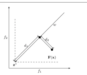
Decomposition approaches play a key role in converting an MOP into a number of scalar optimization subprob-lems in decomposition-based MOEAs. There are three pop-ular decomposition approaches, such as the weighted sum, weighted Tchebycheff and PBI. The weighted sum approach favours convex problems and fails to approximate problems with a concave POF, whereas the weighted Tchebycheff ap-proach can handle both convex and concave problems. The PBI approach has its advantages in obtaining a good dis-tribution of solutions in the objective space (Zhang and Li, 2007) and handling many-objective problems (Deb and Jain, 2014; Ishibuchi et al., 2015), but its performance is very sen-sitive to the setting of the penalty factor (Ishibuchi et al., 2015). The scalar optimization problem of PBI is defined as follows: mingpbi_(x|w,z∗_{) =d} 1+θd2 s.t.x_∈Ωx (2) where d1= k(F₍x₎₋z∗₎T_wk kw_k (3) d2=kF(x)−(z∗+d1 w kw_k)k (4)

Ωxis the search space andz∗ _{= (z}∗

1,· · · , z_M∗ )is the ideal

point in the objective space for which theith component can be computed byz∗

i = min

x∈Ωx

fi(x_{), andθ is a user-defined} penalty factor.d1andd2are the length of the projection of

f2 f1 z∗ F(x) w d1 d2

Fig. 1 Illustration of PBI.

vector (F₍x₎₋z∗_{) on the weight vectorwand the}

perpen-dicular distance fromF₍x_)tow_{, respectively. Fig. 1 offers} a brief illustration of the PBI approach. It is not difficult to see thatθtakes the responsibility for balancing convergence (measured byd1) and diversity (measured byd2), and the

PBI approach drives the search toward the obtained ideal pointz∗_{by minimizingg}pbi_.

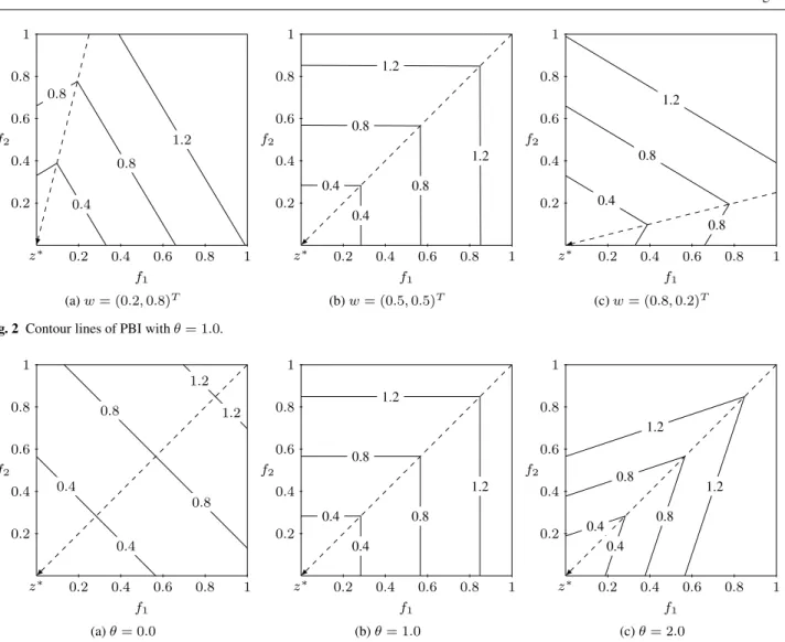
Figure 2 shows the contour lines of PBI withθ= 1.0on three different two-dimensional weight vectors, where dif-ferent weight vectors specify distinct promising search re-gions in the objective space. This means each weight vector can direct the search toward its preferred POF segment, and by employing a number of well-spread weight vectors, the whole POF can be approximated. To illustrate the influence of the penalty factorθ, we also plot the contour lines of PBI onw _{= (0.5,0.5)}T _{forθ= 0.0, 1.0 and 2.0 in Fig. 3. The} figure indicates that different values ofθ lead to different search behaviours and a large value ofθ narrows efficient search regions and promotes diversity.

2.2 MOEA/D Algorithm

MOEA/D employs a set of predefined weight vectors that uniformly partition the entire objective space to specify a number of search directions, and defines a single-objective problem or a multiobjective subproblem by decomposition approaches for each search direction. For each search direc-tion, MOEA/D also specifiesT closest neighbours before-hand, which helps to efficiently solve the associated single-objective problem in a collaborative manner. During the course of search, mating selection and replacement are con-sidered among solutions associated with theTneighbouring search directions. MOEA/D is a steady-state algorithm and updates solutions one by one, so it approximates the true POF quickly. Algorithm 1 presents a brief description of the original MOEA/D with the PBI (Zhang and Li, 2007). For more details, the interested readers are referred to (Zhang and Li, 2007).

f2 f1 z∗ 0.4 0.8 0.8 1.2 0.2 0.4 0.6 0.8 1 0.2 0.4 0.6 0.8 1 f2 f1 z∗ 0.4 0.4 0.8 0.8 1.2 1.2 0.2 0.4 0.6 0.8 1 0.2 0.4 0.6 0.8 1 f2 f1 z∗ 0.4 0.8 0.8 1.2 0.2 0.4 0.6 0.8 1 0.2 0.4 0.6 0.8 1 (a)w= (0.2,0.8)T _{(b)w= (0.5,0.5)}T _{(c)w= (0.8,0.2)}T

Fig. 2 Contour lines of PBI withθ= 1.0.

f2 f1 z∗ 0.4 0.4 0.8 0.8 1.2 1.2 0.2 0.4 0.6 0.8 1 0.2 0.4 0.6 0.8 1 f2 f1 z∗ 0.4 0.4 0.8 0.8 1.2 1.2 0.2 0.4 0.6 0.8 1 0.2 0.4 0.6 0.8 1 f2 f1 z∗ 0.4 0.4 0.8 0.8 1.2 1.2 0.2 0.4 0.6 0.8 1 0.2 0.4 0.6 0.8 1 (a)θ= 0.0 (b)θ= 1.0 (c)θ= 2.0

Fig. 3 Contour lines of PBI withw= (0.5,0.5)T_.

Algorithm 1MOEA/D-PBI

1: Input:

– M axI teration: the stopping criterion

– N: the number of subproblems considered in MOEA/D – T: the neighbourhood size

2: Output: approximated Pareto-optimal set

3: Initialization:Generate a uniform spread ofN weight vectors:

w1

, . . . , wN _{and then compute theT closest weight vectors to}

each weight vector by the Euclidean distance. For each i =

1, . . . , N, setB(i) ={i1, . . . , iT}wherewi1_{, . . . , w}iT _{are the}

Tclosest weight vectors towi

4: Generate an initial populationP = {x1

, . . . , xN_{}by uniformly}

randomly sampling from the decision space 5: whilegen:= 1toM axI terationdo 6: fori:= 1toNdo

7: Randomly select two indexesr1andr2fromB(i) 8: Apply genetic operators on individualsr1,r2to produce a

new solutiony

9: If y is better than any individual xj _{in B(i) (i.e.,}

gpbi_(y

|wj_{, z}∗_{) ≤ g}pbi_(xj_|wj_{, z}∗_{)), thenx}j _{is replaced}

byy

10: end for 11: end while 12: OutputP

3 Proposed Penalty Schemes for MOEA/D with PBI 3.1 Influence of the Penalty Factor

As mentioned earlier,θ is a key factor for balancing con-vergence and diversity in PBI. A small value ofθ favours convergence whereas a large one is beneficial for diversity. Figures 4 and 5 show the influence of two differentθvalues on convergence and diversity, where the bold curve is the true POF and points A to G are scattered POF points.

In Fig. 4, θ is set to 1.0, and its influence is illus-trated by two adjacent boundary weight vectors, i.e.,w1 =

(0.1,0.9)T _andw

2 = (0.2,0.8)T. Intuitively, B and C are

ideal optimal points for subproblems associated with w1

andw2, respectively. However, the solutionB of the

sub-problem associated withw1 will be replaced withC since

gpbi_(C|w

1, z∗) = 0.60 is smaller than gpbi(B|w1, z∗) =

0.75. This means, due to insufficient penalty, POF points far away from the obtained ideal pointz∗_{are replaced by those}

f2 f1 z∗ w1 w2 0.75 0.60 A B C D E F G 0.2 0.4 0.6 0.8 1 0.2 0.4 0.6 0.8 1

Fig. 4 Illustration of insufficient penalty for weight vectors where

w1= (0.1,0.9)T_{,w2= (0.2,0.8)}T _{andθ= 1.0is used in PBI.}

f2 f1 z∗ w1 w2 0.80 0.8 I J H A B C D E F G 0.2 0.4 0.6 0.8 1 0.2 0.4 0.6 0.8 1

Fig. 5 Illustration of excessive penalty for weight vectors wherew1= (0.5,0.5)T_{,w2= (0.4,0.6)}T _{andθ= 5.0is used in PBI.}

worse, for extremely-convex problems that have a sharp peak and long tail (Jiang and Yang, 2015), the above im-pact is more vital, and boundary points on the POF cannot be approximated so as to decrease the spread of the POF.

In Fig. 5,w1= (0.5,0.5)T andw2= (0.4,0.6)T are two

adjacent intermediate weight vectors, and a large value of θ = 5.0 is used in PBI. For w1, PBI is expected to drive

the search toward the POF segment between D and E. At the early stage of search, the subproblems associated with w1 andw2 find their best solutionH andJ, respectively.

Clearly,J is much closer thanH to the expected POF seg-ment. But, for the subproblem associated withw1, its

cur-rent solutionHwill not be replaced byJ asJgives a larger gpbi_{thanH. This indicates, due to excessive penalty,} solu-tions close to weight vectors but far away from the POF may be preferred over those close to the POF but far away from the weight vectors. This inevitably spoils PBI’s convergence performance and slows down the whole search process.

3.2 Adaptive Penalty Scheme (APS)

Facing the above-mentioned difficulties, one may naturally turn to adaptively adjusting the magnitude of penalty at dif-ferent search stages. At the early stage, the main optimiza-tion goal is to drive the search toward the POF as fast as pos-sible, so a small value ofθis helpful for fast convergence. In contrast, at the late stage, the obtained solutions are required to be diverse and spread so that they will not miss any part of the entire POF. Thus, the late search stage focuses on di-versity, and a large value ofθ is expected to diversify the solutions.

In this paper, we propose to use the APS to balance the population convergence and diversity at different stages, which is described as follows:

θ=θmin+ (θmax−θmin) t

maxIteration (5)

wheretis the iteration counter,maxIterationis the maxi-mum number of iterations,θminandθmaxare the lower and upper bounds ofθ, respectively. Here, these two parameters are suggested to beθmin = 1.0 andθmax = 10.0, which ensuresθ = 5recommended by Zhang and Li (2007) is in the interval[θmin, θmax].

Note that, the APS used in this paper is linear and serves as an example for validating the promise of this kind of method to enhance PBI. In principle, any proper nonlinear APS can fulfil this purpose.

3.3 Subproblem-based Penalty Scheme (SPS)

Another alternative way to reduce the drawback of PBI is to specify independently a penalty value for each subproblem. As explained in Section 3.1, for convex problems, boundary solutions are much further than intermediate solutions from the obtained ideal point, so boundary subproblems should be given strict penalties on diversity measure to avoid unrea-sonable replacements. For concave problems, although there is no much difference between boundary solutions and inter-mediate solutions in terms of their distance to the obtained ideal point, strict penalty on boundary solutions might also help maintain diversity.

The idea behind the SPS is simple, but it is not easy to assignNdifferent penalty values forNsubproblems. Also, such assignments may be computationally expensive. Hav-ing realized that each subproblem is mainly determined by its weight vector and there are distinct differences between boundary and intermediate weight vectors, we elaborate the following SPS for PBI:

θi=eαβi ₍₆₎ βi= max 1≤j≤Mw j i −_1≤min j≤Mw j i (7)

whereθi denotes the penalty value for a weight vectorwi, andβi is the difference between the maximum component and the minimum component inwi. Since PM

j=1w

j i = 1 andw_ij ≥ 0 for any1 ≤ j ≤ M,βi lies in [0,1]. For in-termediate weight vectors, i.e., all components are almost identical,βi is close to 0, while for boundary weight vec-tors, particularly those lying on theM coordinate axes,βi has a value of one.αis a non-negative value controlling the magnitude of penalty andα = 4.0is recommended in this paper based on some preliminary studies. The exponential formulation used here ensures that the penalty value is al-ways positive.

4 Experimental Study 4.1 Experimental Settings

To examine the effectiveness of our proposed schemes, we use six complex problems with irregular Pareto fronts in-stead of some well-known test suites such as ZDT (Zitzler et al., 2000) or DTLZ (Deb et al, 2005) for empirical com-parison. Some of them have been tested in (Jiang and Yang, 2015) and (Deb and Jain, 2014), showing that the original MOEA/D faces difficulties in solving these kinds of prob-lems due to their complex characteristics. The detailed de-scription of these problems is presented in Table 1.

The proposed two penalty schemes, i.e., APS and SPS, are compared with the original PBI. MOEA/D1 _{with these} different penalty schemes was implemented in C++.θin the canonical PBI was set to 5.0, and this kind of setting has been widely adopted in the literature (Zhang and Li, 2007; Deb and Jain, 2014; Li et al., 2015a). The neighbourhood sizeT was set to 20. The crossover probability was set to pc= 1.0and its distribution index wasηc= 20. The muta-tion probability was set topm = 1/n, wherenis the num-ber of variables, and its distributionηm = 20. We set the population sizeNto 100 for bi-objective problems and 190 for three-objective problems. The stopping criterion was set to 100 generations. For all the test problems, the MOEA/D variants were executed 30 independent runs.

4.2 Performance Metrics

In the experiments, we use three performance measures, which are described below.

4.2.1 Maximum Spread (MS)

The MS, first introduced by Zitzler et al. (Zitzler et al., 2000), measures to what extent the extreme members in an approximated Pareto front P OF∗

has been reached. Goh 1 _{Source code available from http://dces.essex.ac.uk/staff/qzhang/.}

and Tan (Goh and Tan, 2007) proposed a modified version of MS by taking into account the proximity ofP OF∗

to-wards the true Pareto frontP OF:

MS′= v u u t1 M M X k=1 " min[POFk, POF∗ k]−max[POFk, POF ∗ k] P OF∗ k −P OFk∗ #2 (8)

whereP OFk andP OFk are the maximum and minimum of thekth objective inP OF, respectively; Similarly,P OF∗

k andP OF∗

k are the maximum and minimum of thekth objec-tive inP OF∗

, respectively. A large value ofM S′

indicates a good spread ofP OF∗_{, andM S}′_{will have a value of one}

whenP OF∗_{covers the wholeP OF.}

4.2.2 Inverted Generational Distance (IGD)

The IGD (Zitzler et al., 2003) is an effective performance in-dicator since it can provide reliable information on both the diversity and convergence of obtained solutions. LetP F be a set of solutions uniformly sampled from the true POF, and P F∗ _{be the approximated solutions in the objective space,}

the IGD metric measures the gap betweenP F∗ _{andP F,}

which is calculated as follows:

IGD(P F∗_{, P F) =} P p∈P Fd(p, P F ∗₎ |P F| (9) whered(p, P F∗₎

is the distance between the memberpof P F and the nearest member of P F∗_{. In this paper, 500}

points uniformly sampled from the true POF are used as the reference set for IGD, which can be done by generating a large volume of points and then pruning them to the desir-able size by thekth nearest neighbour method proposed in the strength Pareto evolutionary algorithm 2 (SPEA2) (Zit-zler et al., 2002).

4.2.3 Hypervolume (HV)

HV (Zitzler and Thiele, 1999) measures the size of the ob-jective space dominated by the approximated solutions S and bounded by a reference pointR= (R1, . . . , RM)T that

is dominated by all points on the POF, and is computed by:

HV(S) =Leb( ∪

x∈S[f1(x), R1]× · · · ×[fM(x), RM]) (10) whereLeb(A)is the Lebesgue measure of a setA. In our experiments,Ris set to(1.2,1.2)T _{and(1.2,1.2,1.2)}T _for bi- and three-objective test instances, respectively.

Table 1 Test Instances

Instance Description Domain Number of Variables Notes

F1 f1(x) = (1 +g(x))x1 f2(x) = (1 +g(x))(1−√x1)3 g(x) = 2 sin(0.5πx1)(n−1 + n P i=2 (y2 i −cos(2πyi))) whereyi=2:n=xi−sin(0.5πxi) POF:f2= (1−√f1)3 POS:xi= sin(0.5πxi), i= 2, . . . , n [0,1]n ₂₀ Uni-modal Convex F2 f1(x) = (1 +g(x))x1 f2(x) = (1 +g(x))√1−x15 g(x) = 2 sin(0.5πx1)(n−1 + Pn i=2 (y2 i −cos(2πyi))) whereyi=2:n=xi−sin(0.5πxi) POF:f2=p1−f15 POS:xi= sin(0.5πxi), i= 2, . . . , n [0,1]n ₂₀ Uni-modal Convex F3 f1(x) = (1 +g(x))x1 f2(x) = 1 2(1 +g(x))(1−x 0.1 1 + (1−√x1) 2 cos2 (3πx1)) g(x) = 2 sin(0.5πx1)(n₋1 + n P i=2 (y2 i −cos(2πyi))) whereyi=2:n=xi−sin(0.5πxi) POF:f2= 1 2(1−f 0.1 1 + (1− √ f1)2cos2(3πf1)) POS:xi= sin(0.5πxi), i= 2, . . . , n [0,1]n ₂₀ Multi-modal Disconnected F4 f1(x) = (1 +g(x))(x1+ 0.05 sin(6πx1))2 f2(x) = (1 +g(x))(1−x1+ 0.05 sin(6πx1))2 g(x) = 2 sin(0.5πx1)(n−1 + n P i=2 (y2 i −cos(2πyi))) whereyi=2:n=xi−sin(0.5πxi) POF:f0.5 1 +f 0.5 2 = 1 + 0.1 sin(3π(f 0.5 1 −f 0.5 2 + 1)) POS:xi= sin(0.5πxi), i= 2, . . . , n [0,1]n ₂₀ Multi-modal mixed F5 f1(x) = (1 +g(x))(x1+ 0.05 sin(6πx1))0.2 f2(x) = (1 +g(x))(1−x1+ 0.05 sin(6πx1))10 g(x) = 2 sin(0.5πx1)(n−1 + n P i=2 (y2 i −cos(2πyi))) whereyi=2:n=xi−sin(0.5πxi) POF:f5 1+f 0.1 2 = 1 + 0.1 sin(3π(f 5 1−f 0.1 2 + 1)) POS:xi= sin(0.5πxi), i= 2, . . . , n [0,1]n ₂₀ Multi-modal mixed F6 f1(x) = ((1 +g(x)) cos(0.5πx1) cos(0.5πx2))4 f2(x) = ((1 +g(x)) cos(0.5πx1) sin(0.5πx2))4 f3(x) = ((1 +g(x)) sin(0.5πx1))2 g(x) = n P i=3 (xi−0.5)2 POF:√f1+√f2+f3= 1 POS:xi= 0.5, i= 3, . . . , n [0,1]n ₂₀ Uni-modal Convex 4.3 Experimental Results

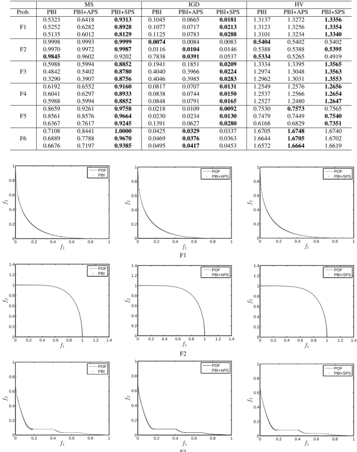
Table 2 records MS, IGD and HV values obtained by PBI, PBI+APS and PBI+SPS for F1 to F6, where the best value for each problem and each performance metric is marked in bold face. From Table 2, it can be seen that both the pro-posed penalty schemes are helpful for improving the per-formance of PBI. Specifically, on the MS metric, the use of APS and SPS can provide a better coverage of POF for most of the problems compared with the original PBI, and SPS improves the coverage much more than APS. The IGD metric suggests that APS and SPS can give better distribu-tion of obtained points along the POF for all the problems except F2. Besides, the HV metric further indicates the ef-fectiveness of APS and SPS for most of the problems, and

SPS significantly improves the performance of PBI except on F2. Note that, PBI with APS or SPS does not offer notice-able improvement on the MS, IGD and HV metrics for F2. This may be because F2 is a concave problem and there is no considerable difference between boundary solutions and intermediate solutions in terms of their distance to the ob-tained ideal point. This negligible difference implies that all the decomposed subproblems have similar convergence per-formance in PBI. In this case, diversity is the only influenc-ing factor, and thus a fixed and identical penalty value can help all the problems reach the same level of balance be-tween diversity and convergence, which may be suitable for solving such kind of problem. Nevertheless, the use of APS and SPS does not degrade PBI’s performance in this case.

Table 2 Best, mean and worst performance measure values obtained by three penalty schemes on six problems

MS IGD HV

Prob. PBI PBI+APS PBI+SPS PBI PBI+APS PBI+SPS PBI PBI+APS PBI+SPS

F1 0.5323 0.6418 0.9313 0.1045 0.0665 0.0181 1.3137 1.3272 1.3356 0.5252 0.6282 0.8928 0.1077 0.0717 0.0213 1.3123 1.3256 1.3354 0.5135 0.6012 0.8129 0.1125 0.0783 0.0288 1.3101 1.3234 1.3340 F2 0.9998 0.9993 0.9999 0.0074 0.0084 0.0083 0.5404 0.5402 0.5402 0.9970 0.9972 0.9987 0.0116 0.0104 0.0146 0.5388 0.5388 0.5395 0.9845 0.9602 0.9202 0.7838 0.0391 0.0537 0.5334 0.5265 0.4919 F3 0.5988 0.5994 0.8852 0.1941 0.1851 0.0209 1.3334 1.3395 1.3565 0.4842 0.5402 0.8780 0.4040 0.3966 0.0224 1.2974 1.3048 1.3563 0.3290 0.3907 0.8756 0.4046 0.3985 0.0283 1.2962 1.3031 1.3553 F4 0.6192 0.6552 0.9160 0.0817 0.0707 0.0131 1.2549 1.2576 1.2656 0.6041 0.6297 0.8933 0.0838 0.0744 0.0150 1.2537 1.2566 1.2654 0.5988 0.5994 0.8852 0.0848 0.0791 0.0165 1.2527 1.2480 1.2647 F5 0.8659 0.9261 0.9758 0.0218 0.0109 0.0092 0.7530 0.7573 0.7565 0.8561 0.8576 0.9664 0.0230 0.0234 0.0130 0.7479 0.7449 0.7540 0.6367 0.7617 0.9245 0.1391 0.0627 0.0280 0.6168 0.6829 0.7351 F6 0.7108 0.8441 1.0000 0.0425 0.0329 0.0337 1.6705 1.6748 1.6740 0.6889 0.7788 0.9670 0.0469 0.0376 0.0363 1.6644 1.6705 1.6702 0.6676 0.7197 0.9385 0.0495 0.0417 0.0453 1.6572 1.6664 1.6619 0 0.2 0.4 0.6 0.8 1 0 0.2 0.4 0.6 0.8 1 f1 f2 POF PBI 0 0.2 0.4 0.6 0.8 1 0 0.2 0.4 0.6 0.8 1 f1 f2 POF PBI+APS 0 0.2 0.4 0.6 0.8 1 0 0.2 0.4 0.6 0.8 1 f1 f2 POF PBI+SPS F1 0 0.2 0.4 0.6 0.8 1 1.2 1.4 0 0.2 0.4 0.6 0.8 1 1.2 1.4 f1 f2 POF PBI 0 0.2 0.4 0.6 0.8 1 1.2 1.4 0 0.2 0.4 0.6 0.8 1 1.2 1.4 f1 f2 POF PBI+APS 0 0.2 0.4 0.6 0.8 1 1.2 1.4 0 0.2 0.4 0.6 0.8 1 1.2 1.4 f1 f2 POF PBI+SPS F2 0 0.2 0.4 0.6 0.8 1 0 0.2 0.4 0.6 0.8 1 f1 f2 POF PBI 0 0.2 0.4 0.6 0.8 1 0 0.2 0.4 0.6 0.8 1 f1 f2 POF PBI+APS 0 0.2 0.4 0.6 0.8 1 0 0.2 0.4 0.6 0.8 1 f1 f2 POF PBI+SPS F3 Fig. 6 Approximated POFs with the lowest IGD values among 30 runs on F1-F3.

0 0.2 0.4 0.6 0.8 1 0 0.2 0.4 0.6 0.8 1 f1 f2 POF PBI 0 0.2 0.4 0.6 0.8 1 0 0.2 0.4 0.6 0.8 1 f1 f2 POF PBI+APS 0 0.2 0.4 0.6 0.8 1 0 0.2 0.4 0.6 0.8 1 f1 f2 POF PBI+SPS F4 0 0.2 0.4 0.6 0.8 1 1.2 0 0.2 0.4 0.6 0.8 1 1.2 f1 f2 POF PBI 0 0.2 0.4 0.6 0.8 1 1.2 0 0.2 0.4 0.6 0.8 1 1.2 f1 f2 POF PBI+APS 0 0.2 0.4 0.6 0.8 1 1.2 0 0.2 0.4 0.6 0.8 1 1.2 f1 f2 POF PBI+SPS F5 0 0.5 1 0 0.5 1 0 0.5 1 f1 f2 f3 POF PBI 0 0.5 1 0 0.5 1 0 0.5 1 f1 f2 f3 POF PBI+APS 0 0.5 1 0 0.5 1 0 0.5 1 1.5 f1 f2 f3 POF PBI+SPS F6 Fig. 7 Approximated POFs with the lowest IGD values among 30 runs on F4-F6.

For a better understanding of the improvement provided by our proposed penalty schemes, we also present graphical plots of approximated POFs for the six problems in Figs. 6 and 7. It can be clearly observed from the figures that, both PBI+APS and PBI+SPS help to find more boundary points than the original PBI for F1, F3, F4 and F6 so as to stretch out their approximated POFs, and PBI+SPS performs much better than PBI+APS in doing this. For the overall concave F2 and F5 problems, three PBI variants show nearly similar distribution of obtained solutions, although PBI+SPS seems to find more boundary points than PBI and PBI+APS for F5.

It is understandable that PBI+SPS performs the best in most cases. This can be attributed to the feature that PBI+SPS imposes strict penalty on boundary subproblems so that it is capable of finding boundary points.

4.4 Integration into MOEA/D Variants

The previous subsection clearly shows the effectiveness of the two proposed penalty schemes, and SPS generally per-forms better than APS. In this subsection, SPS is inte-grated into two newly-proposed variants of MOEA/D, i.e., MOEA/D-ACD (Wang et al., 2015) and MOEA/D-STM (Li et al., 2014c), to examine whether SPS can help improve the performance of PBI-based algorithms.

4.4.1 Integration into MOEA/D-ACD

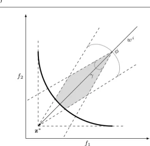
MOEA/D-ACD uses constrained decomposition approaches to convert an MOP into a number of single-objective sub-problems. The basic idea behind it is to add constraints to the decomposed subproblems to shrink improvement regions. For thewi _{search direction in MOEA/D, the resulting}

con-f2 f1 z∗ φ γ wi

Fig. 8 Illustration of the improvement region (marked in grey) for the constrained PBI approach.

strained subproblemiis defined as follows: ming(x_|wi_,z∗₎

s.t.hwi_,F₍x₎₋z∗_{i ≤} φ

2

x∈Ωx

(11)

whereg(·)is the scalarizing objective function defined by a decomposition approach,hwi_,F₍x₎₋z∗_{iis the acute angle}

betweenwi_andF₍x₎₋z∗_{, andφis a parameter controlling} the size of improvement regions. The value ofφis different for different subproblems. Fig. 8 illustrates the improvement region of the constrained PBI approach for subproblemi.

It can be clearly observed from Fig. 8 that the enclosed improvement region for the constrained PBI is mainly con-trolled by two acute angles, i.e., φ andγ, whereγ is de-termined by the penalty factor θ. A constant θ value in MOEA/D-ACD means all subproblems have the same γ, and the improvement regions may be still too large for some subproblems although the constrained decomposition ap-proach is used. As a result, a new solution can replace sev-eral different old but well-distributed solutions, thus impair-ing the population diversity. In contrast, if each subproblem is assigned a different and properθvalue, the improvement regions will be well controlled, which may help maintain the balance between the population diversity and convergence.

It should be noted that our proposed SPS and the con-strained approach in MOEA/D-ACD are similar in some sense because both are based on the assumption that each subproblem should separately maintain an appropriately dif-ferent balance between diversity and convergence. When SPS is integrated into MOEA/D-ACD, it is expected that SPS can help improve the performance of MOEA/D-ACD. For this reason, we compare the integrated MOEA/D with MOEA/D-ACD on our previously used test problems. For notation convenience, MOEA/D-ACD is denoted as “ACD” and MOEA/D-ACD with SPS as “ACD+SPS” later on.

Table 3 Best, mean and worst performance measure values obtained by ACD and ACD+SPS

MS IGD HV

Prob. ACD ACD+SPS ACD ACD+SPS ACD ACD+SPS

F1 0.8257 0.9623 0.0270 0.0196 1.3340 1.3351 0.7538 0.8653 0.0390 0.0228 1.3318 1.3337 0.6466 0.7405 0.0640 0.0440 1.3267 1.3311 F2 0.9999 0.9996 0.0164 0.0205 0.5397 0.5383 0.9988 0.9982 0.0239 0.0320 0.5363 0.5342 0.9914 0.9936 0.0399 0.0371 0.5294 0.5280 F3 0.8343 0.8816 0.0278 0.0190 1.3531 1.3559 0.7431 0.8600 0.0410 0.0218 1.3509 1.3552 0.5322 0.6116 0.1763 0.1738 1.3389 1.3435 F4 0.9160 0.9184 0.0147 0.0143 1.2630 1.2643 0.8600 0.8930 0.0208 0.0166 1.2613 1.2626 0.8020 0.8723 0.0274 0.0200 1.2584 1.2606 F5 0.9865 0.9889 0.0085 0.0105 0.7548 0.7578 0.9210 0.9278 0.0173 0.0137 0.7497 0.7502 0.8659 0.8937 0.0265 0.0257 0.7420 0.7419 F6 0.9202 1.0000 0.0358 0.0310 1.6713 1.6748 0.7623 0.9986 0.0379 0.0331 1.6662 1.6718 0.7197 0.9829 0.0408 0.0388 1.6569 1.6686

Table 4 Statistical difference between ACD and ACD+SPS

MS IGD HV

Sign ACD ACD+SPS ACD ACD+SPS ACD ACD+SPS

better 0 5 0 4 1 4

equivalent 1 1 2 2 1 1

worse 5 0 4 0 4 1

The results of ACD and ACD+SPS regarding the three performance measures are given in Table 3. From Table 3, we can observe that the use of SPS helps enhance the per-formance of ACD for all the problems except F2 and F5. For F2 and F5, ACD performs better in some runs but worse in other runs than ACD+SPS. The comparison between ACD and ACD+SPS clearly indicates that different subproblems require different θ values to control the upper bound of the improvement regions. Furthermore, we performed the Wilcoxon rank sum test on these two algorithms at the 0.05 significant level to verify the statistical difference between them. The results are shown in Table 4, where “better”, “equivalent”, or “worse” denotes the number of test prob-lems on which the corresponding algorithm is better than, equivalent to, or worse than the compared algorithm, re-spectively. The statistical results further confirm that SPS is beneficial to MOEA/D and improves the performance of MOEA/D-ACD.

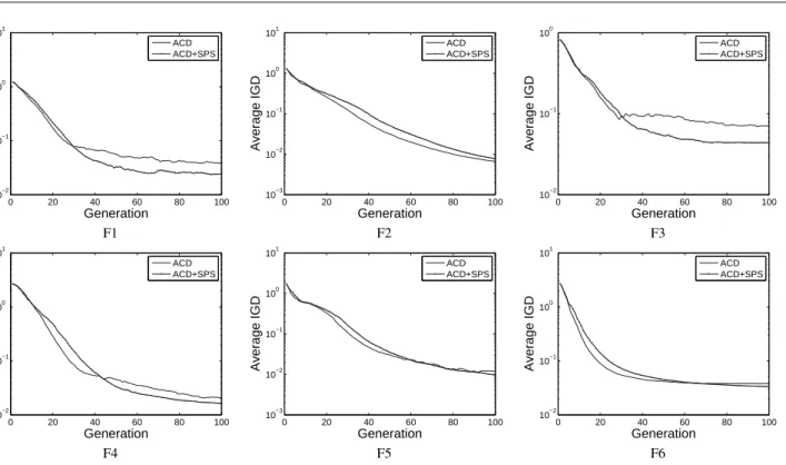
In order to have a better understanding of the impact of SPS, we graphically plot the average IGD metric obtained by ACD with and without SPS against the number of gen-erations on the six test problems in Fig. 9. Clearly, ACD without SPS generally has a faster convergence speed than that with SPS. The reason is that the use of SPS reduces the improvement region for each subproblem so that ACD+SPS needs some effort to find a new solution that is better, in

0 20 40 60 80 100 10−2 10−1 100 101 Generation Average IGD ACD ACD+SPS 0 20 40 60 80 100 10−3 10−2 10−1 100 101 Generation Average IGD ACD ACD+SPS 0 20 40 60 80 100 10−2 10−1 100 Generation Average IGD ACD ACD+SPS F1 F2 F3 0 20 40 60 80 100 10−2 10−1 100 101 Generation Average IGD ACD ACD+SPS 0 20 40 60 80 100 10−3 10−2 10−1 100 101 Generation Average IGD ACD ACD+SPS 0 20 40 60 80 100 10−2 10−1 100 101 Generation Average IGD ACD ACD+SPS F4 F5 F6

Fig. 9 Evolution curves of the average IGD metric for F1-F6.

terms of diversity and convergence, than the old solution of the considered subproblem and replace the old with the new one. Despite that, the use of SPS improves the IGD met-ric at the late stage for the problems except F2. This means that SPS enhances the diversity performance of MOEA/D-ACD, thereby providing improvement on the distribution of obtained POFs.

4.4.2 Integration into MOEA/D-STM

Another MOEA/D variant to be considered is a stable matching (STM) based MOEA, called MOEA/D-STM (Li et al., 2014c). MOEA/D-STM uses the STM model to coor-dinate the selection process in MOEA/D, where subproblem agents can express their preferences over the solution agents, and vice versa. As a consequence, suproblems’ preference encourages convergence whereas solutions’ preference pro-motes diversity. As our work focuses on the improvement of PBI, so PBI should be used in MOEA/D-STM for experi-mental analysis, and the penalty valueθis set to 5.0 (Zhang and Li, 2007). The other parameter settings remain the same as in Li et al. (2014c).

Table 5 reports the results of three performance mea-sures obtained by MOEA/D-STM and MOEA/D-STM with SPS, where for the notation convenience, “STM” and “STM+SPS” represent the former and the latter, respec-tively. It can be clearly observed that, the use of SPS sig-nificantly improves the performance of STM for all the con-sidered problems. On the other hand, it is worth noting that

Table 5 Best, mean and worst performance measure values obtained by STM and STM+SPS MS IGD HV Prob. STM STM+SPS ACD STM+SPS STM STM+SPS F1 0.5375 0.8960 0.1025 0.0188 1.3139 1.3351 0.5273 0.8676 0.1068 0.0221 1.3123 1.3346 0.5130 0.8186 0.1124 0.0338 1.3099 1.3326 F2 0.0000 1.0000 0.7838 0.0159 0.2400 0.5399 0.0000 1.0000 0.7838 0.0219 0.2400 0.5349 0.0000 1.0000 0.7838 0.0407 0.2400 0.5283 F3 0.4796 0.8822 0.1978 0.0211 1.3319 1.3560 0.3311 0.8770 0.4036 0.0252 1.2976 1.3547 0.3191 0.8407 0.4051 0.0331 1.2956 1.3526 F4 0.6579 0.9248 0.0805 0.0138 1.2538 1.2645 0.6066 0.8949 0.0846 0.0166 1.2525 1.2637 0.5998 0.8857 0.0861 0.0194 1.2519 1.2624 F5 0.8784 0.9817 0.0253 0.0114 0.7546 0.7618 0.8719 0.9478 0.0313 0.0154 0.7533 0.7598 0.8678 0.9370 0.0406 0.0206 0.7517 0.7578 F6 0.7373 1.0000 0.0389 0.0334 1.6693 1.6725 0.7094 1.0000 0.0421 0.0355 1.6664 1.6714 0.6847 0.9943 0.0444 0.0378 1.6625 1.6696

STM seems struggling to solve F2, and its MS metric value of zero indicates that STM produces as many duplicate so-lutions as the population size for F2. In contrast, when SPS is integrated into STM, F2 can be easily approximated, as indicated by the very small IGD values. This means a fixed penalty value for PBI in STM is not suitable for solving test problems.

The poor performance of STM without SPS on the tested problems may be explained by two possible reasons. One is

Table 6 Best, median and worst IGD values obtained by PBI+SPS with differentαvalues on F1 and F2

Prob. α= 1.0 α= 2.0 α= 3.0 α= 4.0 α= 5.0 α= 10.0 F1 0.1757 0.0791 0.0351 0.0181 0.0186 0.0193 0.1761 0.0825 0.0391 0.0213 0.0203 0.0219 0.1771 0.0877 0.0575 0.0288 0.0325 0.0287 F2 0.0047 0.0047 0.0047 0.0047 0.0048 0.0090 0.0048 0.0048 0.0048 0.0049 0.0052 0.0137 0.7835 0.7835 0.0071 0.0051 0.0067 0.0230

that, the test problems may be too complicated in terms of their POF shapes so that STM struggles to solve them. The other reason may be the inappropriate setting of the penalty value in PBI. As subproblems in MOEA/D are responsible for different landscapes of the objective space, they should be given different penalty values for different scenarios to balance convergence and diversity in PBI. Although STM promotes the balance between convergence and diversity, its convergence still depends on scalarizing functions. Thus, when PBI is chosen as the scalarizing function, the penalty value should be carefully specified.

4.5 Influence of Parameterαon SPS

In SPS, the magnitude of penalty for a subproblem consid-erably depends on its control parameterα. In this subsec-tion, we investigate the sensitivity of SPS to this parameter. MOEA/D with PBI+SPS is tested on F1 and F2 since these two problems have distinctly different POF shapes, i.e., F1 is extremely convex whereas F2 is extremely concave. The value ofαin SPS varies from 1.0 to 10.0, and other param-eters remain the same as in Section 4.1.

Table 6 presents the obtained IGD values of MOEA/D with PBI+SPS with differentαvalues on F1 and F2. It can be observed that, for F1,α = 4.0 in SPS provides better IGD values than the other settings. Settingαto a too small or too large value degrades the performance of PBI+SPS in terms of the IGD metric. For F2, however, all the settings ofαexceptα= 10.0can produce similar IGD results and there is no significant difference between these IGD values. This observation indirectly indicates that, concave problems are less likely to be affected by the penalty factorθin PBI, but this is not the case with convex problems.

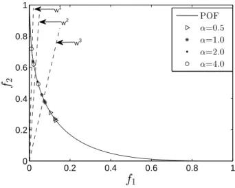
In SPS, the penalty value is controlled by two parame-ters, i.e.,αandβ. For a weight vectorwi_{,βi can be easily} calculated by Eq. (6). Thus,αis the only factor that can in-fluence the penalty value. However, for distinct weight vec-tors, the value ofαβmay be different. There are at least two scenarios, i.e.,αβ <1orαβ ≥1. Smallαβvalues under-emphasize population diversity whereas large ones favour diversity. To investigate these situations, we use F1 as the test problem. As F1 has an extremely convex POF shape, the boundary regions are hard to be located. Therefore, we

0 0.2 0.4 0.6 0.8 1 0 0.2 0.4 0.6 0.8 1

f

f

Fig. 10 Influence ofαon population distribution for F1.

select three boundary weight vectorsw1

= (0.02,0.98)T_, w2

= (0.05,0.95)T _andw3

= (0.15,0.85)T _to approxi-mate three boundary points. Correspondingly, theirβvalues areβ1= 0.96,β2= 0.9, andβ3= 0.7, respectively.αis set

asα=0.5, 1, 2, and 4, meaning thatαβ <1ifα=0.5 and 1; otherwise,αβ >1. Since only three population individuals (which is determined by the number of weight vectors) are used, we increase the maximum number of generations to 1000 in order to guarantee convergence.

Figure 10 shows the influence ofαon population dis-tribution. Clearly, the largerαis, the more spread the ob-tained points will be. Thus,α= 4yields better spread than the other settings, although one of the solutions is a little bit far away fromw3

. We guess thatα = 4might be too large for the subproblem associated with w3

, which may discard solutions that have good convergence but poor diver-sity. On the other hand, smallαvalues favour intermediate points as these points are much closer than boundary points to the ideal point, indicating that the resulting penalty is not enough to maintain diversity.

It is worth noting thatα= 4.0might not be the best pa-rameter setting for all kinds of problems, although it clearly provides a significant improvement for PBI. Asαcontrols the balance between the population diversity and conver-gence for each decomposed subproblem, it should be care-fully selected in order to maximize the algorithm’s perfor-mance. Also, it is desirable to design an adaptive strategy for the setting ofα, which is left for our future work.

5 Conclusions and Future Work

In this paper we have investigated the influence of the penalty factor on the performance of PBI within MOEA/D. The investigation shows that, a small penalty value is

bene-ficial for convergence but may make PBI unable to preserve boundary solutions if boundary solutions are much further away from the obtained ideal point than intermediate solu-tions, while a large one is advantageous to diversity but can slow down the convergence course. On the basis of this in-vestigation, two new penalty schemes, i.e., APS and SPS, are introduced to strike a balance between convergence and diversity. Similar to the original PBI, APS assigns identical penalty values for all subproblems, but the penalty values are generationally increasing during the course of search, with a small value at the early stage in favour of fast conver-gence and a large one at the late stage emphasizing diversity and spread of solutions. In contrast, SPS turns to specify distinct penalty values for different subproblems according to the location of their associated weight vectors. Boundary subproblems are given a strict penalty and intermediate ones are given a loose penalty. This way, preservation of bound-ary solutions are enhanced so as to provide a wide spread of Pareto font.

These two new penalty schemes have been tested on several complex problems, including bi-objective and three-objective problems. Experimental studies have shown that both schemes help ease the loss of boundary solutions and outspread the Pareto font, and PBI with SPS performs sig-nificantly better than that with APS. This means SPS is an effective way to improve the performance of PBI. Be-sides, SPS has been integrated into two recently proposed variants of MOEA/D, i.e., ACD and MOEA/D-STM, and experimental results have clearly demonstrated the efficiency of SPS in promoting the performance of decomposition-based MOEAs with PBI.

Although the proposed penalty schemes have offered en-couraging results on the test problems considered in this pa-per, they should be examined on a wider range of different kinds of problems. As there has recently been an increas-ing number of studies in extendincreas-ing PBI-based MOEAs to many-objective optimization, it should be very interesting to further examine the effect of PBI on different types of many-objective problems. Besides, designing a parameter-free or adaptive PBI method for MOEA/D is very desirable. In our future work, MOEA/D with PBI variants will be compared with other state-of-the-art algorithms.

Acknowledgement

This work was supported by the Engineering and Physical Sciences Research Council (EPSRC) of U.K. under Grant EP/K001310/1 and the National Natural Science Foundation of China under Grant 61273031.

References

Al Moubayed N, Petrovski A, McCall J (2013) D2

M OP SO: MOPSO based on decomposition and dominance with archiving using crowding distance in objective and solution spaces. Evol Comput 22(1):47–77 Asafuddoula M, Ray T, Sarker R (2015) A decomposition

based evolutionary algorithm for many objective opti-mization. IEEE Trans Evol Comput 19(3):445–460 Beume N, Naujoks N, Emmerich M (2007) SMS-EMOA:

Multiobjective selection based on dominated hypervol-ume. Eur J Oper Res 181(3):1653–1669

Bader J, Zitzler E (2011) HypE: An algorithm for fast hypervolume-based many-objective optimization. Evol Comput 19(1):45–76

Cheng R, Jin Y, Narukawa K (2015) Adaptive reference vec-tor generation for inverse model based evolutionary multi-objective optimization with degenerate and disconnected Pareto fronts. In: Evolutionary Multi-Criterion Optimiza-tion (EMO 2015), Part I, LNCS 9018, pp 127–140 Cheng R, Jin Y, Olhofer M, Sendhoff B (2016). A reference

vector guided evolutionary algorithm for many-objective optimization. IEEE Trans Evol Comput (in press), doi: 10.1109/TEVC.2016.2519378

Chikumbo O, Goodman ED, Deb K (2012) Approximating a multi-dimensional pareto front for a land use management problem: A modified moea with an epigenetic silencing metaphor. In: Proceedings of 2012 IEEE Congress on Evolutionary Computation (CEC 2012), pp 1–9

Deb K, Agrawwal S, Pratap A, Meyarivan T (2002) A fast and elitist multiobjective genetic algorithm: NSGA-II. IEEE Trans Evol Comput 6(2):182–197

Deb K, Jain H (2014) An evolutionary many-Objective op-timization algorithm using reference-point based non-dominated sorting approach, Part I: Solving prob-lems with box constraints. IEEE Trans Evol Comput 18(4):577–601

Deb K, Pratap A, Moitra S (2000) Mechanical component design for multiple objectives using elitist non-dominated sorting GA. In: Proceedings of the 6th International Con-ference on Parallel Problem Solving from Nature (PPSN VI), pp 859–868

Deb K, Thiele L, Laumanns M, Zitzler E (2005) Scable test problems for evolutionary multi-objective optimization. In: Abraham A, Jain L, Goldberg R (Eds.) Evolutionary Multiobjective Optimization: Theoretical Advances and Applications, Springer, London, pp 105–145

Giagkiozis I, Purshouse RC, Fleming PJ (2014) General-ized decomposition and cross entropy methods for many-objective optimization. Inform Sci 282:363–387

Goh C, Tan KC (2007) An investigation on noisy environ-ments in evolutionary multiobjective optimization. IEEE Trans Evol Comput 11(3):354–381

Gomez RH, Coello Coello CA (2015) Improved metaheuris-tic based on the r2 indicator for many-objective optimiza-tion. In: Proceedings of the 2015 Genetic and Evolution-ary Computation Conference (GECCO 15), pp 679–686 Huband S, Hingston P, Barone L, While L (2006) A review

of multiobjective test problems and a scalable test prob-lem toolkit. IEEE Trans Evol Comput 10(2):477–506 Ishibuchi H, Akedo N, Nojima Y (2015) Behavior of

multi-objective evolutionary algorithms on many-multi-objective knapsack problems. IEEE Trans Evol Comput 19(2):264– 283

Ishibuchi H, Akedo N, Nojima Y (2013) A study on the specification of a scalarizing function in MOEA/D for many-objective knapsack problems. In: Proceedings of the 7th International Conference on Learning and Intelli-gent Optimization 7 (LION 7), LNCS 7997, pp 231–246 Ishibuchi H, Tsukamoto N, Hitotsuyanagi Y, Nojima Y

(2010) Indicator-based evolutionary algorithm with hy-pervolume approximation by achievement scalarizing function. In: Proceedings of 12th Annual Conference on Genetic Evolutionary Computation (GECCO 2010), pp 527–534

Jain H, Deb K (2014) An improved adaptive approach for elitist nondominated sorting genetic algorithm for many-objective optimization. In: Evolutionary Multi-Criterion Optimization (EMO 2013), LNCS 7811, pp 307–321 Jia S, Zhu J, Du B, Yue H (2011) Indicator-based particle

swarm optimization with local search. In: Proceedings of the 7th International Conference on Natural Computation, pp 1180–1184

Jiang S, Yang S (2016) An improved multi-objective op-timization evolutionary algorithm based on decompo-sition for complex Pareto fronts. IEEE Trans Cybern. 46(2):421-437

Knowles JD, Corne DW (1999) The pareto archived evolu-tion strategy: A new baseline algorithm for multiobjective optimisation. In: Proceedings of the 1999 IEEE Congress on Evolutionary Computation (CEC 1999), pp 98–105 Li B, Li J, Tang K, Yao X (2014a) An improved two archive

algorithm for many-objective optimization. In: Proceed-ings of the 2014 IEEE Congress on Evolutionary Compu-tation (CEC 2014), pp 2869–2876

Li K, Deb K, Zhang Q, Kwong S (2015a) An evolutionary many-Objective optimization algorithm based on dom-inance and decomposition. IEEE Trans Evol Comput 19(5):694–716

Li K, Fialho A, Kwong S, Zhang Q (2014b) Adaptive op-erator selection with bandits for multiobjective evolution-ary algorithm based on decomposition. IEEE Trans Evol Comput 18(1):114–130

Li K, Kwong S, Zhang Q, Deb K (2015b) Interrelationship-based selection for decomposition multiobjective opti-mization. IEEE Trans Cybern 45(10):2076–2088

Li K, Zhang Q, Kwong S, Li M, Wang R (2014c) Stable matching based selection in evolutionary multiobjective optimization. IEEE Trans Evol Comput 18(6):909–923 Li H, Zhang Q (2009) Multiobjective optimization problems

with complicated pareto sets, MOEA/D and NSGA-II. IEEE Trans Evol Comput 13(2):284–302

Liu H, Gu F, Zhang Q (2014) Decomposition of a mul-tiobjective optimization problem into a number of sim-ple multiobjective subproblems. IEEE Trans Evol Com-put 18(3):450–455

Masoomi Z, Mesgari MS, Hamrah M (2013) Allocation of urban land uses by multi-objective particle swarm opti-mization algorithm. Int J Geogr Inf Sci 27(3):542–565 Mendez AM, Coello Coello CA (2015) GD-MOEA: A new

multi-objective evolutionary algorithm on the generation distance indicator, In: Evolutionary Multi-Criterion Opti-mization, LNCS 9018, pp 156–170

Mohammadi A, Omidvar MN, Li X, Deb K (2014) In-tegrating user preferences and decomposition methods for many-objective optimization. In: Proceedings of the 2014 IEEE Congress on Evolutionary Computation (CEC 2014), pp 421–428

Osycza A, Kundu S (1995) A new method to solve general-ized multicriteria optimization problems using the simple genetic algorithm. Struct Optimization 10(2):94–99 Pavelski LM, Delgado MR, de Almeida CP, Goncalves RA,

Venske SM (2014) ELMOEA/D-DE: Extreme learning surrogate models in multi-objective optimization based on decomposition and differential evolution. In: Proceed-ings of the 2014 Brazilian Conference on Intelligent Sys-tems (BRACIS), pp 318–323

Qi T, Ma X, Liu F, Jiao L, Sun J, Wu J (2014) MOEA/D with adaptive weight adjustment. Evol Comput 22(2):231–264 Reed PM, Hadka D, Herman JD, Kasprzyk JR, Kollat JB (2013) Evolutionary multiobjective in water resources: The past, present, and future. Adv Water Resour 51:438– 456

Sato H (2014) Inverted PBI in MOEA/D and its impact on the search performance on multi and many-objective opti-mization. In: Proceedings of the 2014 Annual Conference on Genetic and Evolutionary Computation (GECCO 14), pp 645–652

Wang G, Chen J, Cai T, Xin B (2013) Decomposition-based multi-objective differential evolution particle swarm opti-mization for the design of tubular permanent magnet lin-ear synchronous motor. Eng Optimiz 45(9):1107–1127 Wang L, Zhang Q, Zhou A, Gong M, Jiao L (2015)

Con-strained subproblems in decomposition based multiobjec-tive evolutionary algorithm. IEEE Trans Evol Comput (in press), doi:10.1109/TEVC.2015.2457616

Yang XS, Deb S (2013) Multiobjective cuckoo search for design optimization. Comput Oper Res 40(6):1616–1624

Yuan Y, Xu H, Wang B (2014) Evolutionary many-objective optimization using ensemble fitness ranking. In: Proceed-ings of the 2014 Annual Conference on Genetic and Evo-lutionary Computation (GECCO 2014), pp 669–676 Yuan Y, Xu H, Wang B, Yao X (2015) A new dominance

relation based evolutionary algorithm for many-objective optimization. IEEE Trans Evol Comput. 20(1):16–37 Zhang Q and Li H (2007) MOEA/D: A multiobjective

evo-lutionary algorithm based on decomposition. IEEE Trans Evol Comput 11(6):712–731

Zitzler E, Deb K, Thiele L (2000) Comparison of multiob-jective evolutionary algorithms: Empirical results. Evol Comput 8(2):173–195

Zitzler E, Kunzli S (2004) Indicator-based selection in mul-tiobjective search. In: Proceedings of the 8th Interna-tional Conference on Parallel Problem Solving from Na-ture (PPSN VIII), vol 3242, pp 832–842

Zitzler E, Laumanns M, Thiele L (2002) SPEA2: Improv-ing the strength Pareto evolutionary algorithm for mul-tiobjective optimization. In: Proceedings of Evolutionary Methods for Design, Optimisation and Control with Ap-plication to Industrial Problems (EUROGEN 2001), vol 3242, no 103, pp 95–100

Zitzler E, Thiele L (1999) Multiobjective evolutionary algo-rithms: A comparative case study and the strength pareto approach. IEEE Trans Evol Comput 3(4):257–271 Zitzler E, Thiele L, Laumanns M, Fonseca CM, da Fonseca

VG (2003) Performance assessment of multiobjective op-timizers: An analysis and review. IEEE Trans Evol Com-put 7(2):117–132