Synchronised Demand-Capacity Balancing in
Collaborative Air Traffic Flow Management
Yan Xua,b, Xavier Pratsb, Daniel Delahayec
aCentre for Aeronautics, School of Aerospace, Transport and Manufacturing, Cranfield
University, Cranfield MK43 0AL, Bedford (UK)
bDepartment of Physics - Aeronautics Division, Technical University of Catalonia,
Castelldefels 08860, Barcelona (Spain)
cOPTIM Group, ENAC Laboratory, Ecole Nationale de l’Aviation Civile, 7 Avenue
Edouard Belin, 31400 Toulouse (France)
Abstract
This paper introduces a novel approach for synchronised demand-capacity balancing within a proposed Collaborative Air Traffic Flow Management framework. The approach is aimed to realise optimising traffic flow and scheduling airspace configuration in a more harmonised manner. Options such as delay assignment and alternative trajectories (generated and submit-ted by Airspace Users) are intended for regulating the traffic flow. Airspace reconfiguration involves, on the other side, adjusting the opening schemes of predefined configurations, or creating new ones (if needed) through dy-namic sectorisation. Results suggest that, using the proposed approach, the required system delay can be reduced remarkably, whereas the number of opened sectors (and thus operating cost) and the total capacity provision (supplied by the Air Navigation Service Providers) decrease at the same time, due to the increased capacity utilisation per operating sector.
Keywords: air traffic flow management, collaborative demand and capacity balancing, trajectory options, airspace configuration, sectorisation
Nomenclature
f ∈ F set of flights
j ∈ J set of elementary sectors
k∈ K set of trajectory options
t∈ T set of time moments
τ ∈T set of time periods l∈ L set of operating sectors
a∈ A set of area control centers
s∈ S set of airspace configurations
Kf subset of trajectory options submitted by flightf
Jk
f subset of elementary sectors flightf (or trajectory k) traverses
Tfk,j subset of time feasible for flightf (or trajectory k) entering elementary sectorj
T(τ) subset of time moments subject to time periodτ
Lτ subset of operating sectors opened in time periodτ
Lj subset of operating sectors constructed by elementary sectorj
Jl subset of elementary sectors in operating sectorl
Sl subset of airspace configurations constructed by operating sector l
Sa subset of airspace configurations belonged to area control centera
Jf,lk,τ 1st elementary sector for flightf (or trajectory k) that functions in operating sectorl in time periodτ
Jk
f(i) ith elementary sector for flight f (or trajectory k)
Tk,jf upper bound of feasible time windowTfk,j Tk,jf lower bound of feasible time windowTfk,j
rk,jf estimated arrival time of flightf (or trajectory k) entering elementary sectorj
nkf total no. of elementary sectors flightf (or trajectory k) traverses ˆ
tk,jjf 0 scheduled flight time of segmentjj0 for flight f (orkth trajectory)
cτl capacity of operating sectorl during time periodτ dkf extra fuel consumption forkth trajectory of flightf ek
f extra route charges forkth trajectory of flightf α unit cost of performing ground delay
γ unit cost of fuel consumption
δ unit cost of opening an operating sector
1. Introduction
Year 2016 saw an average departure delay per flight of 11.3 minutes in Europe, an increase of 9% in comparison to 2015. It was recorded with an average of 1.9% for operational cancellation monthly, and the percentage of flights delayed more than 30 minutes from all-causes increased to 9.8% ( Eu-rocontrol, 2017). In the U.S., 17% of the flights were delayed by more than 15 minutes in 2016, with another 1.2% cancelled (US Department of Trans-portation,2016). China suffers severe flight delays too, reporting an average of 16 minutes and 21 minutes in 2016 and in 2015 respectively (CAAC,2016). Indeed, such problems have been observed not only in these regions, but also in various places across the world.
One of the primary causes for these delays is that the number of flights (demand) often exceeds the supply of the airspace/airport accommodation (capacity). The effort thereby to achieve demand-capacity balancing (DCB) is typically known as air traffic flow management (ATFM) (Bertsimas and Patterson, 1998). Following the pioneering work done by Odoni (1987), a number of researchers have focused their activity on the development of ground delay assignment as a short-term measure in response to capacity reduction at the arrival airport (Terrab and Paulose, 1992). Taking into ac-count the capacity constraints from airspace sectors, the problem of control-ling release times and speed adjustments of aircraft for a network of airports and sectors has been discussed in (Lulli and Odoni,2007). Thereafter, Bert-simas et al. (2011) further introduced new constraints to the well-studied ATFM model in (Bertsimas and Patterson, 1998) that forced local routing conditions sufficient to perform the rerouting function efficiently.
In the U.S., ATFM programs include Ground Delay Programs (GDPs) and Airspace Flow Programs (AFPs), led by the Federal Aviation Admin-istration (FAA, 2009). GDPs control the arrival rate at an affected (desti-nation) airport by assigning departure delays to flights (FAA, 2009). Like-wise, an AFP identifies constraints in the en-route system, regulating flights crossing a given Flow Constrained Area (FCA) (Libby et al., 2005). Sim-ilar initiatives exist in Europe, implemented by the Eurocontrol’s Network Manager (NM) Operations Centre (previously known as the central flow man-agement unit). Eurocontrol has been advancing these initiatives through the development of User Driven Prioritisation Process (UDPP) to enable addi-tional flexibility for airspace users (AUs) to adapt their operations in a more cost-efficient manner (SESAR, 2015). On the basis of GDP/AFP, a newly
introduced Collaborative Trajectory Options Program (CTOP) has been re-cently deployed in the U.S., which could handle multiple FCAs in a single program (FAA, 2014). Increased collaborative decision-making (CDM), as its benefits detailed in (Ball et al., 2000), can be found in CTOP, wherein it allows AUs to submit a set of preferred trajectories, i.e. trajectory options set (TOS), prior to the issuance of the program (Miller and Hall,2015).
The airspace system nowadays is usually partitioned into sectors, each of which is handled by a group of air traffic controllers (ATCO) and is bonded with a limited capacity. In the past, such airspace sectorisation was con-ducted in an empirical way in which airspace experts apply rules they have learned from experience. However, as mentioned in (Kopardekar et al.,2007), some of these capacity resources might be under-utilised and lack of flexibil-ity, thus requiring a better reorganisation. For the last decades, researchers have proposed automatic sector definition methods by using evolutionary al-gorithms to address the classical graph partitioning problem (see (Delahaye et al., 1994, 1998) for instance). Due to practical issues (e.g., ATCO train-ing), current sectorisation is mostly realised by choosing the best opening scheme for a predefined set of configurations, namely redefining the existing sectors to better account for the traffic flow (FAA,2002). More ambitious al-ternatives encompass the concept of dynamic airspace configuration (DAC), in which airspace (capacity) is adjusted in real time to accommodate the demand that may evolve throughout a given day (Sherali and Hill, 2013).
Typically, the above-mentioned initiatives for flow management and for airspace sectorisation are done independently, by respectively the ATFM unit (such as the NM in Europe) and the local Air Navigation Service Provider (ANSP), which might be not well coordinated or synchronised. One implicit problem is that the given airspace sectorisation is often designed to best ac-commodate the traffic flow patterns formed by the planned (or historical) demand. Once these flight trajectories have been changed, due to DCB (ei-ther by imposing delays or reroutings), the temporal-spatial flow patterns will then change, and consequently the initial sectorisation may be not optimal.
In this paper, we explore the potential of synchronising the traffic flow optimisation and the airspace configuration scheduling. Four model variants are presented and compared, showing the effects of such harmonisation for achieving better DCB performance. The first model is focused on regulating traffic flow by means of assigning delays. Alternative trajectory options, similar to the concept of TOS in CTOP, are then included to the second model, in such a way that demand can be managed in both time and space
margins. Next, the third model releases the constraint of maintaining the initial sectorisation, allowing flexible sector opening to some extent. Finally, instead of using the existing airspace configurations, the last model optimises the collapsing architecture of the elementary sectors, therefore creating new configurations if needed.
2. Motivation
In previous work (Xu and Prats,2017), we investigated an approach com-bining different delay management initiatives, including ground holding, air-borne holding, linear holding and delay recovery (see Fig. 1a) into an in-tegrated DCB model, such that the cost efficiency of delay assignment can be improved. Then, based on this model, a follow-up work (Xu et al., 2018) demonstrated a remarkable delay reduction when further incorporating al-ternative trajectory options, which were intended to bypass the identified hotspot areas (i.e. airspace sectors with demand exceeding the capacity) as shown in Fig. 1b. All these initiatives, however, are focused on the demand side, through regulating the traffic flow, i.e., assigning delays (in different forms) and using alternative trajectories. The airspace sectorisation, mean-while, remained unchanged than initially planned.
Let us take a look at a simple example in Fig. 1c and Fig. 1dwhere the airspace sectorisation is fixed and the other is subject to flexible adjustment. For the original flight plans, more operators prefer to schedule a flight route, as coloured in red, to fly from Rome (LIRF) to Amsterdam (EHAM). Ac-cordingly, for the two areas labelled out in the map, as shown in Fig. 1c, the one crossed by the congested route is divided to four sectors (for instance) operating at the same time to provide more capacities, whereas the other area is operated by only one sector as a whole.
However, having been through some DCB initiatives, certain amount of flights could be diverted to the route coloured in green (see Fig. 1d), and some flights could be assigned with certain delays such that their Controlled Times of Arrival (CTAs) at that area might be changed (and sequenced) as well. That is to say, the previous congested area becomes less demanded for capacity. It is beneficial to merge the former four sectors to one entire sector so as to reduce the extra operating costs, and meanwhile, to diverge the previously less-congested area from one sector to two smaller sectors to better handle the additional traffic demand. Up to the best of our knowledge,
no previous work has explicitly addressed this issue, namely the optimisation of both delays/trajectories and sectorisation in a single framework.
(a) Assigning delays
EHAM
LIRF
Alternative
Original
(b) Allowing alternative trajectories
EHAM
LIRF
4 sectors
1 sector
(c) Fixed airspace sectorisation
EHAM
LIRF
1 sector
2 sectors
(d) Adjusting airspace sectorisation Figure 1: Illustration of initiatives taken for balancing demand and capacity.
3. Model components
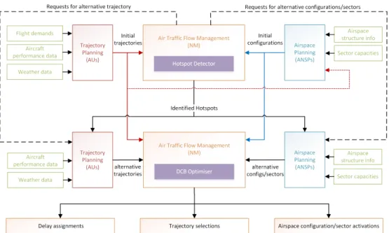
Following the above thought, this section introduces a synchronised col-laborative DCB (SC-DCB) model. The overall architecture is composed of a set of functional components, and the corresponding work flow is as pre-sented in Fig. 2. For convenience, the main stakeholders involved are limited to the scope of AUs, ANSPs and the NM, although in real operations more comprehensive collaborations with other stakeholders may be required.
Figure 2: An overview of the architecture and work flow for the proposed model framework.
3.1. Overall framework
The main functions of each model component are described below. It should be noted that the first two specific components (i.e., initial schedul-ing of user-preferred trajectory and airspace configuration) are aimed at the model initialisation process. As the main objective of this paper is to demon-strate the inefficiencies of current operations and to propose a possible way to better understand and to address such inefficiencies, these initialisations will follow current operations and are out of the discussion of this paper. Mean-while, the modular design of the proposed framework allows other method-ologies to apply in these components, and the reader may direct to the men-tioned work (and the references therein) for more details.
• Initial scheduling of user-preferred trajectory: It enables the scheduling of the initial 4D trajectories to well reflect AUs’ preferences (e.g., minimising the direct operating cost including fuel consumption, time related costs, route charges etc.). The trajectory optimisation and planning methodology used in this component has been previously reported in (Dalmau et al., 2018).
traf-fic sample and airspace sectorisation with operational limitations, it generates an optimal sector opening scheme mimicking what the Air Navigation Service Providers (ANSPs) would do, i.e., an optimal list of airspace configurations or optimal grouping of sectors for each period of time (see (Gianazza,2007) for instance).
• Detection of time-varying hotspot airspaces: According to the initial trajectories and the initial airspace configurations (and nominal capacity allocations) derived from the previous two components re-spectively, the time-varying hotspot volumes will be identified, by the NM in this model component, capturing the airspaces where demand exceeds capacity (see Sec. 3.2).
• Submission of alternative trajectory options: In this part, the AUs are allowed to submit (if desired) some alternative trajectories, based on the detected hotspots and/or the latest aeronautical infor-mation, for their flights that are scheduled to traverse the identified hotspots and/or are affected by the updated situations (see Sec. 3.3).
• Provision of available airspace adjustments: For those identified hotspots, the available adjustments (in terms of the airspace sectorisa-tion) will be provided through the concerned ANSPs in charge of the areas in line with their cost breakdown policies (see Sec. 3.4).
• Integrated optimisation model for synchronised DCB:With the above possible options collected, the last model component is to com-pute, as done by the NM, the best trajectory selection and distribution of delay for all the flights, as well as the optimal airspace configuration across the whole area during each period of time (see Sec. 4).
Wrapping up, the general work flow starts from AUs and ANSPs schedul-ing the initial set of flight trajectories (demand) and airspace configurations (capacity). Then, the NM identifies the hotspots based on the initial de-mand and capacity, and thus requests possible alternative options, whilst distributing some latest information which assists in better decision making from AUs and ANSPs who could both share their alternative intentions. Fi-nally, a centralised solution will be provided by the NM based on knowing the whole picture of all available options, producing the optimal trajectory selec-tions and airspace configuraselec-tions/sector activaselec-tions, as well as the required delay assignments, with the objective of minimising the total operating cost.
3.2. Detection of time-varying hotspot airspaces
Given the initially planned flight trajectories and airspace opening schemes (and the corresponding capacity provisions), the primary demand and capac-ity situations can be assessed. The entry rate (into an airspace sector) is used as the way of counting traffic demand in this paper, whilst the sectors’ thresh-old values are retrieved as the operating capacities. The airspace sector is typically defined as a 3D volume (geographical boundaries with lower and upper altitudes), and the hotspot airspace (sector) is further identified within a certain period of activation time, thus turning to be a 4D volume, in which the traffic demand is higher than the capacity. As both demand and capacity are dependent on time, namely in form of the 4D trajectories and the open-ing schemes of configurations respectively, the identified hotspots are hence time-varying as well. An intuitive example is shown in Fig. 3, where, for convenience, only the projected horizontal 2D hotspots are presented, and we can see that the hotspots’ locations could vary notably in 20 minutes (based on the counted aircraft entry rate and sector operating capacity that is typically given in every 20/60 minutes). Note that, in the defined airspace network, the sector entrance represents the node whilst the structured air routes are the edges connecting each node across the network.
(a) 10:00 AM - 10:20 AM (b) 10:20 AM - 10:40 AM
Figure 3: Time-varying projected hotspot volumes identified across the airspace network.
Subsequently, the flights scheduled to traverse those hotspot volumes can be captured. To avoid entering into a hotspot, it is possible to simply impose delays to a flight (which is commonly-seen nowadays), or to reroute it out of the concerned area. In this paper, both lateral- and vertical-avoidance
strategies to bypass an airspace volume are proposed. Although several vol-umes might be detected across the network for the same period of time (see Fig. 3), the captured flights only need to bypass the 4D volumes that they are scheduled to traverse, without taking into account all the hotspots (as they are time-varying).
The rerouting strategy (either in lateral or vertical domains) sometimes could be inefficient (e.g., too high operating costs) for AUs, such that the incentives of participating in the collaborative decision-making process may be declined. For the purpose of incurring as few extra costs as possible (in comparison with the initial trajectory), this model component consists of sharing some additional hotspot-avoidance information to the AUs for each captured flight, as explained below.
In terms of the lateral avoidance, the boundary coordinates of each air-block are given in such a way that a specific polygon graph can be formed on the horizontal plane representing each hotspot’s lateral area. The alternative trajectory must avoid to intersect with any of the connecting frontiers (linked through the boundaries). For the vertical-avoidance, the flight is informed at which distance it should start to change the initial altitude and at which dis-tance to recover that altitude (if desired), as well as the non-selectable flight levels between the two distances. Such guidance is given for each sector that the initial trajectory needs to bypass. This set of avoidance information will be then utilised in the next model component.
3.3. Submission of alternative trajectory options
In Sec. 3.2, we have introduced a way to share the hotspot-avoidance information, aiming to assist AUs to better schedule their alternative tra-jectories with as few extra costs as possible. Once receiving this avoidance information, AUs could produce the alternative trajectories for their affected flights, using exactly the same method when planning the initial trajectories but with additional constraints (as specified in the avoidance information) incorporated in the trajectory optimisation model. For more details about the method, the reader may direct to (Xu et al., 2018). Figs. 4a and 4b
represent that the AUs can take advantage of such shared avoidance infor-mation (see the red hotspot areas shown in the figures) provided by the NM, and then generate the optimal alternative trajectory bypassing the identified hotspots in lateral and vertical direction respectively.
In addition to the above hotspot-avoidance trajectories, alternatives for any other specific purposes are also applicable. For instance, the
meteoro-Initial trajectory Lateral alternative Hotspots
(a) Lateral hotspot avoidance (b) Vertical hotspot avoidance
Initial trajectory GCD
(c) Wind field prediction (d) Experienced ATC restriction
Figure 4: Different types of alternative trajectory options with different purposes.
logical conditions and forecasts usually become more accurate as the take-off time approaches, and thus it could be more efficient to fly a new trajectory taking advantage of the updated predictions such as the wind fields (see Fig. 4c and compare the great circle distance between two airports with the wind-optimal trajectory for a given day). Besides, tactical ATCO’s in-structions (resulted from flexible airspace usage for instance) might affect the climb/descent phases or specify short-cut routes to smooth the traffic flow in the terminal airspace. The executed trajectory may partly differ than the initial trajectory, as sometimes AUs will not be given with this information when planning their flights. It would be helpful to consider these actions based on the latest predictions, in such a way that an updated trajectory can be planned prior to real execution. As an example, Fig. 4dillustrates a
suboptimal (compared to the initial) trajectory taking account a step descent procedure (which could be also modelled in the methodology).
To sum up, in the proposed model, AUs are invited to freely submit a set of preferred trajectories (see Table1), along with the corresponding extra costs with respect to their initial trajectories. However, the method of how to outline a workable collaborative mechanism (such as data sharing and incentive design) in realities still needs more discussion, and we assume in this paper that AUs can (and are willing) to correctly share this (proprietary) cost information. Despite of this, it should be noted that the submission of alternatives shall not be mandatory for the AUs, who could keep solely the initial, which will be likely subject to possible (significant) delays.
Table 1: Possible trajectory options submitted for one flight.
Options Extra costs Comments
Trajectory 0 0 Initial trajectory
Trajectory 1 Cost 1 Lateral hotspot avoidance
Trajectory 2 Cost 2 Vertical hotspot avoidance
Trajectory 3 Cost 3 Updated wind field prediction
Trajectory 4 Cost 4 Potential ATC action areas
..
. ... ...
Trajectory n Cost n Any specific preference
3.4. Provision of available airspace adjustments
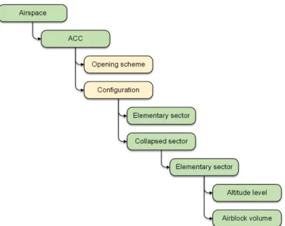
In line with the European airspace structure, as shown in Fig. 5, typically a large piece of airspace consists of several Area Control Centers (ACCs). Under current operations, each ACC normally operates independently, and has a certain amount of predefined configurations and corresponding opening schemes. Next, each specified configuration is composed of several elementary sectors and/or collapsed sectors, and each collapsed sector is in turn merged by several smaller elementary sectors. The small elementary sector is defined (in a long-term time scale) by a certain number of basic airblock volumes.
Consider a 3D block of airspace filled by non-overlapping elementary sec-tors. With the timeline added to the 4D scenario, sometimes a small elemen-tary sector itself functions as an operating sector, and at another time it is merged into a larger collapsed sector that acts as another operating sector. Moreover, each operating sector is bonded with certain operating capacity,
Figure 5: Schematic of airspace structure implemented in the Eurocontrol area.
which could be also associated with the Traffic Volumes where regulations can be applied (see more details in (Melgosa et al., 2019)).
Then, recall the airspace structure shown in Fig. 5. There could be at least the following levels to realise flexible airspace sectorisation:
• Level-i: Schedule airspace configurations’ opening schemes;
• Level-ii: Schedule operating sectors’ opening schemes, creating new airspace configuration when necessary;
• Level-iii: Schedule elementary sectors’ opening schemes, creating new operating sectors when necessary; and
• Level-iv: Design elementary sectors, creating new elementary sectors when necessary.
Specifically, the above methods could provide increasingly precise insights into the sectorisation problem, and thus result in more efficient airspace set-tings. However, incorporating these approaches, e.g., designing new elemen-tary sector (or even the airblocks) as done in (Delahaye et al., 1998), into the model may largely increase the computational burden, while several chal-lenges for the relevant DAC problem have been also marked in (Klein et al.,
2008). Note that this model is aimed to optimise not only sectorisation but also traffic flow. Hence, in this paper we only discuss the methods with less complexity, i.e., Level-i and Level-ii, scheduling the opening schemes for the already existing configurations or the existing operating sectors, without changing the geographical shape of any collapsed or elementary sector.
LFFFTM
(a) LFFFCTAE: Conf. 10B
LFFFTML
(b) LFFFCTAE: Conf. 10F
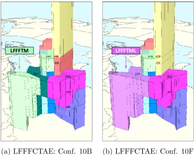
Figure 6: Operating sectors consisted in configurations 10B and 10F for ACC LFFFCTAE.
We can see an example in Fig. 6, where the elementary sector LFFFTM has been captured as a hotspot (within a certain period of time), and it acts as an independent operating sector (light green block in Fig. 6a) in configuration “10B” of the ACC LFFFCTAE. An available adjustment is that this elementary sector could be merged into the collapsed sector LFFFTML (purple block in Fig. 6b) when this ACC’s configuration “10F” is activated. As mentioned in Sec. 3.2, the time-varying hotspots are identified, so that the concerned ANSPs will be advised to share the available adjustments for their responsible sectors (based on the hotspots). The main effects of such dynamic sectorisation method are two folds:
• It enables flexible capacity provision, meaning that capacities can be re-allocated from free areas to some newly congested areas that may have been caused by traffic flow regulations; and
• It allows changes made on the collapsing architecture of elementary sectors, which will affect the way traffic demand is counted (i.e., entry rate) for the operating sectors.
Wrapping up, all the above derived “alternative trajectory options” in Sec. 3.3 and “available airspace adjustments” in Sec. 3.4 will be taken into account for an integrated optimisation model as presented in the next section.
4. Integrated optimisation models
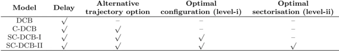
In line with the previous discussion, we present four variants of the pro-posed model to demonstrate the effects of this trajectory-airspace synchro-nisation in DCB: a Baseline Model DCB, a Benchmark Model C-DCB and two Full-functional models SC-DCB-I and SC-DCB-II. Next sections detail these models, shown as well in Table 2, which summarises the main feature (or initiative) activated in each model.
Table 2: Initiatives of the four model variants considered in this study.
Model Delay Alternative
trajectory option Optimal configuration (level-i) Optimal sectorisation (level-ii) DCB √ – – – C-DCB √ √ – – SC-DCB-I √ √ √ – SC-DCB-II √ √ √ √ 4.1. Baseline Model DCB
Model DCB aims at balancing demand under capacity through assign-ing ground delay to flights. A set of fixed airspace openassign-ing schemes (with changeable configurations throughout periods of time) are considered, which are planned in early stage based on the historical traffic flow. Aiming at future trajectory based operations, controlled times of arrival (CTAs) are imposed at each control point along the trajectory, which, in turn, is de-fined at the entrance position of each elementary sector that the trajectory is scheduled to traverse. Subsequently, to assign the CTAs, we consider a set of decision variables as follows:
xjf,t=
(
1, if flightf enters elementary sectorj by timet
It should be noted that the “by” time is used, rather than “at” in the decision variables, which would enable a faster solution searching time as introduced in (Bertsimas and Patterson, 1998), while the “at” time can be derived from (xjf,t−xjf,t−1). Compared with the model presented in (Xu and Prats, 2017), in which multiple cost-based delay strategies were used, we consider solely ground holding in this paper.
minX f∈F X j=Jf(1) X t∈Tfj (t−rfj)(xjf,t−xjf,t−1) | {z } Delay (1) s.t. xj f,Tjf−1 = 0, x j f,Tjf = 1 ∀f ∈ F,∀j ∈ Jf, (2) xjf,t−xjf,t−1 ≥0 ∀f ∈ F,∀j ∈ Jf,∀t∈ Tfj, (3) xj0 f,t+ˆtjjf 0 −x j f,t = 0 ∀f ∈ F,∀t∈ T j f, j =Jf(i), j0 =Jf(i+ 1) : ∀i∈[1, nf), (4) X f∈F X j=Jτ f,l X t∈Tfj∩T(τ) xjf,t−xjf,t−1 ≤cτl ∀l∈ Lτ,∀τ ∈T, (5) xjf,t∈ {0,1} ∀f ∈ F,∀j ∈ Jf,∀t∈ Tfj. (6) The objective function (1) of Model DCB is to minimise the total delay. Constraint (2) specifies a prescript range of CTA at each control point for each flight (i.e.,Tfj), which is based on the respective Estimated Time of Ar-rival (ETA). Constraint (3) guarantees the timeline continuity of the decision variables (recall the “by” time concept). Given that we allow ground delay only, Constraint (4) ensures that the airborne (segment) flight time would remain unchanged as the initially scheduled.
Then, the capacity constraints are enforced by (5), in which we may notice the inconsistency between the capacity entity (i.e., operating sectorl) and the control point (i.e., elementary sector j). Hence, we adopt a commonly-used rule that, for each flight (or trajectory), only the first entry (control point) into an operating sector is counted, namely j =Jτ
(if any) inside this operating sector during the same period, however, will be regarded as internal activities within the sector (and therefore handled by the same group of controllers). Finally, all decision variables should be subject to the binary Constraint (6).
4.2. Benchmark Model C-DCB
Model C-DCB is based on the previous baseline model, yet incorporating more contribution from the AUs’ side. In addition to the initially planned trajectories, AUs are allowed in this model to submit a number of alter-native trajectories for their affected flight(s). The centralised optimisation model then seeks for which is the best distribution of trajectory selections and delay assignments across all the flights. Similar to the time-related de-cision variables xjf,t defined previously, we further consider an extra domain
k representing the trajectory options:
xk,jf,t =
1, if flightf’skth trajectory enters elementary sectorj by time t
0, otherwise
In this sense, all the control points and associated CTAs are bonded with thekthtrajectory, instead of the flight. An additional set of decision variables
zk
f are used so as to check if thekth trajectory is eventually selected for that flight f, namely:
zk
f =
(
1, if flightf’skth trajectory is chosen 0, otherwise
The above two sets of decision variables are linked together, such that the delay (if any) will be imposed on each particular flight, rather than on any trajectory that is not finally chosen.
minX f∈F X k∈Kf X j=Jk f(1) X t∈Tfk,j α(t−rk,jf )(xk,jf,t −xk,jf,t−1) | {z } Delay costs +X f∈F X k∈Kf (γdkf +ekf)zfk | {z }
Extra costs of alternatives
s.t. X k∈Kf zfk = 1 ∀f ∈ F, (8) xk,j f,Tk,jf −1 = 0, x k,j f,Tk,jf =z k f ∀f ∈ F,∀k ∈ Kf,∀j ∈ Jfk, (9) xk,jf,t −xk,jf,t−1 ≥0 ∀f ∈ F,∀k ∈ Kf,∀j ∈ Jfk,∀t∈ T k,j f , (10) xk,j0 f,t+ˆtk,jjf 0 −x k,j f,t = 0 ∀f ∈ F,∀k∈ Kf,∀t∈ T k,j f , j =J k f(i), j0 =Jk f(i+ 1) :∀i∈[1, n k f), (11) X f∈F X k∈Kf X j=Jf,lk,τ X t∈Tfk,j∩T(τ) xk,jf,t −xk,jf,t−1 ≤cτl ∀l ∈ Lτ,∀τ ∈T, (12) xk,jf,t ∈ {0,1} ∀f ∈ F,∀k∈ Kf,∀j ∈ Jfk,∀t∈ T k,j f , (13) zfk ∈ {0,1} ∀f ∈ F,∀k∈ Kf. (14) The objective function (7) is to minimise the total delay costs and the extra costs incurred from diverting the flights to their alternative trajectories. Fuel consumption (dkf) and route charges (ekf) are considered in this paper as the trajectory related costs. Then, Constraint (8) ensures that only one trajectory is selected for each flight from the set of its submitted trajectory options (Kf), which differs for different flights (recall Section3.3). Constraint (9) and (10) are similar to those in Model DCB, but the value at upper bound of the feasible time window (Tk,jf ) is dependent on trajectory selection (zfk). Constraints (11) and (12) remain the same functions as what Constraints (4) and (5) have, which respectively guarantees the segment flight time and stipulates that the demand not to exceed the planned capacity. Finally, Constraints (13) and (14) specify the set domains and state that all decision variables are binary.
4.3. Model SC-DCB-I (level-i)
Model SC-DCB-I is to relax the constraint of airspace configurations’ opening scheme that is fixed in previous Model DCB and C-DCB. As men-tioned before, delays and alternative trajectories can be used to regulate the traffic demand, which may cause some unfitness to the initial airspace sec-torisation. This model, therefore, maintains all previous traffic management initiatives but also adjusts (if needed) the opening of airspace configurations. An additional set of decision variables are defined as follows, along with (xk,jf,t) and (zfk) that have been introduced in Model C-DCB.
uτ
s =
(
1, if configurations is open during time period τ
0, otherwise
It should be noted that once an airspace configuration (s) is settled, the status of its associated operating sectors (l) should be also determined. The following set of auxiliary variables (wτ
l) representing each individual sector’s opening status will be considered as well.
wτ
l =
(
1, if sector l is open during time period τ
0, otherwise
This can be replaced by (wτ
l =
P
s∈Slu
τ
s) for all operating sectors and time periods, where (Sl) is the set of configurations constructed (partially) by operating sector (l). That is to say, if any configuration related with sector (l) is open, then this sector must be open; on the contrary, if the sector is not open (i.e., wlτ = 0), then all the configurations (Sl) constructed by this sector cannot be open.
Further, for convenience, the time period (τ) to switch between different airspace configurations, and the unit time scale for demand counting, are unified using exactly the same length of time period.
minX f∈F X k∈Kf X j=Jk f(1) X t∈Tfk,j α(t−rk,jf )(xk,jf,t −xk,jf,t−1) | {z } Delay costs +X f∈F X k∈Kf (γdkf +ekf)zfk | {z }
Extra costs of alternatives
+ X l∈L X s∈Sl X τ∈T δuτs | {z }
Extra operating costs
s.t. (8)-(11) and (13)-(14), X s∈Sa uτs = 1 ∀a∈ A,∀τ ∈T, (16) X f∈F X k∈Kf X j=Jf,lk,τ X t∈Tfk,j∩T(τ) xk,jf,t −xk,jf,t−1 ≤X s∈Sl cτluτs +(1−X s∈Sl uτs)M ∀l∈ L,∀τ ∈T, (17) uτs ∈ {0,1} ∀s∈ S,∀τ ∈T. (18) The multi-objective function (15) minimises three groups of costs, i.e., total delay costs, the extra costs for choosing alternative trajectories, and the ATC operating costs which are mainly dependent on the total number of opened sectors. Since Model SC-DCB-I maintains all the traffic management initiatives used in Model C-DCB, the corresponding Constraints (8)-(11) and (13)-(14) are also applicable. Constraint (16) guarantees that for each ACC there must be one configuration, among all the selectable configurations (Sa) associated with the specific ACC, activated in each period of time.
For Constraint (17), the left-hand term remains the same as that in Con-straint (12). For the right-hand term, it is still unknown which sectors will be open (before executing the model). Thus, we must consider the capacity con-straints for all the possible operating sectors (L), rather than a subset (Lτ) that are known and fixed in previous two models. To do this, a large positive value (M) is added to the right-hand term. In this case, if some sector is not open (i.e., 1−wτ
l = 1), the inequality of Constraint (17) is still satisfied and there is no need to balance the left-hand term. Finally, Constraints (18) states that the additional set of decision variables are binary.
4.4. Model SC-DCB-II (level-ii)
Model SC-DCB-II is to achieve the same goal as Model SC-DCB-I. The difference, however, is that this model realises a deeper airspace sectorisa-tion than the previous one. Namely, instead of adjusting the opened sectors through switching from those existing configurations over time, we consider rearranging the operating sectors themselves, during which some new con-figurations might be created. Then, the variables for opening sectors (wτ
which are used as the auxiliary variables in Model SC-DCB-I, will be defined as the decision variables in this model.
minX f∈F X k∈Kf X j=Jk f(1) X t∈Tfk,j α(t−rk,jf )(xk,jf,t −xk,jf,t−1) | {z } Delay costs +X f∈F X k∈Kf (γdkf +ekf)zfk | {z }
Extra costs of alternatives
+ X l∈L X τ∈T δwlτ | {z }
Extra operating costs
(19) s.t. (8)-(11) and (13)-(14), X l∈Lj wlτ = 1 ∀j ∈ J,∀τ ∈T, (20) X f∈F X k∈Kf X j=Jf,lk,τ X t∈Tfk,j∩T(τ) xk,jf,t −xk,jf,t−1 ≤cτlwτl +(1−wlτ)M ∀l∈ L,∀τ ∈T, (21) wlτ ∈ {0,1} ∀l ∈ L,∀τ ∈T. (22) Considering thatwτ l = P s∈Slu τ
s, the objective function (19) is essentially the same as (15), minimising a compound cost consisting of delay assignment, trajectory selection and sector opening. Next, Constraint (20) stipulates that all the elementary sectors within the concerned airspace network should be “in use” regardless of how they are collapsed in any way (i.e., potential new configuration). The capacity thresholds are imposed in Constraint (21) where the big M artificial variable is applied as well. Constraint (22) states finally the binary of decision variables.
5. Computational experiments
Numerical computations have been performed with respect to the four models, using real-world data collected from Eurocontrol’s Demand Data Repository version 2 (DDR2). Results have been compared among the differ-ent model variants to illustrate how the traffic flow optimisation and airspace configuration scheduling are harmonised.
5.1. Experimental setup
The scenario is focused on the French airspace with 24 hours’ traffic, which includes 6,255 planned flights, 15 ACCs, 1,511 configurations, 164 ele-mentary sectors and 431 operating sectors. The airspace related information is retrieved from the DDR2 database for a typical day in February in 2017. The flight trajectories are produced using an in-house trajectory planning tool (Dalmau et al.,2018) based on the initial flight demand, meteorological conditions, and hotspot avoidance information (if any). We consider 1 min as the unit time step, and 60 min as the time scale (which is used in the same step for sector reconfiguration as for demand counting).
The above settings correspond to the generic setup for all case studies. Nevertheless, some specific setting variations are present in some models. In Model DCB, the sector opening scheme has been already planned (according to the DDR2), and the number of concerned operating sectors is only 224 in total (across the day). For Model C-DCB, it uses the same airspace setting as in Model DCB. With 86 time-varying hotspot areas identified (recall Sec.
3.2), there are 1,305 lateral and 1,379 vertical alternative trajectories further scheduled and submitted (see Sec. 3.3). Then, we have 8,939 trajectories in total for the 6,255 flights. Next, for Model SC-DCB-I and SC-DCB-II, they both take into account the submitted trajectories (for hotspot avoid-ance) from Model C-DCB. For convenience, it is assumed in this paper that the French ANSP will allow any existing configuration or existing operating sector to be open in any period of time.
Some other key assumptions and parameters have been taken in the ex-periments: 1) the unit cost of delay (α) covers all time-relevant delay costs and is constant (i.e., 5 Euro/min), which is also the same for different flights; 2) the unit cost of fuel consumption (γ) is 0.5 Euro/kg; 3) the route charges are calculated based on the absolute distance flown; 4) AUs are willing to share the detailed costs of their alternative trajectories, without considering any potential gaming issue; 5) the unit cost for the ANSP to open an op-erating sector (δ) for 60 min is 100 Euro; and 6) the maximal allowance of capacity overload is set to 10%.
Since the amount of system delays required in each model differ signif-icantly, we can set different values for the time window (Tfk,j) in different models, which specifies the maximal delay that can be assigned to each flight. This, in turn, would affect notably the problem dimensions, as presented in Table 3. In the numerical experiments, GAMS v.25.0 software suite has been
Table 3: Problem dimensions and computational times.
Summary DCB C-DCB SC-DCB-I SC-DCB-II
Time window 360 min 120 min 5 min 5 min
Variables 12,392,347 6,413,940 423,048 386,784 Equations 22,459,267 11,685,916 658,854 652,086 Non-zeros 47,518,810 24,718,752 2,354,647 2,031,727 Presolved variables. 147,048 84,568 25,484 8,303 Presolved equations 141,785 78,213 7,563 4,997 Presolved non-zeros 496,032 332,560 196,376 68,485
Generation time 2 min 1 min 1 min 1 min
Solution time 4 min 2 min 51 min 35 min
used as the modelling tool and Gurobi v.7.5 optimiser as the solver. The ex-periments have been run on a 64 bit Intel i7-4790 @3.60 GHz quad core CPU computer with 16 GB of RAM and Linux OS.
It should be noted that, due to Eq. (4) in Model DCB, and Eq. (11) in Model C-DCB, SC-DCB-I and SC-DCB-II, the majority of the xjf,t or xk,jf,t
variables are simply auxiliary variables. Concretely, since delay can be only conducted at the first position, namely ground holding, all the subsequent positions will be propagated with the same amount of delay. Therefore, a small amount of xjf,t or xk,jf,t act as the decision variables while the rest are dependent on them, thus being the auxiliary variables. The Gurobi solver that we adopted has an advanced presolve algorithm, which can effectively compact these variables and relevant equations (see the presolved model di-mensions in Table 3) and solve it quite efficiently.
The models’ generation time and solution time are as shown in Table
3. The integrity relative gap is set to 0%. Even though Model SC-DCB-I and SC-DCB-II are much smaller in problem size than the other two models (mainly due to the compressed time window), it is however more challenging for the solver to seek the optimal solutions. Specifically, we observe that most of the computing effort has been spent to find an optimal solution. This means that if a sub optimal solution, with a small yet acceptable integrity gap, is allowed, then the solution time could be largely reduced.
5.2. Model results comparison
The main indicators of the results are presented in Table 4. For Model DCB, using solely ground holding to balance demand with capacity requires a huge amount of delays. This is mainly because we are enforcing constraints
in all the operating sectors, which makes the problem highly constrained but is not the real case in practical. Nowadays only a subset of sectors are subject to regulation at a time. However, this model is built on top of the well-studied model in (Bertsimas and Patterson,1998) in which the capacity restrictions are proposed across the whole network, and therefore we compute and compare the results always using this way. Another reason is that in many cases some capacity overloads are actually allowed, and sometimes the allowance could be fairly high. Yet, for the illustrative purpose, we choose only 10% as a conservative capacity allowance.
Table 4: Overall result comparisons for the four model variants.
Indicators DCB C-DCB SC-DCB-I SC-DCB-II
Total delays (min) 185,263 3,402 381 352
Delayed flights (a/c) 1,353 417 167 166
Initial trajectory (a/c) 6,255 5,741 5,755 5,755
Lateral alternative (a/c) – 265 246 249
Vertical alternative (a/c) – 249 254 251
Capacity provision (a/c) 45,708 45,708 33,545 32,708
Opened sectors (#) 1,098 1,098 773 754
Pre-demand (a/c) 27,654 27,654 27,654 27,654
Post-demand (a/c) 26,371 27,242 24,840 24,527
Capacity load (%) 57.7 59.6 74.0 75.0
For Model C-DCB, a promising finding will be that delays are reduced significantly to 3,402 min in total (see Table 4), as a result of using the alternative trajectory options. We may notice from the table that most of the flights still keep their initially scheduled trajectories (i.e., 5,741) which accounts for 92% of the total flights. In other words, only 8% of the flights diverted to their (preferred) alternative trajectories could contribute to a reduction of 98% of the total delays.
The next finding is in Model SC-DCB-I, in which only a small number of delays are assigned (i.e., 381 min which accounts for 11% of that in Model C-DCB), and more flights can remain the initial trajectories. Further, it is typically known that the more capacities that can be made use of, the less delays there will be. But in this particular case, the total capacity provision (that the ANSP facilitates) even reduces by 19%. The number of opened sectors reduces as well, by around 30% from 1,098 to 773 (see Table 4). This, however, reveals the positive effects of switching configurations along
with the regulations on traffic flow.
On the other hand, as mentioned previously, the adjustment of the sec-tor collapsing architecture affects how the traffic demand is counted (recall Sec. 3.4). This accounts for the reason why there appear major differences between the pre-demand and post-demand (see Table 4), which respectively represents the total counted “flight entry rate”, for operating sectors, before and after the model is executed. Namely, the more elementary sectors are merged into one operating sector, the less demand (i.e., flight entry rate) will be counted. This can be observed in Table4where the traffic demand reduces by 10% to 24,840. Nevertheless, the average capacity usage increases to 74%, which is much higher than these numbers for the previous two models.
Moreover, another reason for the difference between pre-demand and post-demand is that, due to some long delays, there exist large number of demand shifted to the next day (e.g., 27,654 - 26,371 for Model DCB with-out changing the sectorisation) that is set to have unlimited capacities. Such situation, however, is not the main cause this model, since its required total delay is quite low (i.e., 381 min) as shown in Table 4.
Finally, the most remarkable finding appears in the last Model SC-DCB-II. It needs the lowest amount of delays and the number of opened sectors (as well as the total capacity), as presented in Table4. As such, it contributes to the highest demand and capacity ratio (or capacity load), i.e., 75%, meaning that this model achieves the most efficient demand and capacity balancing among the four models. From Model SC-DCB-I to SC-DCB-II, we may notice that the effects of synchronised DCB can be further improved when relaxing the constraints of using existing airspace configurations.
5.3. Demand and capacity situations
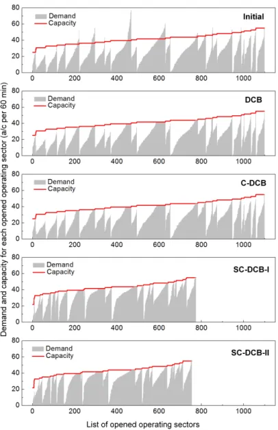
The demand and capacity situations are as shown in Fig. 7with respect to the initial case and those after executing the models. The x-axis of this figure represents a list of operating sectors, and each value corresponds to a specific operating sector, which is similar to a serial number. For each operating sector, we present its capacity (with the red curve) and also demand (with the grey bar) in Fig. 7.
We can see from the initial case that, across the 1,098 operating sectors in total, a certain amount of capacity overloads occur for some sectors. More-over, in some cases, the traffic demand could be more than double of the capacity. That is to say, for the purpose of balancing demand with capacity in Model DCB (see Fig. 7), we have to delay half of the flights traversing this
Figure 7: Demand and capacity situations (for each operating sector across the day) with respect to the initial case (i.e., pre-regulation) and the four models after execution (i.e., post-regulation).
sector, and the delayed flights will often incur new delays in other (near) con-gested sectors. This accumulative effect may easily evolve to large amount of total delays which we have seen in Table 4 for Model DCB.
to leverage the above delay accumulation, because diverting flights to some less-congested sectors does not necessarily generate new delays. As shown in Fig. 7, some free sectors with low traffic demand in Model DCB is now filled with higher demand. This can be seen more clearly by the capacity load shown in Fig. 8a, namely the blue line versus the red line. Worth noting that even with this slight improvement, the delays can be reduced remarkably (recall Table 4). Nevertheless, we may still see many blank areas in Model C-DCB underneath the capacity line, meaning that many capacities are not well utilised yet.
The proposed Model SC-DCB-I and SC-DCB-II solve this issue as well, as proved by the results in Fig. 7. The number of opened sectors are re-duced from 1,098 to 773 and 754 respectively, and all the traffic demand is compacted to the lessen area, which in turn leaves less blank areas unoccu-pied. Meanwhile, Fig. 8b presents the large improvement on capacity load for Model SC-DCB-I (green box) and for Model SC-DCB-II (pink box), if compared to the other two models. Finally, we may notice that not only the average capacity load increases, but also most of the sectors (75%) have their capacity loads greater than 60%. This number for Model DCB or C-DCB is only around 40%. On the other side, there appear almost 100 sectors in both Model DCB and C-DCB that have a capacity load less than 10% (with some 0% cases), which is fairly low, and sometimes is an unexpected situation from the safety aspect. In Model SC-DCB-I and SC-DCB-II, conversely, we may see only a few sectors having such low capacity loads.
5.4. Airspace configuration and sector opening
In Sec. 5.3, we have demonstrated that Model SC-DCB-I and SC-DCB-II enable a notable improvement on the utilisation of capacity resources. This is realised by optimising sector opening schemes and traffic flow (including assigning delays and alternative trajectories) in a harmonised way. Fig. 9a
shows the changes of number of opened sectors during each time period of the day, and we can observe the number reduction for every time period in Model SC-DCB-I (and even more reduction in Model SC-DCB-II).
Recall the objective function (15), where we minimise the total number of opened sectors. This is because less number of sectors leads to larger size for each of them, which means the demand could be further compacted (see Fig. 7) to reduce the percentage of “idle” capacity. However, the number of opened sectors cannot be reduced unlimitedly, as more traffic in less sectors will soon cause the capacities to be fully taken or even overloaded. Following
0 2 0 0 4 0 0 6 0 0 8 0 0 1 0 0 0 1 2 0 0 0 . 0 0 . 2 0 . 4 0 . 6 0 . 8 1 . 0 M o d e l D C B M o d e l C - D C B M o d e l S C - D C B - I M o d e l S C - D C B - I I C a p a c it y l o a d ( % ) O p e r a t i n g s e c t o r s
(a) Sorted capacity load
D C B C - D C B S C - D C B - I S C - D C B - I I - 2 0 0 2 0 4 0 6 0 8 0 1 0 0 1 2 0 D is tr ib u ti o n o f c a p a c it y l o a d ( % )
(b) Distribution of capacity load Figure 8: Final capacity load (i.e., demand and capacity ratio) in three models.
the reduced amount of operating sectors, the total capacity that the French ANSP needs to provide can be lowered down as well, as shown in Fig. 9b. Given that most sectors’ capacities are usually not varied significantly, the changes of capacity provisions are basically commensurate with the number of opened sectors.
Table 5: Airspace configurations’ opening scheme in Model SC-DCB-I for each ACC.
Time LFBBCTA LFEECTAC LFEECTAE LFEECTAN LFFFCTAA LFFFCTAE LFFFCTAW LFMLTMA LFMMCTAE LFMMCTAW LFMMXCTA LFRRCTAE LFRRCTAN LFRRCTAS LFSBTMA 1 1.A 1CA 1EB 1NB 1 1A 1A C1A E1A W1A CF1 C01EA C01NA C01SFS ALL 2 1.S 1CC 1EB 1NB 1 1A 1A C1A E1A W1A CF1 C01EFS C01NFS C01SA ALL 3 1.A 1CA 1EA 1NA 1 1A 1A C1A E1A W1A CF1 C01EFS C01NA C01SA ALL 4 1.S 1CB 1EA 1NA 1 1A 1A C1A E1A W1A CF1 C01EA C01NA C01SA ALL 5 1.A 1CB 1EC 1NA 1 1A 1A C1A E1A W1A CF1 C01EA C01NA C01SFS ALL 6 3.1AN 1CC 1EC 1NA 1 1A 1A C1A E1A W1A CF1 C01EA C01NFS C01SA ALL 7 9.1A 3CA 2EB 4NC 1 5C 2A C1A E4A W2A2A CF1 CO5EZZ C01NFS C01SA ALL 8 7.1D 2CA 2EB 5NA 1 3A 4C C1A E2B W2B1A CF1 C04EX C03NC C02SA ALL 9 14.1P 2CA 2EB 4NC 1 5C 3A C1A E4A W3B2A CF1 CO5EZZ C02NA C02SFS ALL 10 9.1D 3CA 2EB 5NA 1 4C 4A C1A E4A W2A2A CF1 C05EY C03NC C02SFS ALL 11 12.1G 3CA 2EB 4NC 1 5C 3A C1A E4B1A W4A1A CF1 C07EK C04NA C03SC ALL 12 12.1G 2CA 2EB 4NB 1 5F 3A C1A E4B1A W3B1A CF1 CO5EZZ C04NA C03SA ALL 13 12.1G 3CA 2EB 7NA 1 5F 4A C1A E4A W2A1A CF1 C07EG C03NC C02SA ALL 14 12.1G 2CA 2EB 5NN 1 3A 2A C1A E3C W3A1A CF1 C04EX C04NC C02SFS ALL 15 10.1E 3CA 2EB 5NA 1 5F 2A C1A E4E W3B2A CF1 C04EA C02NFS C03SA ALL 16 12.1G 2CA 2EB 5ND 1 4A 3A C1A E3C W2A1A CF1 CO5EZZ C02NA C02SA ALL 17 12.1G 2CA 2EB 4NC 1 3A 2A C1A E4A W3B1A CF1 C04EA C02NA C03SA ALL 18 14.1K 2CA 2EB 4NH 1 3A 2A C1A E3C W2A2A CF1 C07EE C02NA C03SC ALL 19 10.1E 2CA 2EB 4NH 1 4C 3B C1A E3C W2A1A CF1 C04EX C02NA C02SFS ALL 20 12.1G 2CA 1EB 4NB 1 3A 2A C1A E2B W2A2A CF1 C03EF C01NFS C02SFS ALL 21 12.1G 3CA 4EK 5NA 1 5F 4A C1A E2B W2A1A CF1 C05EX C02NA C02SA ALL 22 5.1D 1CC 1EB 1NB 1 1A 1A C1A E2B W2A1A CF1 C01EA C01NA C01SA ALL 23 1.A 1CC 1EA 1NB 1 1A 1A C1A E1A W1A CF1 C01EA C01NA C01SFS ALL 24 1.S 1CB 1EC 1NA 1 1A 1A C1A E1A W1A CF1 C01EFS C01NA C01SFS ALL
For the average capacity provision per opened sector (see Fig. 9c), the changes are worth noting. We can see that during the periods when there are less traffic (typically from 0-6 hour and 23-24 hour in a day), the initial setting provides a higher average capacity, whilst during the congested periods, it
2 4 6 8 1 0 1 2 1 4 1 6 1 8 2 0 2 2 2 4 0 1 0 2 0 3 0 4 0 5 0 6 0 7 0 8 0 9 0 1 0 0 N u m b e r o f o p e n e d s e c to rs ( # ) T i m e p e r i o d s ( h o u r ) I n i t i a l M o d e l S C - D C B - I M o d e l S C - D C B - I I
(a) Opened sectors
2 4 6 8 1 0 1 2 1 4 1 6 1 8 2 0 2 2 2 4 0 5 0 0 1 0 0 0 1 5 0 0 2 0 0 0 2 5 0 0 3 0 0 0 3 5 0 0 4 0 0 0 I n i t i a l M o d e l S C - D C B - I M o d e l S C - D C B - I I C a p a c it y p ro v is io n ( a /c ) T i m e p e r i o d s ( h o u r ) (b) Capacity provision 0 2 4 6 8 1 0 1 2 1 4 1 6 1 8 2 0 2 2 2 4 3 6 3 8 4 0 4 2 4 4 4 6 A v e ra g e c a p a c it y p ro v is io n ( a /c ) T i m e p e r i o d s ( h o u r ) I n i t i a l M o d e l S C - D C B - I M o d e l S C - D C B - I I
(c) Average capacity per opened sector
0 2 4 6 8 1 0 1 2 1 4 1 6 1 8 2 0 2 2 2 4 0 1 0 2 0 3 0 4 0 A v e ra g e d e m a n d ( a /c ) T i m e p e r i o d s ( h o u r ) I n i t i a l M o d e l S C - D C B - I M o d e l S C - D C B - I I
(d) Average demand per opened sector Figure 9: Changes of opened sectors in Model SC-DCB-I and Model SC-DCB-II.
somehow gives a relatively lower average value (see the grey line in Fig. 9c). This may be because the initial setting relies on cutting airspace into smaller pieces of sectors to better manage the traffic flow. On the contrary, Model SC-DCB-I and SC-SC-DCB-II provide an average capacity almost in consistent with the number of sectors and the capacity provisions (see the red and blue lines), meaning that the opened sectors share similar unit capacities. Moreover, the unit capacities are also higher than those of the smaller sectors used in the initial setting, and thus more demand is accommodated per sector.
above) from Model SC-DCB-I are presented. We can see that the choice of configuration, for the ACCs, evolves during different time periods of the day. As mentioned before, this model considers only a limited dynamic sectori-sation which is subject to the existing airspace configurations. For Model SC-DCB-II, however, the groups of collapsed and/or elementary sectors that are open in one time can be out of scope of the exiting configurations, which, in practice, may pose some non-negligible operational barriers such as devel-oping new ATC procedures.
5.5. Sensitivity analysis
Additional experiments have been conducted to explore the impacts of some key independent parameters, such as the flight delay cost and the cost of opening an operating sector (for a certain period of time). Specifically, the relationship of total capacity provision and traffic regulation has been also studied, producing a corresponding Pareto front to illustrate their trade-offs. The ranges of parameters in the sensitivity study are summarised in Table6. Note that, although the most promising findings have been tagged for Model SC-DCB-II, it does bring some future operational challenges such as the concept development of dynamic sectorisation. Therefore, the less ambitious yet more practical Model SC-DCB-I is used for the experimentation.
Table 6: Ranges of the independent parameters taken in the sensitivity study.
Parameters Min Max Step No.
Cost of delay (Euro/min) 5 50 5 10
Cost of sector opening (Euro/hr) 0 500 50 11
Maximal capacity provision (a/c) 32,000 37,000 500 11
The effects of having different flight delay costs are as shown in Figs. 10a,
10b and 10c, where the indicators in terms of delay (total delay and number of delayed flights), trajectory (number of flying the initial and alternatives), and airspace (capacity provision and number of opened sectors) are presented respectively. It can be noticed that the more expensive of undertaking one minute of delay, the less amount of system delay is assigned, which is then compensated by means of diverting more flights to the alternative trajectories and opening more sectors to supply more available capacities.
Similar to the effects observed when varying delay costs, the cost of open-ing an operatopen-ing sector (for a period of 60 min) has notable impacts on the
0 1 0 2 0 3 0 4 0 5 0 6 0 0 2 0 0 4 0 0 6 0 0 8 0 0 T o t a l d e l a y D e l a y e d f l i g h t C o s t o f d e l a y ( E u r o / m i n ) T o ta l d e la y ( m in ) 0 8 0 1 6 0 2 4 0 3 2 0 D e la y e d fl ig h ts ( a /c )
(a) Delay cost - Delay
0 1 0 2 0 3 0 4 0 5 0 6 0 5 7 0 0 5 7 2 0 5 7 4 0 5 7 6 0 5 7 8 0 I n i t i a l t r a j e c t o r y A l t e r n a t i v e t r a j e c t o r y C o s t o f d e l a y ( E u r o / m i n ) In it ia l tr a je c to ry ( a /c ) 4 8 0 4 9 5 5 1 0 5 2 5 5 4 0 A lte rn a tiv e tr a je c to ry ( a /c )
(b) Delay cost - Trajectory
0 1 0 2 0 3 0 4 0 5 0 6 0 3 2 4 0 0 3 3 0 0 0 3 3 6 0 0 3 4 2 0 0 3 4 8 0 0 C a p a c i t y S e c t o r C o s t o f d e l a y ( E u r o / m i n ) C a p a c it y p ro v is io n ( a /c ) 7 5 0 7 6 5 7 8 0 7 9 5 8 1 0 S e c to r o p e n in g ( # )
(c) Delay cost - Airspace
0 1 0 0 2 0 0 3 0 0 4 0 0 5 0 0 0 2 0 0 4 0 0 6 0 0 8 0 0 T o t a l d e l a y D e l a y e d f l i g h t C o s t o f o p e n i n g a s e c t o r ( E u r o ) T o ta l d e la y ( m in ) 0 8 0 1 6 0 2 4 0 3 2 0 D e la y e d fl ig h ts ( a /c )
(d) Sector cost - Delay
0 1 0 0 2 0 0 3 0 0 4 0 0 5 0 0 5 7 0 0 5 7 2 0 5 7 4 0 5 7 6 0 5 7 8 0 I n i t i a l t r a j e c t o r y A l t e r n a t i v e t r a j e c t o r y C o s t o f o p e n i n g a s e c t o r ( E u r o ) In it ia l tr a je c to ry ( a /c ) 4 8 0 4 9 5 5 1 0 5 2 5 5 4 0 A lte rn a tiv e tr a je c to ry ( a /c )
(e) Sector cost - Trajectory
0 1 0 0 2 0 0 3 0 0 4 0 0 5 0 0 3 1 2 0 0 3 2 4 0 0 3 3 6 0 0 3 4 8 0 0 C a p a c i t y S e c t o r C o s t o f o p e n i n g a s e c t o r ( E u r o ) C a p a c it y p ro v is io n ( a /c ) 7 2 0 7 5 0 7 8 0 8 1 0 S e c to r o p e n in g ( # )
(f) Sector cost - Airspace
3 2 0 0 0 3 3 0 0 0 3 4 0 0 0 3 5 0 0 0 3 6 0 0 0 3 7 0 0 0 0 2 0 0 4 0 0 6 0 0 8 0 0 T o t a l d e l a y D e l a y e d f l i g h t M a x i m u m c a p a c i t y a l l o w a n c e ( a / c ) T o ta l d e la y ( m in ) 0 8 0 1 6 0 2 4 0 3 2 0 D e la y e d fl ig h ts ( a /c ) (g) Capacity - Delay 3 2 0 0 0 3 3 0 0 0 3 4 0 0 0 3 5 0 0 0 3 6 0 0 0 3 7 0 0 0 5 7 0 0 5 7 2 0 5 7 4 0 5 7 6 0 5 7 8 0 I n i t i a l t r a j e c t o r y A l t e r n a t i v e t r a j e c t o r y M a x i m u m c a p a c i t y a l l o w a n c e ( a / c ) In it ia l tr a je c to ry ( a /c ) 4 8 0 4 9 5 5 1 0 5 2 5 5 4 0 A lte rn a tiv e tr a je c to ry ( a /c ) (h) Capacity - Trajectory 3 2 0 0 0 3 3 0 0 0 3 4 0 0 0 3 5 0 0 0 3 6 0 0 0 3 7 0 0 0 3 1 5 0 0 3 3 0 0 0 3 4 5 0 0 3 6 0 0 0 3 7 5 0 0 C a p a c i t y S e c t o r M a x i m u m c a p a c i t y a l l o w a n c e ( a / c ) C a p a c it y p ro v is io n ( a /c ) 7 0 0 7 5 0 8 0 0 8 5 0 9 0 0 S e c to r o p e n in g ( # )
(i) Capacity - Airspace Figure 10: Sensitivity analysis of key independent parameters (including cost of delay, cost of opening an operating sector, and the maximal total capacity provision) with respect to the main output (in terms of delay, trajectory and airspace) of the model.
main indicators too. Fig. 10d shows a positive relation between the amount of delay (and delayed flights) with the sector opening cost, whilst the opposite situation occurs for the amount of flights maintaining their initial trajectories (see Fig. 10e), as well as the total capacity provision and sector openings as can be appreciated from Fig. 10f.
In terms of the trade-off between capacity provision and delay assign-ment given in Fig. 10g, obviously the more capacities it can make use of, the less number of delay will be required. However, such decrease is not linear which turns slower to eventually zero when redundant capacities are avail-able, meaning that the efficiency of delay reduction will decline if the system
is constantly added with more capacities. For the trajectory selection, the same situation applies as shown in Fig. 10h, being the amount of flights who can still use their initial trajectories not increased once the total capacity is reaching some point (i.e., around 33,000 in this case). Finally, the relation be-tween the actual capacity provided (which is determined by certain airspace configurations) versus the maximum capacity that is allowed is presented in Fig. 10i. A slight decline can be seen within the linear increasing segment at higher levels of capacities, which means that these redundant capacities are not necessarily utilised (because of the low efficiency in reducing the delay and trajectory related costs).
6. Conclusions
In this paper, we demonstrated an approach with collaborative ATFM strategy, so as to realise synchronised demand and capacity balancing, by means of optimising both traffic flows and airspace configurations. The traf-fic regulation initiatives (e.g., assigning ground holding and using alterna-tive trajectories) and a dynamic opening scheme for airspace configuration (or sectorisation) method were incorporated into a centralised optimisation model. Comparing the results from the relevant four model variants solving the same ATFM problem, we showed some notable benefits with the pro-posed approach. In particular, the AUs delays can be largely reduced, along with the reduced ANSP operational costs and total capacity provisions. The main findings of this framework aimed at the European airspace align with the recent research conducted in the United States National Airspace System with respect to CTOP and DAC. However, there are still significant opera-tional barriers for the work toward a workable solution, and we envision that some follow-up research could be enlightened for overcoming such barriers in the near future.
As for the significance of each component to the final performance of the framework, we may conclude that allowing the alternative trajectory options could reduce the required AUs delay notably. Meanwhile, synchronising the airspace adjustment, whether in terms of configurations or sectorisations, could further reduce the delay, but more importantly contribute to reducing the number of opened sectors. Nevertheless, as shown with the work flow presented in Fig. 2, all the components are linked as a whole and there are so many aspects that could affect the final performance, which we believe deserves a thorough assessment in our future work. Also, it is envisaged
that the model should be further enhanced with increased robustness to take the uncertainty factors into account through implementing stochastic programming.
Acknowledgment
The work presented in this paper was partially funded by the SESAR Joint Undertaking under grant agreement No 699338, as part of the European Unions Horizon 2020 research and innovation programme: APACHE project (Assessment of Performance in current ATM operations and of new Con-cepts of operations for its Holistic Enhancement - http://apache-sesar. barcelonatech-upc.eu/en). The opinions expressed herein reflect the au-thors view only. Under no circumstances shall the SESAR Joint Undertaking be responsible for any use that may be made of the information contained herein. The authors would also like to thank Mr. Ramon Dalmau from the Technical University of Catalonia for generating the relevant trajectory data.
References
Ball, M. O., Hoffman, R. L., Knorr, D., 2000. Assessing the benefits of col-laborative decision making in air traffic management. In: Proceedings of the 3rd USA/Europe ATM R&D Seminar. Napoli, Italy.
Bertsimas, D., Lulli, G., Odoni, A., 2011. An integer optimization approach to large-scale air traffic flow management. Operations research 59 (1), 211– 227.
Bertsimas, D., Patterson, S. S., 1998. The air traffic flow management prob-lem with enroute capacities. Operations research 46 (3), 406–422.
CAAC, 2016. Statistics of key performance indicators for China’s civil avia-tion industry, Civil Aviaavia-tion Administraavia-tion of China.
Dalmau, R., Melgosa, M., Vilardaga, S., Prats, X., 2018. A fast and flexible aircraft trajectory predictor and optimiser for atm research applications. In: Proceedings of the 8th International Conference for Research in Air Transportation (ICRAT). Castelldefels, Spain.
Delahaye, D., Alliot, J.-M., Schoenauer, M., Farges, J.-L., 1994. Genetic algorithms for partitioning air space. In: Proceedings of the 10th Confer-ence on Artificial IntelligConfer-ence for Applications. IEEE, San Antonia, US, pp. 291–297.
Delahaye, D., Schoenauer, M., Alliot, J.-M., 1998. Airspace sectoring by evolutionary computation. In: Proceedings of 1998 IEEE International Conference on Evolutionary Computation. IEEE, Anchorage, USA, pp. 218–223.
Eurocontrol, 2017. All-causes delay and cancellations to air transport in Eu-rope. Tech. Rep. CODA Digest 2016, CDA-2017-005, Network Manager. FAA, 2002. National airspace redesign strategic management plan. Tech. Rep.
Revision 3b, Federal Aviation Administration.
FAA, 2009. Traffic Flow Management in the National Airspace System. Tech. Rep. FAA-2009-AJN-251, Federal Aviation Administration.
FAA, 2014. Collaborative Trajectory Options Program (CTOP): Document Information. Tech. Rep. AC 90-115, Federal Aviation Administration. Gianazza, D., 2007. Airspace configuration using air traffic complexity
metric. In: Proceedings of the 7th USA/Europe ATM R&D Seminar. Barcelona, Spain.
Klein, A., Rodgers, M. D., Kaing, H., 2008. Dynamic FPAs: A new method for dynamic airspace configuration. In: Proceedings of 2008 Integrated Communications, Navigation and Surveillance Conference (ICNS). IEEE, Bethesda, US, pp. 1–11.
Kopardekar, P., Bilimoria, K., Sridhar, B., 2007. Initial concepts for dynamic airspace configuration. In: Proceedings of the 7th AIAA Aviation Tech-nology, Integration and Operations Conference (ATIO). AIAA, Belfast, Northern Ireland.
Libby, M., Buckner, J., Brennan, M., 2005. Operational concept for Airspace Flow Programs (AFP). Tech. rep., FAA Air Traffic Organization, Systems Operations Services.
Lulli, G., Odoni, A., 2007. The European air traffic flow management prob-lem. Transportation Science 41 (4), 431–443.
Melgosa, M., Prats, X., Xu, Y., Delgado, L., 2019. Alternative trajectory options and traffic volume based hotspot detection for advanced demand and capacity balancing. In: 38th IEEE/AIAA Digital Avionics Systems Conference (DASC). IEEE, San Diego, California, US.
Miller, M. E., Hall, W. D., 2015. Collaborative trajectory option program demonstration. In: Proceedings of the 34th IEEE/AIAA Digital Avionics Systems Conference (DASC). IEEE, Prague, Czech Republic, pp. 1C1–8. Odoni, A. R., 1987. The flow management problem in air traffic control.
In: Flow control of congested networks. Springer, Berlin, Heidelberg, pp. 269–288.
SESAR, 2015. Step 1 v3 UDPP validation report, optimised airspace user operations. Tech. Rep. PJ07.06.02, SESAR JU.
Sherali, H. D., Hill, J. M., 2013. Configuration of airspace sectors for balanc-ing air traffic controller workload. Annals of Operations Research 203 (1), 3–31.
Terrab, M., Paulose, S., 1992. Dynamic strategic and tactical air traffic flow control. In: IEEE International Conference on Systems, Man and Cyber-netics. IEEE, Chicago, US, pp. 243–248.
US Department of Transportation, 2016. Airline on-time statistics. Tech. rep. URL https://www.transtats.bts.gov/
Xu, Y., Dalmau, R., Melgosa, M., de Montlaur, A., Prats, X., 2018. Alter-native trajectories for delay reduction in demand and capacity balancing. In: Proceedings of the 8th International Conference for Research in Air Transportation (ICRAT). Castelldefels, Spain.
Xu, Y., Prats, X., 2017. Including linear holding in air traffic flow manage-ment for flexible delay handling. Journal of Air Transportation 25, 123–137.