Fully Dynamic Consistent Facility Location
Vincent Cohen-Addad, CNRS & Sorbonne Universit´e
[email protected] Niklas Hjuler, University of Copenhagen [email protected] Nikos Parotsidis, University of Copenhagen [email protected] David Saulpic, Ecole normale sup´erieure
Sorbonne Univerist´e [email protected]
Chris Schwiegelshohn Sapienza University of Rome [email protected]
Abstract
We consider classic clustering problems in fully dynamic data streams, where data elements can be both inserted and deleted. In this context, there are several important parameters: (1) the quality of the solution after each insertion or deletion, (2) the time it takes to update the solution, and (3) how different consecutive solutions are. The question of obtaining efficient algorithms in this context for facility location,k-median andk-means has been raised in a recent paper by Hubert-Chan et al. [WWW’18] and also appears as a natural follow-up on the online model with recourse studied by Lattanzi and Vassilvitskii [ICML’17] (i.e.: in insertion-only streams).
In this paper, we focus on general metric spaces and mainly on the facility location problem. We give an arguably simple algorithm that maintains a constant factor approximation, withO(nlogn)update time, and total recourseO(n). This im-proves over the naive algorithm which consists in recomputing a solution after each update and that can take up toO(n2)update time, andO(n2)total recourse. Our bounds are nearly optimal: in general metric space, inserting a point takesO(n)
times to describe the distances to other points, and we give a simple lower bound ofO(n)for the recourse. Moreover, we generalize this result for thek-medians andk-means problems: our algorithms maintain a constant factor approximation inOe(n+k2)time per update.
We complement our analysis with experiments showing that the cost of the solution maintained by our algorithm at any timetis very close to the cost of a solution obtained by quickly recomputing a solution from scratch at timetwhile having a much better running time.
1
Introduction
Clustering is a core procedure in unsupervised machine learning and data analysis. Due to the large number of applications, clustering problems have been extensively studied for several decades. The existing literature includes both very precise algorithms[1,18,31], and very fast ones [34]. Due to the importance of the task, clustering problems have also been studied in several computing settings, such as the streaming model [11] and the sliding-window model [7], the distributed model [4], in the dynamic model [24], and others.
Applications nowadays operate on dynamically evolving data, e.g., pictures are constantly added and deleted from picture repositories, purchases are continuously added into online shopping systems, reviews are added or being edited in retail systems, etc. Due to the scale and the dynamic nature
of the data at hand, conventional algorithms designed to operate on static inputs become unable to handle the task for two main reasons. First, the running time of even the most efficient algorithms is too expensive to execute after every single change in the input data. Second, re-running a static algorithm after every update might generate solutions that differ substantially between consecutive updates, which might be undesirable for the application at hand. The number of changes in the maintained solution between consecutive updates is called therecourseof the algorithm. Our study is motivated by these limitations of static algorithms, or dynamic algorithms that are effective on only one of the two objectives.
Most fundamental problems in computer science have been studied in the dynamic setting. In a very high-level, a dynamic algorithm computes a solution on the initial input data and as the input undergoes insertions or/and deletions of elements, the algorithm updates the solution to reflect the current state of the data. A dynamic algorithm may allow only insertions or only deletions, or may support an intermixed sequence of insertions and deletions, in which case the algorithm is called fully dynamic. The running time of a dynamic algorithm can either guarantee a worst-case update time after each update, or a bound on the average update time over a sequence of updates which is called amortized update bound. A dynamic algorithm with worst-case update bounds is the most desirable, and often hard to obtain, but in several applications algorithms with amortized update bounds are sufficient.
Most of the clustering-related literature has focused on the online model where the updates are restricted to insertions only and a decision cannot be revoked or on the streaming model where there is a specific memory budget not to be exceeded. However, as observed by Lattanzi and Vassilvitskii [30] the online model may appear too restrictive: if a bad decision has been made, it is often fine to spend some time to correct it instead of suffering the bad decision (i.e.: keeping a bad clustering) for the rest of the stream. However, spending too much time on the modification of the clustering may be counterproductive and that’s what we aim at capturing in the fully-dynamic model with limited recourse: keeping a good clustering by spending the least among of time and making as few changes to the current clustering as possible.
In this paper, we study fully-dynamic algorithms for classic clustering problems. In particular, we consider the facility location, thek-means, and thek-median problems in the dynamic setting. In the static case, these problems are defined as follows. LetXbe a set ofnpoints, andd:X×X →R a distance function. We assume thatdis symmetric and that(X, d)forms a metric space. For the(k, p)-clustering problem, the objective function that we seek to optimize is Cp(X, S), where S⊆X,|S|=k. Settingp= 1gives thek-median objective, andp= 2thek-means one. For the facility location problem the objective function is C(X, S).
C(X, S) := X x∈X min c∈Sd(x, c) +f· |S| Cp(X, S) := X x∈X min c∈Sd p(x, c),
All of these problems are NP-Hard, so our best hope is to design algorithms with provable approxi-mation guarantees. There is an extensive line of work on algorithms with constant approxiapproxi-mation guarantees for all three aforementioned problems [1,3,10,20,26,27,31,33]. On the other hand, Mettu and Plaxton [34] showed anΩ(nk)lower bound for computing anO(1)-approximate solution for k-median and k-means in general metric spaces.
In the dynamic setting, the goal is to maintain efficiently a good solution to the clustering problem at hand as the set of points undergoes element insertions and deletions. The main criterion for designing a
gooddynamic algorithm for these problems is the quality of the clustering, with respect to the optimum solution, at any given time. However, in many applications, it is equally important to maintain a
consistentclustering, namely a clustering with bounded recourse. Lattanzi and Vassilvitskii [30] have recently considered consistent clustering problems in the online setting, where the points appear in sequence and the objective is to maintain a constant factor approximate solution while minimizing the total number of times the maintained solution changes over the whole sequence of points. Another criterion that has been explored much less but which is highly important when dealing with massive data is the time it takes to update the solution after each update so that the solution remains within a constant factor from the optimum solution.
1.1 Our Contribution
We present the first work that studies fully-dynamic algorithms while considering the approximation guarantee, consistency and update time, all at the same time. From an input perspective, we consider general metric spaces. Thus, an element of the input is a point in a metric space which is defined by the distances to the other points of the metric. The contribution of our paper is summarized as follows:
•We give a fully-dynamic algorithm for the facility location problem that maintains a constant factor approximate solution with constant recourse per update andO(nlogn)update time. We moreover show that constant recourse per update is necessary for achieving a constant factor approximation.
•We extend the algorithm for facility location to thek-median andk-means problems. Here, our algorithm maintains a constant factor approximate solution withOe(n+k2)1update time (Theo-rem3.1). This is the first non-trivial result for these problems, as the only known solution for these problems was to recompute from scratch after each update: this requires timeΩ(nk)fork-median andΩ(n2)for facility location, per update. Hence, our time bounds are significantly better than the naive approach for a large range ofk.
Empirical Analysis. We complement our study with an experimental analysis of our algorithm on three real-world data sets and show that it outperforms the standard approach that recomputes a solution from scratch after each update using a fast static algorithm. Interestingly, we show that this barely impacts the approximation guarantee. At the same time, our algorithm outperforms by at least three orders of magnitude the simple-minded solutions, both in terms of running time and total number of changes made in the maintained solution throughout the update sequence.
1.2 Related Work
Online and Consistent Clustering. Online algorithms for facility location were first proposed by Meyerson [35] in his seminal paper. Fotakis [16] later showed that the algorithm has a competitive ratio of O(logn/log logn), which is also optimal. Additionally, the algorithm has a constant competitive ratio if the points arrive in a random order [35,29]. There also existO(logn)competitive deterministic algorithms, see [2,15]. This was recently extended to the online model that incorporates deletions [12].
Online algorithms for clustering that are only allowed to place centers cannot be competitive. This led to the consideration of the incremental model, which allows two clusters to be merged at any given time. Work in this area includes [9,14]. The number of reassignments (commonly referred to asrecourse) over the execution of an incremental algorithm may be arbitrary. However, recently, Lattanzi and Vassilvitskii [30] considered the online clustering problem with bounded total recourse. They showed a lower bound ofΩ(klogn)changes over an arbitrary sequence of updates, and presented an algorithm that can maintain a constant factor approximation while limiting the total recourse toO(k2·log4n)
. Their work differs to ours in that elements can only be added, and that they do not consider optimizing the running time. In the fully dynamic case their bound on the recourse does not hold, and we moreover show that constant recourse per update is unavoidable.
Fully-Dynamic and Streaming Algorithms. Streaming algorithms for clustering can be used to obtain fast dynamic algorithms by recomputing a clustering after each update. Since streaming algorithms are highly memory compressed and typically process updates in time linear in the memory requirement, the approach automatically yields good update times. Low-memory adaptations of Meyerson’s algorithm [35] turned out to be simple and particularly popular, see [8,29,37]. Another technique for designing clustering algorithms in the streaming models is by maintaining coresets, see the following recent survey for an overview [36]. For fully dynamic data streams, the only known algorithms for maintaining coresets fork-means andk-median in Euclidean spaces using small space and update times are due to Braverman et al. [6] and Frahling and Sohler [17]. There also exists some work on estimating the cost of Euclidean facility location in dynamic data streams, see [13,25,28]. For more general metrics, the problem of maintaining a clustering dynamically has been considered by Henzinger et al. [22] and Goranci et al. [19] who consider the facility location in bounded doubling
1
e
dimension. The arguably most similar previous work to ours is due to Hubert-Chan et al. [24]. They consider thek-center problem in general metrics in the fully dynamic model. Here, they were able to maintain a constant factor approximation with update timeO(klogn)2. Whether an algorithm in the fully dynamic model with low recourse and update times exists, was left as an open problem. 1.3 Preliminaries
We assume that we are given some finite metric space (X, d), whereX is the set of points and d:X×X →R≥0a distance function. Every entryd(a, b)is stored in a (symmetric)n×nmatrix D. Our algorithms work in the distance oracle model, which assumes that we can access any entry of Din constant time.
Our input consists of tuples(X,Rn≥0,{−1,1}). The first coordinate is the identifier of some point p∈X, the second coordinate is the column/row vector inDassociated withp, and the last coordinate signifies insertion(1)or deletion(−1). We assume that the stream is consistent, which means that no point can be deleted without having been previously inserted. The adversary generating the point sequence is called adaptive if he can modify the sequence depending on the algorithm’s choices. Throughout the paper, we letXtbe the set of points present at timet,nbe the total number of updates, andn∗:= supt∈1,...,n|Xt|be the maximum number of points present at the same time. We
denote byOP Ttthe optimum solution at timet. All our results could be phrased in term of|Xt|,
but for simplicity we present them in terms ofn∗.
Roadmap. Our paper is organized as follows. In Section2, we describe our algorithm for fully dynamic facility location. Section3extends these results tok-median andk-means clustering. We conclude with an experimental evaluation of our algorithms in Section4on real-world benchmarks. All omitted proofs can be found in the supplementary material.
2
Dynamic Facility Location
The goal of this section is to prove the following theorem.
Theorem 2.1. There exist a randomized algorithm that, given a metric space undergoing insertion and deletions of points, maintains a set of centerStsuch that :
• each update is processed in timeO(n∗log (n∗))with probability1−1/n∗
• at any given timet, C(Xt, St) =O(1)·C(Xt,OPTt)
with probability1−1/n∗
• Pn t=0|S
t4St+1|=O(n), i.e. the amortized recourse isO(1)per update.
The proof is divided into several lemmas: we first study how the optimal cost behaves upon dynamic updates, and we exhibit then an algorithm that maintains a solution whose cost evolves in a similar way as the optimum.
Although, perhaps counter intuitive, removing a point from the input in a finite metric may increase the cost of a clustering, if one cannot locate a center there anymore. We show in the supplementary material that this increase is bounded by a factor 2: this leads to the following lemma, which bounds the evolution of the optimal cost.
Lemma 2.2. Let OPTbef ore be the optimal cost of an initial metric spaceX. After an arbitrary
sequence ofniinsertions andnddeletions of points inX, the optimal solution OPTaf tersatisfies
OPTbef ore/2−nd·f ≤OPTaf ter≤2(OPTbef ore+ni·f)
Maintaining a solution during a few updates.We now turn on designing an algorithm competitive with the optimal solution, showing first how to deal with a small number of updates. In order to process deletions, we define the notion ofsubstitutecenters: given a functionsmapping every center from the initial solution to a center in the current one, we say thats(c)substitutesc. Initially,s(c) =c. When a centercis deleted, the algorithm opens a replacement centercr, and updates the functions:
s(s−1(c)) =c
r.
2
Under the common assumption that the ratio longest distance / shortest distance of the metric is polynomially bounded.
The algorithm is as follows: when a pointxis inserted, we open as a facility atx, and for convenience we defines(x) =x. When a pointxis deleted, we have two cases: eitherxwas not an open facility, in which case the algorithm does nothing, orxwas a facility. In the latter case, letc=s−1(x): the algorithm opens the closest pointc0ofcinX0that is still part of the metric, and sets(c) =c0. This choice ofc0ensures that, for all pointsxin the current metric space,d(c0, c)≤d(x, c).
Lemma 2.3. Starting from any metric space(X0, d)and anα-approximation with costΘ, the algorithm described above maintains a(8α+ 4)-approximation during 4Θαf updates, withO(1)
recourse andO(n∗)time amortized per update.
Proof. This algorithm opens at most one new facility at every update: the recourse is thus at most 1. The time to process an insertion is constant, and the time to process a deletion is at mostO(n∗)(the time required to compute the closest point tox).
We now analyse the cost of the solution produced aftertupdates. Since the recourse is at most 1 per update, the cost of open facilities increases by at mostt·f. Since every inserted points is opened as a center, it does not contribute to the connection cost: this cost changes therefore only by deletions of points fromX0. Similarly to Lemma2.2, one can show that the connection cost of a pointx∈X0 at most doubles. More formally, letc∈X0be the center that servesxin the initial solution. Let c0 = s(c)be the center that substitutesc in the current metric. By the choice ofc0 and triangle inequality, it holds thatd(x, c0)≤d(x, c) +d(c, c0)≤2d(x, c). Hence, the total serving cost is at
most twice as expensive as in the initial solution. The cost at timetis therefore at most2Θ +t·f. Lett≤ Θ
4αf, and OPT
0the optimal cost in the initial state. By Lemma2.2, the optimal cost at timet is at least OPT0/2−t·f ≥OPT0/4, since by definition ofαit holdst≤OPT0
4f . Moreover, the cost
of our algorithm at timetis at mostΘ(2 +α1)≤OPT0(2α+ 1). Combining the two inequalities gives that our algorithm is a(8α+ 4)-approximation for allt≤ Θ
4αf, which concludes the proof.
We remark that the parameters can be optimized: for instance, with a suitable data structure, the time to find a substitute center can be logarithmic; however, this is dominated by the complexity of finding the initialα-approximation.
Maintaining a solution for any number of updates.We combine Lemma2.3with a classic static O(1)-approximation algorithm, namely Meyerson’s algorithm, to prove Theorem2.1.
Proof of Theorem2.1. We summarize here the useful properties of Meyerson algorithm, and refer to the supplementary material for more details. The algorithm processes the input points in a random order, opening each pointxwith probabilityd(x, F)/f(whereF is the set of previously opened facilities). If the algorithm openskfacilities, its running time isO(kn∗), and the cost is at least
Θ≥kf. Hence, the running time isO(Θ/f·n∗). Moreover, one can assume that the cost is always at mostn∗f (by opening a facility at every point).
We say that a run of Meyerson’s algorithm isgoodif it yields aO(1)-approximate solution. By the analysis in [35], a run is good in expectation (where the randomness comes from the random ordering of points): hence, by runninglog(2n∗)independent copies of the algorithm, at least one run is good with probability1−(1/n∗)2. We letαbe the approximation constant of this algorithm.
Therefore, our main algorithm works as follows: start with a solution given by Meyerson’s algorithm of costΘ, use Lemma2.3to maintain a solution during 4Θαf updates, and then recompute from scratch. We call the intervals between consecutive recomputationsperiods, and note that they are random objects: the length of a period is determined by the cost of its initial solution, which is a random variable.
We first analyze the running time of this algorithm. Within one period, Lemma2.3ensures that the running time isO(n∗)per update. Moreover, the running time of the initial recomputation is O(Θ/f·n∗logn∗), and the length of the period isΩ(Θ/f). Therefore the amortized running time is
e
O(n∗)per update. Since the initial recourse isO(Θ/f), the same argument proves that the recourse is amortizedO(1)per update.
We aim at using again Lemma2.3to prove that, at a given timet, the solution is a constant factor approximation. For this, letPbe the period in whichtappears. If the period is good, then Lemma2.3
concludes. Unfortunately, the fact thattis inP is not independent ofP being good (for instance, if Pis very long it is unlikely to be good). However, note that the starting time ofPcannot be before t−n∗: indeed, a period lasts for at most 4Θαf ≤n∗f
4αf ≤n
∗updates. Hence, if we condition on all
periods starting betweent−n∗andt, Lemma2.3applies and the solution at timetis a constant factor approximation. Since any period is good with probability1−(1/n∗)2, all periods between t−n∗andtare good with probability1−1/n∗by union bound. This concludes the proof. The algorithm sketched in the previous proof can be transformed so that the complexity becomes
e
O(n∗)in the worst case, by spreading the recomputation over several updates (see supplementary material). Moreover, randomization is not needed in order to maintain the solution (only to compute a starting approximation): hence the algorithm works against an adaptive adversary.
We conclude this section by showing that our algorithm is (up to a logarithmic factors) optimal both for update time and recourse.
Proposition 2.4. Any algorithm maintaining aO(1)-approximation for Facility Location must have an amortized update timeΩ(n∗)and total recourseΩ(n), wherenthe total number of updates.
3
Dynamic
k
-Median and
k
-Means in Linear Time
In this section we adapt the algorithm from Section2to handle the stricter problems ofk-Median and k-Means. For simplicity, we call(k, p)-clustering the problem of findingkcenters that minimize Cp
(p= 1fork-Median andp= 2fork-Means).
Roughly speaking, our algorithm works as follows. We use an adaptation of the algorithm from Section2to maintain a coresetRofOe(k)points that contain a constant factor approximate solution for the(k, p)-clustering problem. Then, we apply a constant factor approximation algorithm for the metric(k, p)-clustering problem on the maintained coreset (e.g., we can use a quadratic-time local-search algorithm, see [21]). This yields the following theorem.
Theorem 3.1. There exists a randomized algorithm that, given a metric space undergoing insertions and deletions of points, maintains a set of centersStwith
e
O(n∗+k2)update time such that, for any
timet, Cp(Xt, St) =O(1)·Cp(Xt,OPTt).3
The remainder of this section is devoted in proving Theorem3.1. The main hurdle in applying the framework from Section2is that the optimum solution can change drastically with the addition or deletion of a point, and it is therefore not easy to adapt the previous amortization argument. To overcome this barrier, we make use of the following lemma, from [9] and [30]:
Lemma 3.2. LetLbe some integer. With probability1/2, running Meyerson’s algorithm for Facility Location withf = k(1+logL n∗) gives a setSof4k·(1 + logn∗)·(2
2p+1·Cp(X,OPT)
L + 1)centers
such that Cp(X, S)≤L+ 4·Cp(X,OPT).
For completeness, we provide the pseudocode of Meyerson’s algorithm, adapted for our purpose, in ProcedureM eyersonCapped. The lemma implies that, if we know a valueLthat approximates OPT within a factor2, ProcedureM eyersonCappedcomputes a set of pointsRand an assignment of pointsφsuch thatP
x∈Xd(x, φ(x))≤6·Cp(X,OPT)with probability1/2. This probability can
be boosted to1−(1/n∗)2by taking the union ofq=O(logn∗)independent copies of the algorithm. Therefore for alli= 1, ..., q, our algorithm will use this lemma assuming Cp(X,OPT)∈[2i,2i+1), and takingL= 2i. This provides, for alli, a setR
iofO(klog2n∗)centers.
It remains to maintain those sets dynamically. Similarly to Section2, we use the solution computed by ProcedureM eyersonCappedfor the subsequentkupdates, so that we can amortize the update-time bound. However, for(k, p)-clustering it is not possible to bound the cost of OPT after a few updates. We overcome this obstacle by updating the setsRimore carefully. More precisely, letRt
i be the
(updated) setRiaftertupdates of the algorithm. The algorithm ensures the following invariant:
Invariant 3.3. The setRt
ihas sizeO(klog
2n∗)and, with high probability, there existsisuch that
Cp(Xt,Rti) =O(1)·Cp(Xt,OPTt).
3
We assume (as in [30]) that the minimum distance in the metric is1and the maximum∆is bounded by a polynomial inn∗. Alternatively, our bounds can be stated withlog ∆instead oflogn∗.
Input: An integerL, a set of pointsX
Output: A set of centersR, an assignmentφ of point to centers, andtlthe id of the last
center opened
1: Let R ← ∅and x1, ..., x|X| be a random
order on the points ofX 2: for alli∈ {1, ...,|X|}do
3: if|R| <4k·(1 + logn∗)·(22p+2+ 1) then
4: add xi to R with probability
d(xi,R)pk(1+logn) L 5: if|R|= 4k·(1 + logn∗)·(22p+2+ 1) then 6: tl←i 7: end if 8: end if 9: φ(xi)←arg min c∈R {d(xi, c)p} 10: end for (a) MeyersonCapped(L, X)
Input: IntegersLandtl, a set of pointsX and
a set of centersR
Output: UpdatedRandtl, an assignmentφof
points to centers
1: {tlis the last timeM eyersonCappedwas
invoked.}
2: for allj∈ {tl, ...,|X|}do
3: ifno center was opened yetthen
4: add xj to R with probability
d(xj,R)pk(1+logn∗) L 5: ifxjis added toRthen 6: tl←j,φ(xj)←xj 7: end if 8: else{Updateφ} 9: φ(xj)← arg min z∈{φ(xj),xtl} {d(xj, z)p} 10: end if 11: end for
(b) DeletePoint(L, tl, X,R). L is the value with
which we approximate Cp(X,OPT)andtlis the last
time MeyersonCapped opened a center.
For this, initializeRito be the union of the outputs ofq=O(logn∗)independent executions of M eyersonCapped(Li, X), forLi= 2iandi= 1, ..., q. The algorithm updates these sets duringk
updates before recomputing them from scratch. In the case of a point insertion, it suffices to add the new point to allRi: overkupdates, this changes the cardinality by at mostkwhile the cost remains the same, and therefore the two conditions are met. The case of a point deletion requires more work. The idea is, as in Section2, to replace the deleted center by its closest point. However, this is not enough to ensure Invariant3.3: this is taken care of by ProcedureDeleteP oint, which finds the next point inXtthatM eyersonCappedwould open, if there was no constraint on the size ofR.
We are now ready to describe our fully-dynamic algorithm for maintaining a constant-approximate solution to the(k, p)-clustering problem. The algorithm uses ProceduresM eyersonCappedand DeleteP ointas subroutines to build and maintain the setsRifori, and after each update calls the static constant-approximate algorithm to compute an approximate solutionSti on each weighted instanceRi (where the weight of each pointx∈ Ricorresponds to the number of points ofXt
assigned toxby the functionφi, computed in ProceduresM eyersonCappedandDeleteP oint.
After each update, the algorithm keeps the solutionSt
i that minimizes Cp(Rti, Sit), that is,St=Sit
fori= arg mini{Cp(Rti, Sit)}. The pseudocode of the algorithm is stated in Algorithm1. The proof
of Invariant3.3is stated in the supplementary material. The next lemma, together with Invariant3.3, shows thatStcan be used as a solution for the entire setXt.
Lemma 3.4. Let OPT(Rt
i)be the optimal solution in the weighted set Rti. Then it holds that
Cp(Xt,OPT(Rit))≤23p−1(Cp(X,Rti) +Cp(Xt,OPTt)).
This proves the second part of Theorem3.1: forisuch that Cp(Xt,Rt
i) =O(1)·Cp(Xt,OPT t), the
solution computed on the setRt
iis a good approximation of the optimal solution, and therefore the
algorithm maintains a constant factor approximation. The bound on the running time being similar to the one of Section2, we provide it in the supplementary material.
4
Empirical Analysis
In this section, we evaluate our algorithm for facility location experimentally. Recall that we aim to strike a balance between (1) overall running time, (2) the cost of the solution, (3) the total recourse. Our implementation follows the framework outline in Theorem2.1. As part of the recomputation step between two periods, we run 5 independent executions of Meyerson’s algorithm, and selecting the execution with lowest cost. The updates within a period are handled by assigning to closest center if distance is less thanf or otherwise open a new center at the point, and we simply remove a client if it gets deleted. We compare our algorithm against two variants of Meyerson’s algorithm.
Algorithm 1Fully Dynamic(k, p)-clustering Input: For allt,Xtbe the set of points at timet
Output: For allt, a setStof centers at timetand an mappingφt:Xt→Stof points toSt 1: LetRt
i be the coreset at timetforLi, andφti the function mapping every point ofXtto its
closest point inRt i
2: Lett0be the last timeM eyersonCappedwas called 3: for alltimetdo
4: ifa pointxtis insertedthen
5: LetRt i=R
t−1
i ∪ {xt},∀i∈[logn]
6: else ifa pointxtis removedthen 7: for alli←1, ...,logndo 8: ifxt∈ R/ t−1
i then
9: Rt← Rt−1
10: else
11: Letz←φt0(xt)
12: Letz0 ∈Xtbe the closest toz (breaking ties arbitrarily) 13: Rt← Rt−1∪ {z0}
14: {tilis the last timeM eyersonCapped was invoked onRt−1}
15: CallDeleteP oint(Li, til,Rt−1)
16: end if
17: end for 18: end if
19: iftis a multiple ofkthen
20: {Recompute from scratch allRi}
21: t0←t
22: for alli←1, ...,logndo
23: Rt
i ←M eyersonCapped(Li, Xt)
24: end for 25: end if
26: {Keep the best among allRt iand assignmentsφt} 27: (i, St)← arg min i,Ci=A(Rti) Cp(Ci,Rti) 28: Letψ:Rt i→Cibe the assignment computed byA 29: φt←ψ◦φti 30: end for
The first one, termedMeyersonRec, re-runs Meyerson at every single update. The second, termed
MeyersonSingle, consists of a single execution of Meyerson for all updates, where deletions are handled by just removing the distance cost of the deleted point. Following Hubert-Chan et al. [24], we incorporate deletions by considering a sliding window over the data set. A point is inserted/deleted when it enters/exists the window, respectively.
Data Set and Setup. We consider the following data sets, equipped with the Euclidean distance.
• The Twitter data set [23], considered by [24], consists of 4.5 million geotagged tweets in 3
dimensions (longitude, latitude, timestamp). We restricted our experiments to the first 200K tweets.
•The COVERTYPE data set [5], considered by [30], from the UCI repository with 581K points and 54 dimensions. We restricted our experiments to the first 100K points and 10 dimensions (the ones we believed to be appropriate for an Euclidan metric).
•The USCensus1990 data set [32] from the UCI repository has 69 dimensions and 2.5 million points. We restricted our experiments to the first 30K points.
We restricted the number of points considered due to time constraints. Since larger data sets typically have more complicated ground truths, we used a larger windows for them containing more samples. To avoid overfitting, we also adjusted the cost of opening a facility depending on the window size, i.e. for larger windows a lower opening cost per facility. For COVERTYPE and USCensus1990, we used a window size of 5000 points and a facility cost of0.5; for Twitter, the window size was 10000 and the facility cost0.004. All our codes are written in Python. The experiments were executed on a Windows 10 machine with processor: Intel(R) Core(TM) i7-8700K CPU @ 3.70GHz, 3701 Mhz, 6 cores, 12 Logical processors, and 16 GB RAM.
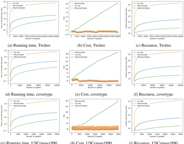
Results. In all three data sets we generally observed the same behavior in terms of running time, cost, and the number of clusters opened, see Figure2. Our algorithm is 100 times faster than MeyersonRec. Compared to MeyersonSingle, our algorithm is slower initially. When the number of processed points becomes very large, the running time of MeyersonSingle deteriorates comparatively, as it never removes a facility once it has been opened: the time to compute the distance to the
(a) Running time, Twitter. (b) Cost, Twitter. (c) Recourse, Twitter.
(d) Running time, covertype. (e) Cost, covertype. (f) Recourse, covertype.
(g) Running time, USCensus1990. (h) Cost, USCensus1990. (i) Recourse, USCensus1990. Figure 2: A comparison of the algorithms we consider in terms of running time (left column), cost of the solution (middle column), and recourse (right column).
set of facilities is therefore increasing (see Figure 1 in the supplementary material). The cost of MeyersonSingle generally has a linear dependency on the number of updates, though the slope is very gentle. This is also what our algorithm takes advantage off, broadly speaking by approximating the curve with a step function (adapted to handle insertions and deletions). The cost of our algorithm and MeyersonRec is basically indistinguishable, and in certain cases our algorithm fares even slightly better. The recourse of our algorithm is expectedly much better than MeyersonRec by a wide margin, and significantly worse than MeyersonSingle.
Finally, we ran our algorithm with multiple choices of facility costf, and we observed that the recourse is almost independent of the both cost and running time of the algorithm, and only depends on the number of updates. This is consistent with tracking evolving data in time, where the underlying ground truth clustering also evolves in time.
Acknowledgements. Nikos Parotsidis is supported by Grant Number 16582, Basic Algorithms Research Copenhagen (BARC), from the VILLUM Foundation. Ce projet a b´en´efici´e d’une aide de l’ ´Etat g´er´ee par l’Agence Nationale de la Recherche au titre du Programme FOCAL portant la r´ef´erence suivante : ANR-18-CE40-0004-01.
References
[1] S. Ahmadian, A. Norouzi-Fard, O. Svensson, and J. Ward. Better guarantees for k-means and euclidean k-median by primal-dual algorithms. In2017 IEEE 58th Annual Symposium on Foundations of Computer Science (FOCS), pages 61–72, Oct 2017.
[2] A. Anagnostopoulos, R. Bent, E. Upfal, and P. V. Hentenryck. A simple and deterministic competitive algorithm for online facility location.Inf. Comput., 194(2):175–202, 2004.
[3] V. Arya, N. Garg, R. Khandekar, A. Meyerson, K. Munagala, and V. Pandit. Local search heuristics for k-median and facility location problems. SIAM J. Comput., 33(3):544–562, 2004. [4] O. Bachem, M. Lucic, and A. Krause. Distributed and provably good seedings for k-means in
constant rounds. InProceedings of the 34th International Conference on Machine Learning (ICML), pages 292–300, 2017.
[5] J. A. Blackard, D. J. Dean, and C. W. Anderson. Covertype data set,https://archive.ics. uci.edu/ml/datasets/covertype.
[6] V. Braverman, G. Frahling, H. Lang, C. Sohler, and L. F. Yang. Clustering high dimensional dynamic data streams. In Proceedings of the 34th International Conference on Machine Learning (ICML), pages 576–585, 2017.
[7] V. Braverman, H. Lang, K. Levin, and M. Monemizadeh. Clustering problems on sliding windows. InProceedings of the Twenty-Seventh Annual ACM-SIAM Symposium on Discrete algorithms (SODA), pages 1374–1390, 2016.
[8] V. Braverman, A. Meyerson, R. Ostrovsky, A. Roytman, M. Shindler, and B. Tagiku. Streaming k-means on well-clusterable data. InProceedings of the Twenty-Second Annual ACM-SIAM Symposium on Discrete Algorithms (SODA), pages 26–40, 2011.
[9] M. Charikar, C. Chekuri, T. Feder, and R. Motwani. Incremental clustering and dynamic information retrieval. SIAM J. Comput., 33(6):1417–1440, 2004.
[10] M. Charikar and S. Guha. Improved combinatorial algorithms for the facility location and k-median problems. In40th Annual Symposium on Foundations of Computer Science, (FOCS), pages 378–388, 1999.
[11] M. Charikar, L. O’Callaghan, and R. Panigrahy. Better streaming algorithms for clustering problems. InProceedings of the Thirty-fifth Annual ACM Symposium on Theory of Computing (STOC), pages 30–39, 2003.
[12] M. Cygan, A. Czumaj, M. Mucha, and P. Sankowski. Online facility location with deletions. In
26th Annual European Symposium on Algorithms (ESA), pages 21:1–21:15, 2018.
[13] A. Czumaj, C. Lammersen, M. Monemizadeh, and C. Sohler. (1+)-approximation for facility location in data streams. InProceedings of the Twenty-Fourth Annual ACM-SIAM Symposium on Discrete Algorithms (SODA), pages 1710–1728, 2013.
[14] D. Fotakis. Incremental algorithms for facility location andk-median. Theor. Comput. Sci., 361(2-3):275–313, 2006.
[15] D. Fotakis. A primal-dual algorithm for online non-uniform facility location. J. Discrete Algorithms, 5(1):141–148, 2007.
[16] D. Fotakis. On the competitive ratio for online facility location. Algorithmica, 50(1):1–57, 2008.
[17] G. Frahling and C. Sohler. Coresets in dynamic geometric data streams. InProceedings of the 37th Annual ACM Symposium on Theory of Computing (STOC), pages 209–217, 2005. [18] T. F. Gonzalez. Clustering to minimize the maximum intercluster distance. Theoretical
Computer Science, 38:293 – 306, 1985.
[19] G. Goranci, M. Henzinger, and D. Leniowski. A tree structure for dynamic facility location. In
26th Annual European Symposium on Algorithms (ESA), pages 39:1–39:13, 2018.
[20] S. Guha and S. Khuller. Greedy strikes back: Improved facility location algorithms. J. Algorithms, 31(1):228–248, 1999.
[21] A. Gupta and K. Tangwongsan. Simpler analyses of local search algorithms for facility location.
[22] M. Henzinger, D. Leniowski, and C. Mathieu. Dynamic clustering to minimize the sum of radii. In25th Annual European Symposium on Algorithms (ESA), pages 48:1–48:10, 2017.
[23] T. Hubert Chan, A. Guerqin, and M. Sozio. Twitter data set, https://github.com/ fe6Bc5R4JvLkFkSeExHM/k-center.
[24] T. Hubert Chan, A. Guerqin, and M. Sozio. Fully dynamick-center clustering. InProceedings of the 2018 World Wide Web Conference on World Wide Web (WWW), pages 579–587, 2018. [25] P. Indyk. Algorithms for dynamic geometric problems over data streams. InProceedings of the
36th Annual ACM Symposium on Theory of Computing (STOC), pages 373–380, 2004. [26] K. Jain and V. V. Vazirani. Approximation algorithms for metric facility location andk-median
problems using the primal-dual schema and lagrangian relaxation. J. ACM, 48(2):274–296, 2001.
[27] T. Kanungo, D. M. Mount, N. S. Netanyahu, C. D. Piatko, R. Silverman, and A. Y. Wu. A local search approximation algorithm for k-means clustering.Comput. Geom., 28(2-3):89–112, 2004. [28] C. Lammersen and C. Sohler. Facility location in dynamic geometric data streams. In
Proceed-ings of the 16th Annual European Symposium (ESA), pages 660–671, 2008.
[29] H. Lang. Online facility location against at-bounded adversary. InProceedings of the Twenty-Ninth Annual ACM-SIAM Symposium on Discrete Algorithms (SODA), pages 1002–1014, 2018. [30] S. Lattanzi and S. Vassilvitskii. Consistent k-clustering. InProceedings of the 34th International
Conference on Machine Learning (ICML), pages 1975–1984, 2017.
[31] S. Li. A 1.488 approximation algorithm for the uncapacitated facility location problem. Infor-mation and Computation, 222:45 – 58, 2013.
[32] C. Meek, B. Thiesson, and D. Heckerman. Us census data (1990),http://archive.ics. uci.edu/ml/datasets/US+Census+Data+(1990).
[33] R. R. Mettu and C. G. Plaxton. The online median problem. SIAM J. Comput., 32(3):816–832, 2003.
[34] R. R. Mettu and C. G. Plaxton. Optimal time bounds for approximate clustering. Machine Learning, 56(1):35–60, Jul 2004.
[35] A. Meyerson. Online facility location. In42nd Annual Symposium on Foundations of Computer Science (FOCS), pages 426–431, 2001.
[36] A. Munteanu and C. Schwiegelshohn. Coresets-methods and history: A theoreticians design pattern for approximation and streaming algorithms. KI, 32(1):37–53, 2018.
[37] M. Shindler, A. Wong, and A. Meyerson. Fast and accurate k-means for large datasets. In
Proceeding of the Twenty-fifth Conference on Neural Information Processing Systems (NIPS), pages 2375–2383, 2011.