Scalable Embeddings for
Kernel Clustering on MapReduce
byAhmed Elgohary
A thesis
presented to the University of Waterloo in fulfillment of the
thesis requirement for the degree of Master of Applied Science
in
Electrical and Computer Engineering
Waterloo, Ontario, Canada, 2014
I hereby declare that I am the sole author of this thesis. This is a true copy of the thesis, including any required final revisions, as accepted by my examiners.
Abstract
There is an increasing demand from businesses and industries to make the best use of their data. Clustering is a powerful tool for discovering natural groupings in data. Thek-means al-gorithm is the most commonly-used data clustering method, having gained popularity for its effectiveness on various data sets and ease of implementation on different computing architec-tures. It assumes, however, that data are available in an attribute-value format, and that each data instance can be represented as a vector in a feature space where the algorithm can be ap-plied. These assumptions are impractical for real data, and they hinder the use of complex data structures in real-world clustering applications.
The kernel k-means is an effective method for data clustering which extends the k-means algorithm to work on a similarity matrix over complex data structures. The kernel k-means al-gorithm is however computationally very complex as it requires the complete data matrix to be calculated and stored. Further, the kernelized nature of the kernelk-means algorithm hinders the parallelization of its computations on modern infrastructures for distributed computing. This the-sis defines a family of kernel-based low-dimensional embeddings that allows for scaling kernel k-means on MapReduce via an efficient and unified parallelization strategy. Then, three practical methods for low-dimensional embedding that adhere to our definition of the embedding family are proposed. Combining the proposed parallelization strategy with any of the three embedding methods constitutes a complete scalable and efficient MapReduce algorithm for kernelk-means. The efficiency and the scalability of the presented algorithms are demonstrated analytically and empirically.
Acknowledgements
Thanks to everyone who directly or indirectly helped me to complete this thesis at this quality. I would like to give a special mention to:
• My professors at Alexandria University, Prof. Noha Yousri, Prof. Mohamed Ismail, and Prof. Moustafa Youssef, for guiding my first research endeavours, for being great examples for work ethics, and for encouraging and helping me to join the University of Waterloo. • My supervisors, Prof. Fakhri Karray and Prof. Mohamed Kamel, for the great opportunity
they offered me to join the University of Waterloo, and for the freedom and trust they gave to me throughout the program.
• Mostafa Hassan for his precious advices in my first days at Waterloo.
• Waterloo professors, Prof. Ashraf Aboulnaga, Prof. Paul Marriott, and Prof. Ali Ghodsi, for their great courses that were my most valuable assist in producing this thesis.
• Ahmed Farahat for guiding me in learning about several background fundamentals, for closely mentoring all of my thesis research, and for his technical and non-technical advices. • Radha Chitta for sharing her processed ImageNet data set that I used throughout all my
experiments.
• Mike Miao for his feedback and suggestions on this work, and for presenting parts of this thesis at NIPS.
Dedication
Table of Contents
List of Tables ix List of Figures x List of Algorithms xi 1 Introduction 1 1.1 Motivation. . . 1 1.2 Summary of Contributions . . . 3 1.3 Thesis Organization . . . 3 1.4 Notations . . . 42 Background and Related Work 5 2.1 MapReduce Framework. . . 5
2.2 Data Clustering . . . 6
2.3 Kernel Methods . . . 7
2.4 Kernel Approximations . . . 9
2.4.1 The Nystr¨om Approximation . . . 9
2.4.2 Random Fourier Features. . . 10
2.5 Kernel-Based Clustering . . . 11
2.5.2 Spectral Clustering . . . 13
2.5.3 Equivalence of Kernelk-Means and Spectral Clustering . . . 14
2.6 Related Work . . . 14
2.6.1 Kernelk-Means Approximations. . . 14
2.6.2 Distributed Data Clustering . . . 15
2.6.3 MapReduce for Kernel Clustering . . . 16
3 Scaling Kernelk-Means on MapReduce 17 3.1 Approximate Nearest Centroid Embeddings . . . 17
3.2 Efficient MapReduce-Based Parallelization Strategy . . . 19
3.2.1 APNC Embedding on MapReduce . . . 20
3.2.2 APNC Clustering on MapReduce . . . 21
3.3 APNC Embedding via Nystr¨om Method . . . 22
3.4 APNC Embedding via Ensemble Nystr¨om Method . . . 24
3.5 APNC Embedding via Stable Distributions . . . 27
3.6 Analysis . . . 31
3.7 Implementation Details . . . 33
3.7.1 Deterministic versus Probabilistic Sampling . . . 33
3.7.2 Handling Empty Clusters . . . 34
3.7.3 Convergence and Local Optima . . . 35
3.7.4 Clustering Output . . . 36
4 Experiments and Results 37 4.1 Single Node Experiments . . . 38
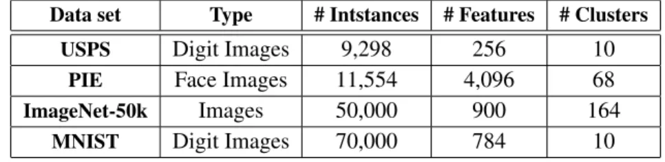
4.1.1 Datasets . . . 38
4.1.2 Setup . . . 38
4.1.3 Results . . . 42
4.2.1 Datasets . . . 42
4.2.2 Setup . . . 46
4.2.3 Results . . . 53
5 Conclusions and Future Work 55
5.1 Conclusions . . . 55
5.2 Future Work . . . 56
List of Tables
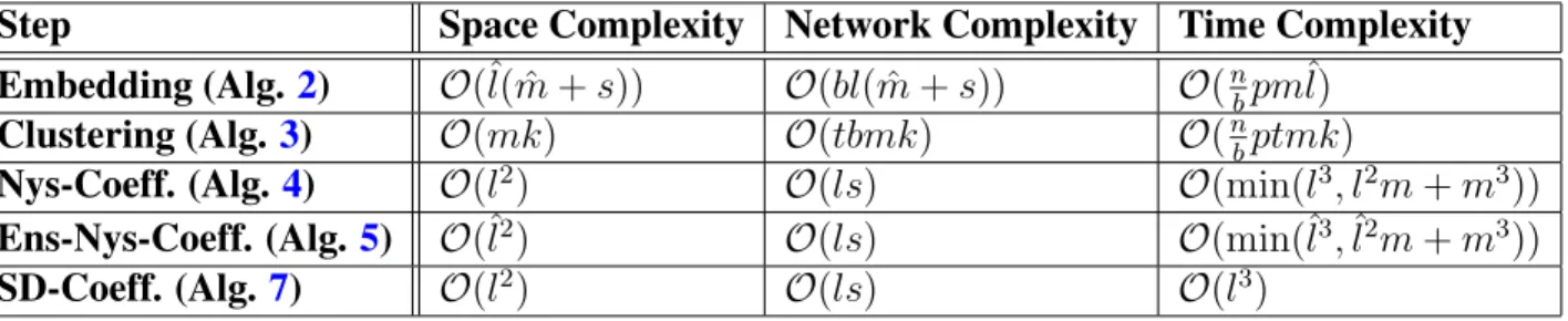
3.1 The space, time, and network communication complexities of the steps of the proposed approach. . . 33
4.1 The properties of the datasets used in the single-node experiments. . . 38
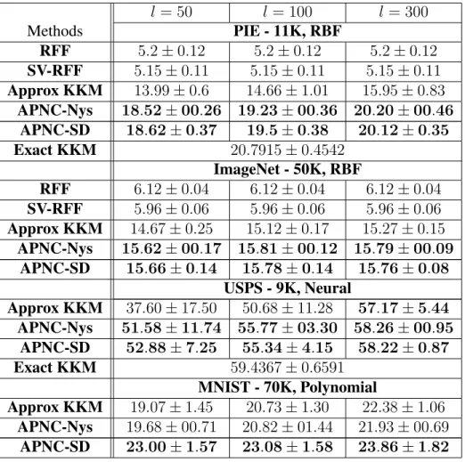
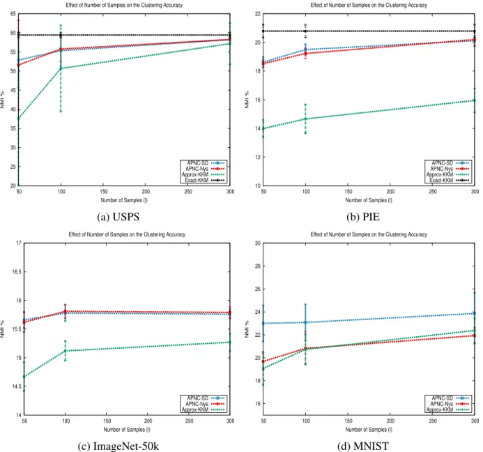
4.2 The NMIs (%) of different kernelk-means approximations (single-node experi-ments). In each sub-table, the best performing approximation(s) for eachl, (ac-cording tot-test with95%confidence level) is highlighted in bold. . . 40
4.3 The properties of the data sets used in the large-scale experiments. . . 45
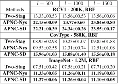
4.4 The NMIs (%) of different kernel k-means approximations (large-scale experi-ments). In each sub-table, the best performing approximation(s) for eachl, (ac-cording tot-test with95%confidence level) is highlighted in bold. . . 47
4.5 The clustering times in minutes of differentAPNC-NysandAPNC-SD. For each dataset, the faster method according tot-test (with95%confidence level) is high-lighted in bold. . . 49
List of Figures
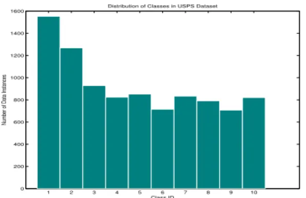
4.1 Number of data instances per class in the USPS dataset . . . 39
4.2 Number of data instances per class in the ImageNet-50k dataset . . . 39
4.3 Clustering accuracy of kernelk-means approximations using different numbers of samplesl . . . 41
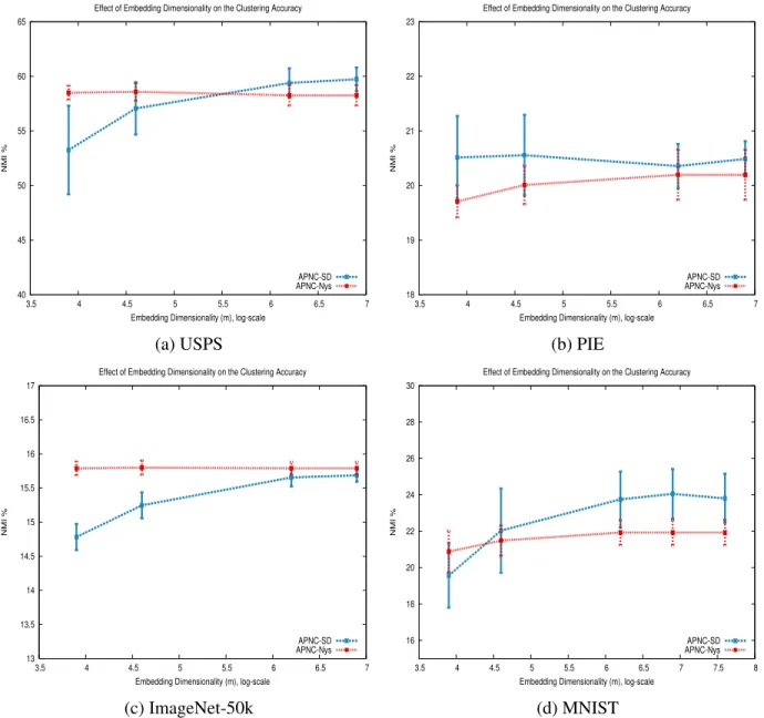
4.4 Clustering accuracy of APNC embeddings (APNC-SD and APNC-Nys) using different values for the target dimensionalitym . . . 43
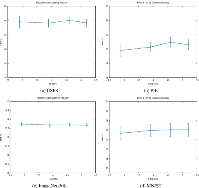
4.5 Clustering accuracy of APNC embeddings via Stable Distributions (APNC-SD) using different values for the Gaussianity parametert . . . 44
4.6 Number of data instances per class in the RCV1 dataset . . . 45
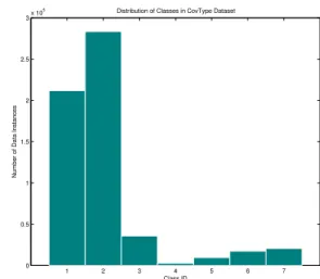
4.7 Number of data instances per class in the CovType dataset . . . 45
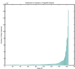
4.8 Number of data instances per class in the ImageNet dataset . . . 46
4.9 Embedding time of APNC embeddings via Nystr¨om method (APNC-Nys) and APNC embeddings via stable distributions (APNC-SD) using different sample sizeslin different datasets . . . 48
4.10 Embedding time of APNC embeddings via Nystr¨om method (APNC-Nys) and APNC embeddings via stable distributions (APNC-SD) using different dataset sizes . . . 49
4.11 The linear scalability of APNC embeddings . . . 50
4.12 Clustering time of APNC embeddings via Nystr¨om method (APNC-Nys) and APNC embeddings via stable distributions (APNC-SD) using different dataset sizes . . . 50
4.14 The embedding time of APNC embeddings using different values for the embed-ding dimensionality (m). . . 51
4.15 The clustering time of APNC embeddings using different values for the embed-ding dimensionality (m). . . 52
4.16 The NMIs (%) of APNC embeddings using different values for the embedding dimensionality (m) . . . 52
List of Algorithms
1 Lloydk-means . . . 7
2 APNC Embedding on MapReduce . . . 20
3 APNC Clustering on MapReduce. . . 22
4 APNC Coefficients via Nystr¨om Method . . . 23
5 APNC Coefficients via Ensemble Nystr¨om Method . . . 27
6 Approximate Kernelk-Means Using Stable Distributions . . . 29
7 APNC Coefficients via Stable Distributions . . . 30
8 Deterministic Subset Sampling . . . 33
9 Handling Empty Clusters in APNC Clustering . . . 34
Chapter 1
Introduction
1.1
Motivation
In today’s era of big data, there is an increasing demand from businesses and industries to get an edge over competitors by making the best use of their data. Clustering is one of the powerful tools that data scientists can employ to discover natural groupings in data. Thek-means algorithm [1] is the most commonly-used data clustering method. It has gained popularity for its effectiveness on many data sets as well as the ease of its implementation on different computing architectures. Thek-means algorithm, however, assumes that data are available in an attribute-value format, and that all attributes can be turned into numeric values so that each data instance is represented as a point or vector in some feature space where the algorithm can be applied. These assumptions are impractical for real data and they hinder the utilization of complex data structures in real-world clustering problems. Examples include grouping users in a social network based on their friendship networks, clustering customers according to their behaviour, and grouping proteins based on their structures. Data scientists tend to simplify these complex structures to a vectorized format, and would accordingly lose the richness of the data they have.
In order to overcome this problem, much research has been conducted on clustering algo-rithms that work on similarity matrices over data instances, rather than on a vector representation of the data in a feature space. This has led to the advance of different similarity-based methods for data clustering, such as kernel k-means [2] and spectral clustering [3]. The focus of this thesis is on the kernelk-means algorithm [2]. Different from the traditionalk-means algorithm, the kernelk-means algorithm works on kernel matrices which encode different aspects of sim-ilarity between complex data structures [4]. It has also been shown that the widely-accepted spectral clustering method has an objective function which is equivalent to a weighted variant
of the kernel k-means algorithm [2], which means that optimizing that criterion allows for an efficient implementation of the spectral clustering algorithm, in which computationally complex eigendecomposition step is bypassed [5]. Accordingly, the methods proposed in this thesis can be leveraged for scaling the spectral clustering method on MapReduce.
The kernelk-means algorithm, however, depends on calculating and storing the kernel matrix over all data instances. Further, all entries of the kernel matrix need to be accessed in each iteration. As a result, the kernelk-means algorithm has quadratic space and time complexities per iteration. These complexities become scalability bottlenecks as the dataset size increases. Some recent work [6,7] has been proposed to approximate the kernelk-means clustering, and allow its application to large data. However, those algorithms are designed for centralized settings, and assume that the data will fit on the memory/disk of a single machine.
This thesis proposes a family of algorithms for scaling the kernelk-means over cloud infras-tructures for distributed computing. Such infrasinfras-tructures tend to be composed of several com-modity nodes, each of which is of a limited memory and computing power [8–10]. The nodes are connected together in a shared-nothing cluster, which means that data transfers between different nodes are done through the network. In such settings, ensuring the scalability and fault tolerance of data analysis tasks is troublesome. MapReduce [9] is a programming model, supported by an execution framework that provides scalable and fault-tolerant execution of analytical data pro-cessing tasks over distributed infrastructures of commodity nodes. The proposed algorithms in this thesis are designed to perfectly fit into the MapReduce programming model, and to adhere to its computational constraints. We also optimize the execution of the proposed algorithms by considering the different performance aspects of the target computing infrastructure.
Our approach is based on eliminating the scalability bottlenecks of the kernel k-means by first learning an embedding of the data instances, and then using this embedding to approximate the cluster assignment step in each iteration of the kernelk-means algorithm. We show that this approach leads to a unified and MapReduce-efficient scaling strategy. In addition, we generalize our approach by defining a family of embeddings characterized by only four properties, which ensure the correctness of any embedding method in the defined family for scaling the kernel k-means on MapReduce.
1.2
Summary of Contributions
The contributions of the thesis can be summarized as follows.
• The thesis proposes a generic family of kernelized low-dimensional embeddings, which is called Approximate Nearest Centroid (APNC) embeddings, and defines its computational and statistical properties that facilitate scaling kernelk-means on MapReduce.
• Exploiting the properties of APNC embeddings, the thesis presents a unified and efficient parallelization strategy on MapReduce for approximating the kernel k-means using any APNC embedding.
• The thesis proposes three practical instances of APNC embeddings which are based on the Nystr¨om method and the use ofp-stable distributions for approximating vector norms.
• The presented algorithms are analyzed in terms of their space, time, and network commu-nication complexities. These analytical results are used to prove the efficiency and the the scalability of the proposed approach.
• Extensive medium and large-scale experiments were conducted to compare the proposed approach to state-of-the-art kernelk-means approximations, and to demonstrate the effec-tiveness and scalability of the presented algorithms.
1.3
Thesis Organization
The rest of this chapter describes the notations used throughout the thesis. The first part of Chap-ter 2 gives an introductory background on data clusChap-tering, kernel methods, and cloud analytics using MapReduce, while the second part discusses related work on scaling kernel-based cluster-ing methods, and the recent efforts at adoptcluster-ing data anlytics tasks on MapReduce. The proposed approach and algorithms are given in Chapter 3. The experiments conducted, and their results, are described in Chapter 4. Finally, the conclusion of the thesis, and a set of possible future extensions are presented in Chapter 5.
1.4
Notations
The following notations are used throughout the thesis unless otherwise indicated. Scalars are denoted by small letters (e.g.,m,n), sets are denoted in script letters (e.g.,L), vectors are denoted by small bold italic letters (e.g.,φ,y), and matrices are denoted by capital letters (e.g.,Φ,Y). In addition, the following notations are used:
For a setL:
L(b) the subset ofLcorresponding to the data blockb. |L| the cardinality of the set.
For a vectorx∈Rm:
xi i-th element ofx. x(i) thei-th vector.
x[b] the vectorxcorresponding to the data blockb. kxkp the`p-norm ofx.
For a matrixA ∈Rm×n:
Aij (i, j)-th entry ofA.
Ai: i-th row ofA. A:j j-th column ofA.
AL:,A:L the sub-matrices ofAwhich consist of the setLof rows and columns respectively. AT the transpose ofA.
Chapter 2
Background and Related Work
2.1
MapReduce Framework
Distributed cloud computing infrastructures tend to be composed of several commodity nodes, each of which is of a limited memory and computing power [8–10]. The nodes are connected together in a shared-nothing cluster which, means that data transfers between different nodes are done through the network. In such settings of infrastructure, ensuring the scalability and fault tolerance of data analysis tasks is troublesome. MapReduce [9] is a programming model supported by an execution framework that provides scalable and fault tolerant execution of ana-lytical data processing tasks over distributed infrastructures of commodity nodes. The simplicity of the MapReduce API, together with its scalable and fault-tolerant execution framework, dis-tinguished MapReduce and its open-source implementation Hadoop [11] as the most attractive paradigm for data analytics tasks on large-scale cloud computing infrastructures.
The rationale behind MapReduce is to impose a set of constraints on data access at each node and communication between different nodes, to ensure both the scalability and fault-tolerance of the analytical tasks. A MapReduce job is executed in two phases of user-defined data transfor-mation functions, namely, themapandreducephases. The input data is split into physical blocks distributed across the nodes, each block is viewed as a list of key-value pairs. In the first phase, the key-value pairs of each input block b are processed by a singlemapfunction, running inde-pendently on the node where the block b is stored. The key-value pairs are provided one-by-one to themapfunction; the output of themapfunction is another set of intermediate key-value pairs. The values associated with the same key across all nodes are grouped together and provided as an input to the reduce function in the second phase. Different groups of values are processed in parallel on different machines. The output of each reducefunction is a third set of key-value
pairs, and collectively considered the output of the job. For complex analytical tasks, multiple jobs are typically chained together [12], and/or many rounds of the same job are executed on the input data set [13].
It is important to note that in addition to the processing time of themapandreducefunctions, a major portion of the job execution time is that taken to move the intermediate key-value pairs across the network. Hence, minimizing the size of the intermediate key-value pairs significantly reduces the overall running time of MapReduce jobs. Further, since the individual nodes in cloud computing infrastructures are of very limited memory, a scalable MapReduce-algorithm should ensure that the memory required per node remains within the bound of commodity memory sizes as the data size increases. A significant amount of research has been devoted for scaling complex data analytics algorithms on MapReduce by developing efficient parallelization strategies, or even by introducing novel approximations that lead to MapReduce-efficient algorithms. Such algorithms spanned text mining [14], graph mining [15,16], nonnegative matrix factorization [17], feature selection [18], regression [19], PageRank [20] and most recently column subset selection [12].
2.2
Data Clustering
Data clustering is an unsupervised learning task that aims at discovering natural grouping in unlabelled input datasets. Over the past decades, researchers have developed various application-specific [21,22] or general-purpose [23,24] data clustering approaches. Data clustering has been used in a wide spectrum of applications, ranging from news organization [20] to indoor localization [25].
Thek-means algorithm [1] is the most widely used algorithm for data clustering. The objec-tive of the algorithm is to group the data points intokclusters, such that the Euclidean distances between data points in each cluster and that cluster’s centroid are minimized. LetPcdenote the
set of data instances assigned to the clustercandx¯(c)denote the centroid of the data instances in Pc(i.e.x¯(c)= nc1 Pi∈Pcx
(i)) wheren
c=|Pc|. Thek-means objective is to assign the input data
points tokdisjoint setsPcforc= 1,2, . . . , k such that following loss function is minimized:
Loss= k X c=1 X i∈Pc x(i)−x¯(c) 2 2 . (2.1)
An iterative algorithm, namely Lloyd’s algorithm [26], is usually used for the optimization of the loss function in 2.1. In each iteration, Lloyd’s algorithm assigns each data point to the
Algorithm 1Lloydk-means
Input:DatasetX ={x(1), x(2), . . . , x(n)}, Number of clustersk Output:kclustersP1,P2, . . . ,Pk
1: Generate initialkcentroidsx¯(1),x¯(2), . . . ,x¯(k)
2: repeatuntil convergence
3: Reset all cluster setsPc← {}, forc= 1, . . . , k
4: fori= 1 :n 5: ˆc←arg minc x(i)−x¯(c) 2 2 6: Pˆc← Pˆc∪x(i) 7: end
8: Update cluster centroids asx¯(c) = 1
nc P
x∈Pcx, forc= 1, . . . , k
9: end
nearest centroid, and calculates new centroids based on the current assignment of the data points. Afterwards, cluster centroids are updated based on the new cluster assignments. Algorithm 1
outlines the steps of Lloyd’s algorithm. The algorithm is known to converge to a local-optimal solution. In addition, it can be observed from the steps of algorithm1 that data instances are required to be represented in a vector form. Further, the k-means objective in general forces the clusters to be separated by a hyperplane [5], which makes thek-means unable to discover non-linearly separable clusters.
2.3
Kernel Methods
One appealing idea for dealing with data of non-linear structures is to use a mapping (embedding) function to map each data instancexto a typically high-dimensional feature space (asφ=ϕ(x)) in which data instances become linearly separable. Applying a linear learning algorithm (e.g. k-means) to the data instances in the new feature space provides an elegant replacement for developing non-linear algorithms and applying them directly to non-linearly separable data in their original form. However, mapping each data instance to the new feature space might be intractable, or a computationally expensive step. Further, to obtain the desired linear-separability properties, the new feature space is usually extremely high dimensional (possibly of infinite dimensionality) and accordingly, working with the explicit mappingsφis most often infeasible.
Mercer’s theorem [27] was the key result that enabled researchers to put the idea of mapping data instances to high-dimensional spaces into a computationally tractable framework, known as
kernel methods [4]. Mercer’s theorem indicates that a symmetric function (a kernel)κ(., .)can be expressed as an inner productedκ(x(i), x(j)) = ϕ(x(i))Tϕ(x(j))for some mapping functionϕif and only ifκ(., .)is positive semi-definite. That is, the matrix whose entries are [κ(x(i), x(j))]
i,j
is positive semi-definite for any set X = {x(1), x(2), . . . , x(n)}. According to that theorem, if each data access step of a linear learning algorithm is expressed as an inner product of a pair of instances, one will no longer need to explicitly compute each mappingϕ(x(i)). Instead, each inner productϕ(x(i))Tϕ(x(j))can be substituted with the output of the kernel function between the two corresponding original data instancesκ(x(i), x(j)). Throughout this thesis, for an input datasetX = {x(1), x(2), . . . , x(n)}, we refer to the matrix[κ(x(i), x(j))]
i,j as thekernel matrix.
The new feature space endowed by a kernel function is referred to as thekernel space.
The idea of kernel methods have been applied to several machine learning algorithms. The most popular example of such an algorithm is the support vector machines [4]. Commonly used kernel functions that have been employed successfully in various learning tasks are (1) the Radial Basis Function (RBF) kernel, which is given by:
κ(x(i), x(j)) = exp − x(i)−x(j) 2 2σ2 ! ,
whereσ is a tuning parameter known as the kernel width; (2) the Polynomial kernel, which is given by: κ(x(i), x(j)) = x(i)Tx(j)+ 1 d ,
wheredis a tuning parameter that determines the polynomial degree; and (3) the Sigmoid kernel, which is given by κ(x(i), x(j)) =tanh ax(i)Tx(j)+b ,
where bothaandbare tuning parameters.
Kernel methods have also been shown to be useful for handling datasets of complex structures [28]. Examples of such data structures are text strings, graphs, and biological sequences. Since most learning algorithms work on data points represented in a vector space, data scientists had to simplify these complex structures to a vectorized format and accordingly lose the richness of the data they had. Kernel methods allow for working with such complex data structures implicitly, if the ”kernelized” learning algorithm is provided with a proper kernel function that encodes the similarity between each pair of data instances.
2.4
Kernel Approximations
For a dataset of sizen, computing the kernel matrix is ofO(n2), and storing that kernel matrix re-quiresO(n2)of memory. Those quadratic complexities hinder the application of kernel methods to large-scale datasets. In the past few years, methods for kernel approximation have been intro-duced to enable using kernel methods for such datasets. The two most popular methods for kernel approximations are the Nystr¨om approximation [29] and the random Fourier features [30] [31].
2.4.1
The Nystr¨om Approximation
The Nystr¨om method [32] provides a low-rank approximation of a kernel matrixK of n data instances, using the kernel matrix between all data instances and a few set of data instancesLas
˜
K =DTA−1D , (2.2)
where|L| = l n, A ∈ Rl×lis the kernel matrix over the data instances inL, andD ∈
Rl×n is the kernel matrix between the data instances inLand all data instances. The approximation in
2.2can be derived as follows: letΦbe ad×nmatrix of thendata instances mapped to the kernel space (i.e.K = ΦTΦ), andΦ:Lbe ad×lsub-matrix ofΦwhose columns are the data instances inL. Suppose each column inΦis approximated as a linear combination of the columns ofΦ:L, i.e. an approximate data matrixΦ˜ is given by Φ = Φ˜ :LT. The optimal value for T obtained by minimizing the least square error kΦ−Φ:LTk22 isT = (ΦT:LΦ:L)−1ΦT:LΦ. Substituting this value ofT back to Φ˜ and computing the approximate kernel matrix as K˜ = ˜ΦTΦ˜ yields the
approximation in2.2[33].
For a fixed value ofl, the accuracy of the Nystr¨om approximation is determined by the set of samplesL. A number of approaches have been proposed in the literature for selecting the samples used to compute the approximation. These approaches have varied from ”one-shot” uniform and non-uniform probabilistic sampling [34], to adaptive probabilistic [35] and deter-ministic sampling [36].
The ensemble Nystr¨om method [37] is an extension of the Nsytr¨om approximation given in Eq.2.2, in which a low rank approximation of the kernel matrix is given by a weighted sum ofq low rank approximations computed using disjoint subsets of samples as
˜ K = q X b=1 µbK˜(b) (2.3)
where eachK˜(b)is referred to as an expert, and is computed using a small subset of samplesL(b) as defined in Eq.2.2as ˜ K(b) =D(b)TA(b)−1D(b) (2.4) where L(b) = l(b) n, A(b) ∈ Rl (b)×l(b)
is the kernel matrix over the data instances in L(b), and D(b) ∈
Rl
(b)×n
is the kernel matrix between the data instances in L(b) and all data instances. The authors in [37] proved that computing a low-rank approximation for a given kernel matrix using the ensemble Nystr¨om method withq > 1achieves a better approximation than the Nystr¨om method, when the same number of sample data instances is used.
Three methods for computing the weights µb have been discussed in [37]. In the
uniform-weights method, all uniform-weights are assigned the same value asµb = 1q forb = 1,2, .., q. The two
other methods are based on the use of a validation sample of data instances, whose exact pairwise kernel matrix is denoted asKV. In the exponential-weights methods, the weight corresponding to
each expertbis computed asµb = exp(−ηb)/Z, wherebis the approximation error (measured
in terms of the Frobenius norm or the spectral norm) of estimatingKV using the expert b, η is
a tuning parameter, andZ is a normalization term. The third method is based the solving of a regression problem to find the set of weights the minimizes the least square error of estimating KV by combining all the experts in Eq. 2.3.
As the value oflincreases, theO(l3)computational complexity of computing the inverse of the matrix A can be an expensive step of computing the Nystr¨om approximation given by Eq.
2.2. Liet al.[38] suggested to reduce that complexity by computing an approximateA−1 using the stochastic singular value decomposition (SSVD) presented in [39]. That approximation was shown to significantly reduce the computational complexity of the Nystr¨om approximation with a quite minor effect on the accuracy of the computed low-rank kernel approximation. Clearly, the same approximation can be extended to be applied to the ensemble Nystr¨om method, where each ofA(b)−1 is approximated using the SSVD.
2.4.2
Random Fourier Features
Rahimi and Recht have shown in [30] that any shift-invariant kernel (i.e. kernels in the form κ(x,y) = κ(x−y)) can be approximated as
κ(x−y) =Eωg(ω,x)Tg(ω,y) , where
andωfollows a distributionp(ω)that is determined byκ(., .). By approximating the expectation above by the sample mean usingmi.i.d. vectors drawn fromp(ω), each of which is denoted as ω(i),κ(x−y)can approximately be expressed in the form of an inner producted as
κ(x−y)≈z(x)Tz(y)
where
z(x) = √1 m
h
cos(ω(1)Tx), . . . , cos(ω(m)Tx), sin(ω(1)Tx), . . . , sin(ω(m)Tx)i . (2.5) Thus, computing the full kernel matrix of a given dataset can be replaced by computing the corresponding explicit mappingz(x)of each data instance x, and applying the linear learning algorithm directly to the computed representations.
The advantage of the random Fourier features (RFF) approach is that it enables exploiting the ability of kernel methods to handle non-linearly separable data using a computationally inex-pensive linear learning algorithm. However, it can be seen from Eq. 2.5that the RFF approach requires all data instances to be in a vectorized form, which hinders employing the RFF ap-proximation for datasets of complex structures. In addition, the RFF approach is still limited to shift-invariant kernels. Recent work has shown how to extend the idea of using explicitly computed embeddings to approximate other types of kernels, such as additive homogenous ker-nels [40] and dot product kernels [41]. However, all of these approaches require data instances to be vectorized, and they are still limited to specific types of kernels.
2.5
Kernel-Based Clustering
This Section describes the two most popular and commonly-used kernel-based clustering algo-rithms. The first is the kernelk-means algorithm [2] which is the result of applying the idea of kernel methods to the k-means described in Section 2.2. The second is the spectral cluster-ing algorithm [3] which in principle works on arbitrary pairwise similarity matrices (i.e. the similarity function used does not have to adhere to Mercer’s definition). However, we list the spectral clustering under this section as it was shown to have an equivalent objective function to that of a weighted-variant of the kernelk-means [5]. Accordingly, the proposed kernelk-means algorithms in this thesis can possibly be extended for scaling spectral clustering algorithms on MapReduce.
2.5.1
Kernel
k
-Means
The kernelk-means [2] is a variant of thek-means algorithm in which the idea of kernel meth-ods is used to enable the algorithm to work on datasets of complex structures and/or discover non-linearly separable clusters. Letφ(i)be the mapping of a data instanceiin the feature space endowed implicitly by the kernel functionκ(., .). The k-means loss function in Eq. 2.1 is ex-tended in the kernelk-means to be
Loss= k X c=1 X i∈Pc φ (i)− ¯ φ(c) 2 2 , (2.6) whereφ¯(c) = nc1 P i∈Pcφ (i)andn c=|Pc|.
In Lloyd’s Algorithm (Algorithm1), cluster assignments are made based on the `2-distance betweenφ(i)and each cluster centroidφ¯(c) as
π(i) = arg min c φ (i)−φ¯(c) 2 . (2.7)
Since neitherφ(i) norφ¯(c) can be assumed to be accessible explicitly, the square of the ` 2-distance in Eq. (2.7) is expanded in terms of entries from the kernel matrixK as:
φ (i)− ¯ φ(c) 2 2 =Kii− 2 nc X a∈Pc Kia+ 1 n2 c X a,b∈Pc Kab, (2.8)
whereKabis the (a,b)-th entry of the kernel matrix.
That expansion makes the computational complexity of finding the nearest centroid to each data instanceO(n), and that of a single iteration over all data instancesO(n2). Further, anO(n2) space is needed to store the kernel matrix K. These quadratic complexities hinder applying the kernel k-means algorithm to large datasets if the clustering is performed on a single node. In MapReduce settings, computing the kernel matrix requires O(n2) data transfers across the network. In addition, to find the best cluster assignment for a data instancei, the kernel between iand all the other data instancesK:imust be loaded in the memory of a single node, which incurs
anO(n)memory requirement per node. As the dataset sizenincreases, K:i will not fit into the
memory of a single commodity node. Accordingly, it can be concluded that the original kernel k-means algorithm cannot be implemented on MapReduce in a scalable way.
2.5.2
Spectral Clustering
Spectral clustering is derived from formulating the clustering problem as a normalized graph partitioning problem, where the vertices of the graph correspond to data instances and each edge between two vertices corresponds to the similarity between the two data instances represented by the two vertices. The objective of the spectral clustering algorithm is to minimize thegraph cutresulting from partitioning the nodes into disjoint groups. Several cut objectives have been presented in previous works [42–44]. The most commonly used one is the normalized cut [43,
45], which is defined in the case of bi-partitioning the graph into two subgraphsAandBas
N Cut(A,B) =cut(A,B) 1 vol(A)+ 1 vol(B) , (2.9)
wherecut(A,B)is the sum of all edges connecting vertices inAand vertices inB, andvol(A)
is the sum of the edges connecting all pairs of vertices inA.
The spectral clustering algorithm requires computing ann×nmatrix of all pairwise similar-itiesA of the input data instances (graph adjacency matrix). In addition, the algorithm requires finding the eigenvectors of then×nLaplacian matrix corresponding to the computed adjacency matrix, which makes the time complexity of the spectral clustering algorithmO(n3), in addition to theO(n2)space needed to store the laplacian matrix. The final clustering is obtained by run-ning thek-means algorithm on thekleading eigenvectors of the Laplacian matrix, wherekis the number of the desired clusters.
Multiple approximations have been presented in previous work [45–47] to tackle the scalabil-ity limitations of the spectral clustering. These approximations adopted different sample-based approaches, in whichl (l n) data points are used to approximate the spectral clustering. As a result, one has only to compute an eigen-decomposition of anl×lmatrix which obviates the O(n3) of the original spectral clustering algorithm, and replaces it with theO(l3) complexity required for decomposing thel ×l matrix. In [45], Fowlkeset al. exploited the the Nystr¨om approximation outlined in section2.4.1 to compute approximate k-leading eigenvectors of the Laplacian matrix of the given dataset, which reduces the complexity of the spectral clustering algorithm to O(l3+lnt), where t is the required number of thek-means iterations needed for the algorithm to converge. In [47], Yan et al. suggested to find the exact clustering of l data points (obtained via thek-means clustering or by random projections) using the original spectral clustering algorithm. The obtained clustering labels are then propagated to the entire dataset. That approach was shown to reduce the computational complexity of the spectral clustering to O(l3+lnt)too. Later in [46], Chen and Cai presented another approximation which was shown empirically to achieve superior clustering accuracy to that of the Nystr¨om-based approximation and the approximation of Yanet al.[47]. The approach of Chen and Cai [46] is based on finding
a sparse representation of the entire dataset based on a sample ofldata points (drawn randomly out of the given dataset or computed using thek-means clustering). That approach reduces the runtine complexity of the spectral clustering toO(l3+l2n+lnt).
2.5.3
Equivalence of Kernel
k
-Means and Spectral Clustering
The weighted kernelk-means is a variant of the kernelk-means, in which each data instanceiis assigned a weightwi [5]. The loss function in2.6is accordingly modified to be
Loss= k X c=1 X i∈Pc wi φ (i)−φ¯(c) 2 2 , (2.10) where ¯ φ(c) = P i∈Pcwiφ (i) P i∈Pcwi .
Dhillon et al. [5] showed that different cut objectives of the spectral clustering algorithm have corresponding similarly weighted kernel k-means objective functions. For instance, the weighted kernel k-means variant corresponding to the normalized graph cut defined in 2.9 is obtained by setting the weight of each data instancewito the degree of the corresponding vertex
in the (i.e. wi = Pn
j=1Aij), and the kernel matrix K toK = σD−1+D−1AD−1, whereDis
a diagonal matrix whose diagonal entries are the degrees of the corresponding vertices, andσis a positive scalar that ensures the positive semi-definiteness of the kernel matrixK. The authors in [5] exploited that equivalence to propose an approximate spectral clustering approach that eliminates the O(n3) complexity incurred when finding the leading eigenvectors of the graph Laplacian in the original spectral clustering algorithm.
2.6
Related Work
2.6.1
Kernel
k
-Means Approximations
The quadratic runtime complexity per iteration, in addition to the quadratic space complexity of the kernelk-means, have limited its applicability to even medium-scale data sets on a single machine. Recent work [6,7] to tackle these scalability limitations has focused only on centralized settings with the assumption that the data set being clustered fits into the memory/disk of a single machine. In specific, Chittaet al.[6] suggested restricting the clustering centroids to an at most
rank-l subspace of the span of the entire data set wherel n. That approximation reduces the runtime complexity per iteration toO(l2k+nlk), and the space complexity toO(nl), wherekis the number of clusters. However, that approximation is not sufficient for scaling kernelk-means on MapReduce, since assigning each data point to the nearest cluster still requires accessing the current cluster assignment of all data points. It was also noticed by the authors that their method is equivalent to applying the original kernelk-means algorithm to the rank-l Nystr¨om approximation of the entire kernel matrix [6]. That is algorithmically different from the Nystr¨om-based embedding method proposed in this thesis (details in Section 3.3) in the sense that we use the concept of the Nystr¨om approximation to learn low-dimensional embedding for all data instances which allows for clustering the data instances by applying a simple and MapReduce-efficient algorithm on their corresponding embeddings.
Later, Chittaet al.[7] exploited the Random Fourier Features (RFF) approach [30] to propose fast algorithms for approximating the kernel k-means. However, these algorithms inherit the limitations of the used RFF approach, as discussed in Section2.4.2. Furthermore, the theoretical and empirical results of Yanget al.[31] showed that the kernel approximation accuracy of RFF-based methods depends on the properties of the eigenspectrum of the original kernel matrix, and ensuring acceptable approximation accuracy requires using a large number of Fourier features, which increases the dimensionality of the computed RFF-based embeddings. In our experiments, we empirically show that our kernelk-means methods achieve clustering accuracy superior to those achieved using the state-of-the-art approximations presented in [6] and [7].
2.6.2
Distributed Data Clustering
Clustering distributed data on infrastructures other than MapReduce has been considered signifi-cantly in previous work [48–52]. Forman and Zhang. [51] focused on centroids-based clustering algorithms such as the k-means. Their approach is based on sharing the same set of centroids among all nodes, where each node uses these centroids to compute sufficient statistics of small size about the cluster assignments made locally. The sufficient statistics computed at all nodes are grouped at the end of each iteration at a centralized server that computes updated centroids to be used in the following iteration. Januzajet at.[50] proposed clustering the data locally at each node once, and extracting representatives out of the resulting clusters. The local representatives are sent to a centralized server which computes a set of global representatives that are then shared among all nodes to compute the final cluster assignment of each data point. More recently, Datta et al.[49] presented a fully decentralized approach to clustering distributed data over a peer-to-peer network using the k-means algorithm. The basic idea behind their approach is that each node runs a single k-means iteration over its local data then, the resulting local centroids are synchronized only with the neighbour nodes at the end of each iteration. Afterwards, each node
starts the next iteration using the synchronized centroids until satisfying a convergence criteria. The authors also showed how the algorithm should behave in a dynamic networks, where the network structure or the data change over time. Later, Elgohary and Ismail [48] extended the approach of [49] with an online cluster assignment approach that can achieve better clustering accuracy, and most importantly, prevents ending up with one or more empty clusters.
2.6.3
MapReduce for Kernel Clustering
Other than the kernel k-means, the spectral clustering algorithm [3] is considered a powerful approach to kernel-based clustering. Chenet al.[53] presented a distributed implementation of the spectral clustering algorithm using an infrastructure composed of MapReduce, MPI [54], and SStable1. In addition to the limited scalability of MPI, the reported running times are very large. We believe this was mainly due to the very large network overhead resulting from building the kernel matrix using SSTable. Later, Gaoet al.[55] proposed an approximate distributed spectral clustering approach that relied solely on MapReduce. The authors showed that their approach significantly reduced the clustering time compared to that of Chen et al., [53]. However, in the approach of Gaoet al. [55], the kernel matrix is approximated as a block-diagonal, which enforces inaccurate pre-clustering decisions that could result in degraded clustering accuracy.
Scaling other algorithms for data clustering on MapReduce was also studied in recent work [13,56,57]. However, these works are limited to co-clustering algorithms [56], subspace clus-tering [57], and metric k-centers and metric k-median with the assumption that all pairwise similarities are pre-computed and provided explicitly [13].
The approach proposed in this thesis aims at supporting all types of kernels, while being scal-able and efficient when implemented on MapReduce. Our approach preserves all the advantages of kernel methods by being applicable to all data formats, not just data in vectorized forms. We keep our approach generic by defining a whole family of low-dimensional embedding methods characterized by only four properties, and we show that any embedding method that satisfies these four properties can be employed for achieving the goals of our approach.
Chapter 3
Scaling Kernel
k
-Means on MapReduce
This chapter describes the details of the proposed scalable kernel k-means approach, which is based on the observation that the lineark-means algorithm can be implemented in a quite effi-cient manner on MapReduce. Accordingly, reducing the non-linear kernelk-means to an appro-priate linear variant of thek-means algorithm allows for scaling the kernelk-means algorithm on MapReduce. This reduction is possible if one can find a low-dimensional representation (embed-ding) for each input data instance, such that clustering the embeddings using the lineark-means algorithm provides close approximate clustering results to the clustering output of applying the kernelk-means algorithm to the original dataset.
Obviously, the most challenging part of the proposed approach is how to perform that reduc-tion in a Mapreduce-efficient manner while ensuring that clustering accuracy is not degraded as a result of that reduction. We define a set of properties that ensures the efficiency and the correct-ness of the reduction/embedding step. Afterwards, we provide a unified strategy for parallelizing the computations of the embeddings and clustering them using the linear k-means algorithm. Further, we present three practical embedding methods that satisfy the defined properties. Fi-nally, we study the computational complexities of all the proposed algorithms and analytically prove the scalability and the efficiency of our approach. Parts of the work presented in this chapter appear in our papers [58–60].
3.1
Approximate Nearest Centroid Embeddings
This section defines a family of embeddings, called Approximate Nearest Centroid (APNC) em-beddings, that can be used to scale the kernelk-means on MapReduce. Essentially, we aim at
embeddings that: (1) can be computed in a MapReduce-efficient manner, and (2) can approxi-mate the cluster assignment step of the kernelk-means on MapReduce (Eq. 2.7). We start with defining a set of properties which an embedding should have for the aforementioned conditions to be satisfied. In the following section, we show how these properties can be used to develop a MapReduce-efficient algorithm for kernelk-means.
Letibe a data instance,φ= Φ:ibe a vector corresponding toiin the kernel space implicitly
defined by the kernel function. Letf : Rd →
Rm be an embedding function that mapsφ to a target vectory, i.e.,y =f(φ). In order to usef(φ)with the proposed MapReduce algorithm, the following properties have to be satisfied.
Property 3.1.1 f(φ)is a linear map, i.e.,y=f(φ) = Tφ,whereT ∈Rm×d.
If this property is satisfied, then for any clusterc, the embedding of its centroid is the same as the centroid of the embeddings of the data instances that belong to that cluster:
¯ y(c)=fφ¯(c)= 1 nc X j∈Pc fφ(j)= 1 nc X j∈Pc y(j),
wherey¯(c) is the embedding of the centroidφ¯(c). Property 3.1.2 f(φ)is kernelized.
In order for this property to be satisfied, we restrict the columns of the transformation matrixT to be in the subspace of a subset of data instancesL ⊆ D,|L|=landl≤n
T =RΦT:L. Substituting inf(φ)gives
y=f(φ) =Tφ=RΦT:Lφ=RKLi, (3.1)
where KLi is the kernel matrix between the set of instances L and the i-th data instance, and
R∈Rm×l. We refer toRas the embedding coefficients matrix.
Suppose the set L definied in Property3.1.2 consists of q disjoint subsets L(1),L(2),..., and L(q).
Property 3.1.3 The embedding coefficients matrixRis in a block-diagonal form: R= R(1) 0 0 0 . .. 0 0 0 R(q) ,
whereqis the number of blocks and theb-th sub-matrixR(b)along with its corresponding subset of data instancesL(b)can be computed and fit in the memory of a single machine.
It should be noted that different embeddings of the defined family differ in their definitions of the coefficients matrixR.
Property 3.1.4 There exists a function e(·,·)that approximates the `2-distance between each data pointiand the centroid of clustercin terms of their embeddingsy(i)andy¯(c)only, i.e.,
∃ e(·,·) : φ (i)− ¯ φ(c) 2 ≈β e y (i), y¯(c) ∀ i, c , whereβ is a constant.
This property allows for approximating the cluster assignment step of the kernelk-means defined in Eq.(2.7) as ˜ π(i) = arg min c e y(i), y¯(c) . (3.2)
Sinceβ is a constant, π˜(i)will result in a cluster assignment for i close to π(i) of the kernel k-means given by Eq.(2.7).
3.2
Efficient MapReduce-Based Parallelization Strategy
In this section, we show how the four properties of APNC embeddings can be exploited to de-velop an efficient and unified parallel MapReduce algorithm for kernelk-means. We start with the algorithm for computing the corresponding embedding for each data instance, then explain how to use these embeddings for approximating the kernelk-means.
Algorithm 2APNC Embedding on MapReduce
Input: Distributed data points D, Kernel function κ(., .), Embedding coefficients matrix R, Sample data pointsL, Number of embedding blocksq
Output:Embedding matrixY
1: forb=1:q 2: map: 3: LoadL(b)andR(b) 4: foreach< i,D{i}> 5: KL(b)i←κ L(b),D{i} 6: y([bi)] ←R(b)KL(b)i 7: emit(i,y([bi])) 8: end 9: end 10: map: 11: foreach< i,y([1]i),y[2](i), ...,y([qi)] > 12: Y:i ←join y([1]i),y[2](i), ...,y([qi)] 13: emit(i,Y:i) 14: end
3.2.1
APNC Embedding on MapReduce
From Property3.1.2and Property3.1.3, the embeddingy(i)of a data instanceiis given by
y(i)= R(1) 0 0 0 . .. 0 0 0 R(q) KLi, (3.3)
for a set of selected data pointsL. The setLconsists of qdisjoint subsetsL(1),L(2),..., andL(q). So, the vectorKLican then be written in the form ofqblocks asKLi = [KLT(1)iKLT(2)i. . . KLT(q)i]T.
Accordingly, the embedding formula in Eq. (3.3) can be written as
y(i) = R(1) 0 0 0 . .. 0 0 0 R(q) KL(1)i KL(2)i .. . KL(q)i = R(1)K L(1)i R(2)K L(2)i .. . R(q)K L(q)i . (3.4)
As per Property3.1.3, each blockR(b)and the sample instancesL(b)used to compute its cor-respondingKL(b)iare assumed to fit in the memory of a single machine. This suggests computing y(i)in a piecewise fashion, where each portiony(i)
[b] is computed separately using its correspond-ingR(b)andL(b).
As mentioned in Section2.1, the input blocks are processed in parallel in themapphase, and each input block is processed sequentially. Our embedding algorithm on MapReduce computes the embedding portions of all data instances in rounds of q iterations. In each iteration, each mapper loads the corresponding coefficient block R(b) and data samples L(b) in its memory. Afterwards, for each data point, the vectorKL(b)iis computed using the provided kernel function
and then used to compute the embedding portion asy([bi]) = R(b)K
L(b)i. Finally, in a singlemap
phase, the portions of each data instanceiare concatenated together to form the embeddingy(i). It is important to note that the embedding portions of each data point will be stored on the same machine, which means that the concatenation phase has no network cost. The only network cost required by the whole embedding algorithm is only from loading the sub-matricesR(b)andL(b) once for eachb. Algorithm2outlines the embedding steps on MapReduce. We denote each key-value pair of the input datasetD as< i,D{i}>whereirefers to the index of the data instance D{i}.
3.2.2
APNC Clustering on MapReduce
To parallelize the clustering phase on MapReduce, we make use of Properties 3.1.1and 3.1.4. As mentioned in Section2.5.1, in each kernelk-means iteration, a data instance is assigned to its closet cluster centroid given by Eq. (2.8). Property3.1.4tells us that each data instanceican be approximately assigned to its closest cluster using only its embeddingy(i) and the embeddings of the current centroids. Further, Property3.1.1allows us to compute updated embeddings for cluster centroids, using the embeddings of the data instances assigned to each cluster.
LetY¯ be a matrix whose columns are the embeddings of the current centroids. Our MapRe-duce algorithm for the clustering phase parallelizes each kernelk-means iteration by loading the current centroids matrixY¯ to the memory of eachmapper, and using it to assign a cluster to each data point represented by its embeddingy(i). Afterwards, the embeddings assigned to each clus-ter are grouped and averaged in a separatereducer, to find an updated matrixY¯ to be used in the following iteration. To minimize the network communication cost, we maintain an in-memory matrixZ whose columns are the summation of the embeddings of the data instances assigned to each cluster. We also maintain a vectorg of the number of data instances in each cluster. We only moveZ andgof eachmapperacross the network to thereducersthat compute the updated
Algorithm 3APNC Clustering on MapReduce
Input: Distributed embeddings matrixY, Embedding dimensionalitym, Number of clustersk, Discrepancy functione(., .)
Output:Cluster centroidsY¯
1: Generate initialkcentroidsY¯
2: repeatuntil convergence
3: map: 4: LoadY¯ 5: InitializeZ ←[0]m×kandg←[0]k×1 6: foreach< i, Y:i > 7: ˆc= arg mince(Y:i,Y¯:c) 8: Z:ˆc ←Z:ˆc+Y:i 9: gˆc←gˆc+ 1 10: end 11: forc=1:k 12: emit(c,< Z:c,gc>) 13: end 14: reduce: 15: foreach< c,Zc,Gc> 16: Y¯:c ← P Z:c∈ZcZ:c /P gc∈Ggc 17: emit(c,Y¯:c) 18: end 19: end ¯
Y.1 Algorithm3outlines the clustering steps on MapReduce.
3.3
APNC Embedding via Nystr¨om Method
In this section, we develop our first instance of APNC embeddings based on the popular Nystr¨om Method. In principle, one way to preserve the objective function of the cluster assignment step given by Equations (2.7) and (2.8) is to find a low-rank kernel matrixK˜ over the data instances, such thatK ≈K˜. Using this kernel matrix in Eq. (2.8) results in a cluster assignment which is very close to the assignment obtained using the original kernelk-means algorithm.
Algorithm 4APNC Coefficients via Nystr¨om Method
Input: Distributed n data instances D, Kernel function κ(., .), Number of samples l, Target dimensionalitym.
Output: Sample data instancesL, Embedding coefficients matrixR.
1: map:
2: for< i,D{i}>
3: with probabilityl/n, emit(0,D{i})
4: end
5: reduce:
6: forL ←all valuesD{i}
7: KLL ←κ(L,L)
8: [ ˜V ,Λ]˜ ←eigen(KLL,m)
9: R←Λ˜−1/2V˜T 10: emit(< S, R >)
11: end
If the low-rank approximation K˜ can be decomposed into WTW where W ∈
Rm×n and m n, then the columns ofW can be directly used as an embedding that approximates the l2 distance between data instanceiand the centroid of clustercas
φ (i)−φ¯(c) 2 ≈ w(i)−w¯(c) 2 . (3.5)
To prove that, the right-hand side can be simplified to
w(i)Tw(i)−2w(i)Tw¯(c)+ ¯w(c)Tw¯(c) = ˜Kii− 2 nc X a∈Pc ˜ Kia+ 1 n2 c X a,b∈Pc ˜ Kab
The right-hand side is an approximation of the objective function of Eq. (2.8).
There are many low-rank decompositions that can be calculated for the kernel matrix K, including the very accurate eigenvalue decompositions. However, the low-rank approximation used has to satisfy the properties defined in Section3.1, and accordingly can be implemented on MapReduce in an efficient manner.
One well-known method for the low-rank approximation of kernel matrices is the Nystr¨om approximation [32]. Recall from Section2.4.1the the Nystr¨om approximation is computed as
˜
where|L| = l n, A ∈ Rl×lis the kernel matrix over the data instances inL, andD ∈
Rl×n is the kernel matrix between the data instances in L and all data instances. In order to obtain a low-rank decomposition of K, the Nystr¨om method calculates the eigendecomposition of the˜ small matrixAasA ≈UΛUT, whereU ∈
Rl×mis the matrix whose columns are the leading-m eigenvectors of A, and Λ ∈ Rm×m is the matrix whose diagonal elements are the leading m
eigenvalues ofA. Substituting this in Eq. (3.6) results in
˜
K =DTUΛ−1UTD . (3.7)
This means that a low-rank decomposition can be obtained asK˜ =WTW whereW = Λ−1/2UTD. It should be noted that this embedding satisfies Properties3.1.1and3.1.2asD= ΦT
:LΦ, and ac-cordinglyy(i) = W
:i = Λ−1/2UTΦT:Lφ (i)
. Further, Equation (3.5) tells us that e y(i),y¯(c)
=
y(i)−y¯(c)
2 can be used to approximate the`2-distance in Eq. (2.7), which satisfies Property
3.1.4of the APNC family.
The embedding coefficient matrixR = Λ−1/2UT is a special case of that described in
Prop-erty 3.1.3, which consists of one block of sizem ×l, where l is the number of instances used to calculate the Nystr¨om approximation, andmis the rank of the eigen-decomposition used to compute bothΛandU. It can be assumed thatRis computed and fits in the memory of a single machine, since an accurate Nystr¨om approximation can usually be obtained using a very few samples and m ≤ l. Algorithm 4 outlines the MapReduce algorithm of computing the coeffi-cients matrixR. The algorithm uses themapphase to iterate over the input dataset in parallel, to uniformally samplel data instances. The sampled instances are then moved to a singlereducer that computes R as described above. V˜ and Λ˜ denote the eigenvectors and eigenvalues matri-ces computed using the truncated eigen-decomposition functioneigen(KLL,m) in line 8 of the algorithm.
3.4
APNC Embedding via Ensemble Nystr¨om Method
The Nsytr¨om embedding can be extended by the use of the ensemble Nystr¨om method [37] outlined in section2.4.1. A kernel low-rank approximation is computed in the ensemble Nystr¨om method as a weighted summation ofqNystr¨om approximations as
˜ K =µ1D(1) T A(1)−1D(1)+µ1D(2) T A(2)−1D(2)+. . .+µ1D(q) T A(q)−1D(q), (3.8)
˜ K =DT µ1A(1) −1 0 . . . 0 0 µ2A(2) −1 . . . 0 .. . ... . .. ... 0 0 . . . µqA(q) −1 D, D= D(1) D(2) .. . D(q) (3.9) Equivalently, ˜ K =DT 1 µ1A (1) 0 . . . 0 0 µ21 A(2) . . . 0 .. . ... . .. ... 0 0 . . . µq1 A(q) −1 D (3.10)
Accordingly, Eq.3.10can be rewritten in the form ofK˜ =WTW whereW is given by
W = 1 µ1A (1) 0 . . . 0 0 µ21 A(2) . . . 0 .. . ... . .. ... 0 0 . . . µq1 A(q) −1/2 D (3.11) Equivalently, W = 1 √ µ1A (1)−1/2 0 . . . 0 0 √1 µ2A (2)−1/2 . . . 0 .. . ... . .. ... 0 0 . . . √1 µqA (q)−1/2 D (3.12)
Suppose each positive semi-definite blockA(b)of Eq. 3.12is decomposed in the form
A(b) =U(b)Λ(b)U(b)T,
where the columns ofU(b) are the m(b) leading eigenvectors of A(b), andΛ(b) is a diagonal matrix whose diagonal entries are them(b) leading eigenvalues ofA(b). Then, eachA(b)(−1/2) in Eq. 3.12can be computed as
A(b)−1/2 = Λ(b)−1/2U(b)T.
As shown in Section3.3, decomposing the kernel matrix in the formK˜ =WTW provides an
embedding method that can approximate the `2-distance of the kernelk-means. Equation3.12 tells us that the embedding function provided by the ensemble Nystr¨om method is in the form
y(i) =f φ(i)=W:i = 1 √ µ1A (1)−1/2 0 . . . 0 0 √1 µ2A (2)−1/2 . . . 0 .. . ... . .. ... 0 0 . . . √1 µqA (q)−1/2 D:i (3.13)
where D:i is an l-dimensional vector of the kernel between the data instance i and all the
sample instances inL(1),L(2), ..., andL(q)andl=Pq
b=1|L b|, i.e. D:i = Φ:L(1) Φ:L(2) . . . Φ:L(q) T φ(i)
The definition ofD:i above shows that the ensemble Nystr¨om embedding given by Eq. 3.13
satisfies properties 3.1.1 and 3.1.2 of APNC embeddings. Further, Eq. 3.13 shows that the embedding coefficients matrix R of the ensemble Nystr¨om embedding is in a block-diagonal form, where R= 1 √ µ1A (1)−1/2 0 . . . 0 0 √1 µ2A (2)−1/2 . . . 0 .. . ... . .. ... 0 0 . . . √1 µqA (q)−1/2 (3.14)
Thus, the embedding given by Eq. 3.13 satisfies property3.1.3of APNC embeddings. Sim-ilar to the Nystr¨om embedding described in Section 3.3, the `2-distance of the kernelk-means can be approximated directly by the`2-distance of the ensemble Nystr¨om embeddings as
φ (i)−φ¯(c) 2 ≈ y(i)−y¯(c)2 , (3.15)
Algorithm 5APNC Coefficients via Ensemble Nystr¨om Method
Input: Distributed n data instances D, Kernel function κ(., .), Number of samples l, Target dimensionalitym, Ensemble sizeq
Output: Sample data instancesL, Embedding coefficients matrixR.
1: map:
2: for< i,D{i}>
3: Drawruniformally from1ton
4: ifr≤l 5: emit(drq/le,D{i}) 6: end 7: end 8: reduce: 9: foreach(b,L(b)) 10: A←κ L(b),L(b) 11: [ ˜V ,Λ]˜ ←eigen(A,mq) 12: R(b) ←Λ˜−1/2V˜T 13: emit(< b,(L(b), R(b))>) 14: end
wherey(i) is given by Eq. 3.13 and y¯(c) is the centroid of the embeddings assigned to the clusterc. Accordingly, the ensemble Nystr¨om embedding satisfies property3.1.4of APNC em-beddings.
Algorithm5outlines the MapReduce algorithm of computing the coefficients matrixRgiven by Eq. 3.14. For simplicity, we assume that blocks ofRare computed with the same number of samples. Similar to Algorithm4 above, in themap phase the algorithm iterates over the input dataset in parallel to uniformally sampleldata instances. The sampled instances are then moved to one of q possible reducers, each of which computes a block of R in parallel as described above.
3.5
APNC Embedding via Stable Distributions
In this section, we develop our third embedding method based on the results of Indyk [61], which showed that the `p-norm of a d-dimensional vector v can be estimated by means of
ap-stable distribution overR, the`p-norm ofv is given by ||v||p =αE[| d X i=1 viri|], (3.16)
for some positive constant α. It is known that the standard Gaussian distribution N(0,1) is
2-stable [61], which means that it can be employed to compute the`2-norm of Eq. (2.8) as
φ−φ¯ 2 =αE[| d X i=1 (φi−φ¯i)ri|], (3.17)
whered is the dimensionality of the space endowed by the used kernel function and the entries
ri ∼ N(0,1). The expectation above can be approximated by the sample mean of multiple
values for the term |Pdi=1(φi −φ¯i)ri|computed using m different vectorsr each of which is
denoted asr(j). Thus, the`2-norm in Eq. 3.17can be approximated as
φ−φ¯ 2 ≈ α m m X j=1 | d X i=1 φir(ij)−φ¯ir(ij) | (3.18)
Define twom-dimensional embeddingsyandy¯such thatyj =Pdi=1φiri(j)andy¯j =Pdi=1φ¯ir(ij)
or equivalently, yj = φTr(j) andy¯
j =φ¯
T
r(j). Equation (3.18) can be expressed in terms ofy andy¯as φ−φ¯ 2 ≈ α m m X j=1 |yj−y¯j|= α mky−y¯k1 . (3.19) Since all of φ, φ¯ and r(j) are intractable to explicitly work with, our next step is to kernelize the computations of yand y¯. Without loss of generality, letTj = {φˆ
(1)
,φˆ(2), ...,φˆ(t)} be a set of t randomly chosen data instances embedded and centered into the kernel space (i.e. φˆ(i) =
φ(i) − 1
t Pt
j=1φ
(j)
). According to the central limit theorem, the vector r(j) = √1
t P
φ∈Tjφ
approximately follows a multivariate Gaussian distributionN(0,Σ), where Σis the covariance matrix of the underlying distribution of all data instances embedded into the kernel space [28]. But according to our definition ofyandy¯, the individual entries ofr(j) have to be independent and identically Gaussians. To fulfil that requirement, we make use of the fact that decorrelating the variables of a joint Gaussian distribution is enough to ensure that the individual variables are independent and marginally Gaussian. Using the whitening transform,r(j)is then redefined as
r(j) = √1 t ˜ Σ−1/2 X φ∈T(j) φ, (3.20)
Algorithm 6Approximate Kernelk-Means Using Stable Distributions Input:DatasetX ofndata instances, Kernel Functionκ(., .),
APNC Parametersl, m,andt, Number of Clustersk Output:Clustering Labelsl
1: L ←uniform sample ofldata instances fromX 2: KLL ←κ(L,L) 3: H ←I− 1 lee T 4: KLL ←HKLLH 5: [V,Λ]←eigen(KLL) 6: E ←Λ−1/2VT 7: InitializeR ←[0]m×l 8: forr= 1 : m
9: T ←selecttunique values from1top
10: Rr:=Pv∈T Ev:
11: end
12: K:L ←κ(X,L)
13: Y ←RK:LT
14: l←k-Means(Y,k,`1) // Lloydk-means with the`1-distance.
whereΣ˜is an approximate covariance matrix estimated using a sample ofldata points embedded into the kernel space and centered as well. We denote the set of theldata points asL.
With r(j) defined as in Eq. (3.20), the computation of y andy¯can be fully kernelized by following similar simplification steps to those in [28]. Accordingly,yandy¯can be computed as follows: letKLL be the kernel matrix ofL, and define a centering matrixH =I− 1
lee
T where
I is anl×l identity matrix, andeis a vector of all ones. Denote the inverse square root of the centered version ofKLL asE.2 The embedding of a vectorφis then given by:
y=f(φ) = RΦT:Lφ (3.21)
such that forj = 1 tom, Rj: = sTEH where sis anl-dimensional binary vector indexing t randomly chosen values from 1 tolfor eachj. Algorithm6outlines the steps of the approximate kernelk-means algorithm using stable distributions.
Now, we show that the embedding functionf defined in Eq. (3.21) is an APNC Embedding function. It is clear from Eq. (3.21) that f is a linear map in a kernelized form which satisfies
2The centered version ofK
LLis given byHKLLH. Its inverse square root can be computed asΛ−1/2VTwhere Λis a diagonal matrix of the eigenvalues ofHKLLH, andV is the eigenvector matrix ofHKLLH.
Algorithm 7APNC Coefficients via Stable Distributions
Input: Distributed n data instances D, Kernel function κ(., .), Number of samples l, Target dimensionalitym, Tuning parametert.
Output: Sample data instancesL, Embedding coefficients matrixR.
1: map:
2: for< i,D{i}>
3: with probabilityl/n, emit(0,D{i})
4: end
5: reduce:
6: forL ←all valuesD{i}
7: KLL ←κ(L,L)
8: H←I− 1leeT
9: [V,Λ] ←eigen(HKLLH)
10: E←Λ−1/2VT
11: forr=1:m
12: T ←selecttunique values from1tol
13: Rr:= P v∈T Ev: 14: end 15: emit(< S, R >) 16: end
Properties3.1.1 and 3.1.2. Equation (3.19) shows that the `2-norm of the difference between a data point φ and a cluster centroid φ¯ can be approximated up to a constant by e(y,y¯) =
ky−y¯k1 which satisfies Property 3.1.4 of APNC family. The coefficients matrix R in Eq. (3.21) is of a single block, which can be assumed to be computable in the memory of a single commodity machine. That assumption is justified by observing that R is computed using a sample of a few data instances that are used to conceptually estimate the covariance matrix of the data distribution. Furthermore, the target dimensionality, denoted asmin Eq. (3.21), determines the sample size used to estimate the expectation in Eq. (3.17), which also can be estimated by a small number of samples. We validate the assumptions about landmin our experiments. This accordingly satisfies Property 3.1.3. We outline the MapReduce algorithm for computing the coefficients matrixR, defined by Eq. (3.21) in Algorithm7. Similar to Algorithm4, we sample l data instance in themapphase, and thenR is computed using the sampled data instances in a singlereducer.