Institut de Recerca en Economia Aplicada Regional i Pública Document de Treball 2011/20 40 pàg
Research Institute of Applied Economics Working Paper 2011/20 40 pag.
“Does Rigidity of Prices Hide Collusion?”
Juan Luis Jiménez and Jordi Perdiguero
WEBSITE: www.ub.edu/irea/ • CONTACT: [email protected]
The Research Institute of Applied Economics (IREA) in Barcelona was founded in 2005, as a research institute in applied economics. Three consolidated research groups make up the institute: AQR, RISK and GiM, and a large number of members are involved in the Institute. IREA focuses on four priority lines of investigation: (i) the quantitative study of regional and urban economic activity and analysis of regional and local economic policies, (ii) study of public economic activity in markets, particularly in the fields of empirical evaluation of privatization, the regulation and competition in the markets of public services using state of industrial economy, (iii) risk analysis in finance and insurance, and (iv) the development of micro and macro econometrics applied for the analysis of economic activity, particularly for quantitative evaluation of public policies.
IREA Working Papers often represent preliminary work and are circulated to encourage discussion. Citation of such a paper should account for its provisional character. For that reason, IREA Working Papers may not be reproduced or distributed without the written consent of the author. A revised version may be available directly from the author.
Any opinions expressed here are those of the author(s) and not those of IREA. Research published in this series may include views on policy, but the institute itself takes no institutional policy positions.
Abstract
Cartel detection is one of the most basic and most
complicated tasks of competition authorities. In recent
years, however, variance filters have provided a fairly
simple tool for rejecting the existence of price-fixing,
with the added advantage that the methodology requires
only a low volume of data. In this paper we analyze two
aspects of variance filters: (i) the relationship established
between market structure and price rigidity, and (ii) the
use of different benchmarks for implementing the
filters. This paper addresses these two issues by applying
a variance filter to a gasoline retail market characterized
by a set of unique features. Our results confirm the
positive relationship between monopolies and price
rigidity, and the variance filter's ability to detect
non-competitive behavior when an appropriate benchmark is
used. Our findings should serve to promote the
implementation of this methodology among
competition authorities, albeit in the awareness that a
more exhaustive complementary analysis is required.
JEL classification:
L13, L59, L71.
Keywords
:
Competition Policy, Gasoline, Gibbs sampling, Variance filter
Juan Luis Jiménez. Grupo de Economía de las Infraestructuras y el Transporte. University of Las
Palmas de Gran Canaria. Facultad de Economía, Empresa y Turismo. Despacho D. 2-12. Campus de
Tafira. 35017. Las Palmas. E-mail:
[email protected]
Jordi Perdiguero.
Department of Economic Policy and World Economic Structure.
University of
Barcelona, Av. Diagonal 690, 08034 Barcelona, Spain. E-mail:
[email protected]
Acknowledgements:
We would like to express our thanks for comments and suggestions received from Joan Ramón
Borrell, Javier Campos, Andrés Gómez-Lobo, Lawrence White and two anonymous referees. We
would also like to thank Augusto Voltes for his help in simulating the data using WinBugs, and
Agustín Alonso and Beatriz Ojeda for their database work. Juan Luis Jiménez would also like to
express his gratitude for the support provided by the Programa Innova Canarias 2020, the
Fundación Universitaria de Las Palmas (2009) and UNELCO-ENDESA, who acted as a sponsor.
Jordi Perdiguero would like to express his gratitude for the financial support provided by the
RECERCAIXA research program, ENDESA, the Spanish Ministry of Science and Innovation
(ECO2009-06946/ECON) and the Autonomous Government of Catalonia (SGR2009-1066). A
previous version of this paper was published as Working Paper no. 478 in the Fundación de las
Cajas de Ahorros (FUNCAS) collection.
1
. Introduction
Competition authorities pursue price-fixing conspiracies in three stages: detection, prosecution and penalization (Abrantes-Metz and Bajari, 2009). However, the detection of such a conspiracy or of some kind of price collusion is not always a straightforward task, even though leniency programs can enhance the effectiveness of competition policy in those countries that choose to adopt them (Borrell and Jiménez, 2008)1.
However, one relatively simple way of analyzing the sectors is by "screening". Following Abrantes-Metz and Bajari (2009), a screen comprises a statistical test that can identify those markets in which competition problems exist and, subsequently, which companies in that particular market are involved in a conspiracy. This mechanism can thus be used to conduct a preliminary analysis for identifying anomalous behavior in the markets.2 Once such behavior has been detected, a more exhaustive analysis can be carried out.3
The methodology involves implementing two strategies: first, detecting events that appear improbable unless the companies in that industry have coordinated their actions; and second, monitoring a control group. Prices that appear anomalous when compared to those in other markets point to a problem of competition.4
This article seeks to shed further light on these two strategies involved in applying the variance filter by drawing on empirical evidence for the retail gasoline market in the Canary Islands (Spain). This market has a number of notable characteristics. The first is that the retail gasoline market in Spain has been investigated by competition authorities several times.5 The second is that the Canary Island gasoline market is either a monopoly or an oligopoly depending on the island and this enables us first to test whether prices are more (or less) rigid in a monopolistic market, and
1
Although leniency programs can be effective in exposing collusive agreements, their effectiveness may depend on the type of agreement. The collusive agreements that are most difficult to detect are those in which companies stand to gain little from the leniency programs.
2
The European Commission takes a two-step approach in its monitoring of markets. An initial structural approach involves scoring each market according to a range of indicators including the number of competitors and product homogeneity so as to estimate the likelihood of collusion. If a certain threshold is reached, then the market undergoes a second screening stage in which an empirical analysis is carried out. This approach seeks to minimize the resources employed and to maximize the likelihood that collusion will be detected.
3
Chapter VIII of ABA (2010) provides a detailed discussion of the role of the economic expert in identifying a conspiracy.
4
Price parallelism has been considered a collusive marker (Harrington, 2006a); even the US Department of Justice has suggested as much (Department of Justice, 2004). The two approaches have to satisfy the three criteria identified by Harrington (2006a): improbable events must be discernible by just looking at prices; the test should be routinizable; and the screen should be costly for the cartel to outmaneuver.
5
In fact in 2010 the Comisión Nacional de la Competencia (Spanish Competition Authority, CNC) published a report on retail gasoline competition in which it identifies several factors that affect the level of competition. The low number of independent retailers as a driver of competition is one of the cornerstones of this document. Moreover, majors and retailers have been investigated by the CNC, as in the case of Repsol/Cepsa/BP (Exp. 652/08).
second, to highlight the importance of finding a benchmark for comparison to make it easier to interpret the results. Finally, on some islands there are independent retailers that provide us with an additional competitive benchmark.
The article is structured as follows. Section 2 presents the main theoretical and empirical literature examining the relationship between collusive agreements and price rigidity. Section 3 describes the data and characteristics of the market analyzed. Methodology and results are included in Section 4, while Section 5 discusses the interpretations of the empirical results using different benchmarks, leading to a final presentation of our conclusions in Section 6.
2. Rigidity of prices: theoretical and empirical literature
The literature on industrial organization has yet to provide a satisfactory theory linking price rigidity with collusion (Athey et al, 2004). Despite criticisms of this claim, most classic studies relate collusion positively with low price variability, as can be seen for example in the work of Mills (1927), Means (1935), Stigler (1961, 1964), Salop (1977), Fershtman (1982), Carlson and McAfee (1983) and Carlton (1986, 1989).6
From a theoretical point of view, the most relevant work on collusion and price rigidity is that by Athey et al. (2004). They consider a model of collusion using an infinitely repeated Bertrand game, in which companies are privately informed as to their current cost positions. Assuming inelastic demand, they conclude (among other things) that if companies are sufficiently patient and the distribution of costs is log-concave, optimal symmetric collusion will be characterized by price rigidity and the absence of price wars on the equilibrium path.
In another theoretical study, Harrington and Chen (2006) relate the existence of collusive agreements to price rigidity. They develop a dynamic computational model of cartel pricing with cost variability and endogenous buyer detection. They reported that, although prices are sensitive to cost in the latter phase, they are less volatile in collusive conduct than in competition path because it takes longer for cost shock to impact on price.
6
One approach is the dispersion of prices in markets with homogenous products (Borenstein and Rose, 1994; Tsuruta, 2008). Borenstein and Rose conclude that dispersion increases on routes with more competition or lower flight density. Although we do not use this approach, the positive relationship between the level of competition and price dispersion is in common with our methodology.
Genesove and Mullin (2001) review the rules and impact of the Sugar Institute, a cartel of 14 companies including nearly all the sugar cane refining capacity in the United States (from December 1927 until it was ruled illegal in 1936). The cartel did not directly fix output or set prices but instead homogenized business practices, thereby making it easier to detect secret price cuts. The authors calculated the yearly margin on sugar refining in the United States in three stages: before, during and after the cartel period. Their most important finding was that the variance in this margin dropped by nearly 100% while the cartel remained active. Variance in margin is not the same as variance in price (although apparently costs were stable), but it should be considered an indicator of our objective.
A further example is provided by Brannon (2003) for the retail gasoline market in the United States. The author believes that the introduction of "Wisconsin's Unfair Sales Act", which established a minimum market price to eliminate potential sales below cost, facilitated collusive agreements. The article calculates the average margin and the variance for two markets affected by this legislation, as well as a similar unaffected market, thereby enabling comparison. The results show that the average margin was actually higher in collusive markets. However, the findings as regards variance were not particularly conclusive. Despite this, the author shows there was a significant lack of price variation under the collusive agreement, so the paper lends support to the hypothesis that prices are more rigid under a collusive regime.
Abrantes-Metz et al. (2006) is another pioneering paper, in which the authors examine a case of bid-rigging and then, based on the results, undertake a study of possible collusion in a market. They find empirical evidence of higher prices and lower variance among cartel members in providing frozen fish to the US Army between 1984 and 1988. This cartel was detected and condemned by the Antitrust Division of the US Department of Justice. The authors note how the collapse of the cartel led to a 16% fall in prices and a 263% increase in the standard deviation.
With this empirical evidence the authors applied a variance filter to the retail gasoline market in Louisville to detect whether there were gas stations charging higher prices with lower standard deviations. They analyzed a large group of gas stations throughout the area and tested them together, benchmarking some against the others at the same moment in time. None of them, however, gave any indication of collusion and neither did any appear very different from the others (in terms of mean prices and standard deviations). The uniform behavior of the gas stations in this broad geographical area led the authors to consider competitive conduct a much more plausible explanation than the possibility that they were immersed in a collusive agreement.
Abrantes-Metz and Pereira (2007) analyzed the mobile phone sector in Portugal before and after the entry of a new operator (Optimus). They concluded that not only did prices fall but also that the coefficient of variation of all companies rose after this competitor entered the sector.
Bolotova et al. (2008) employed extensions of the traditional (ARCH) and generalized (GARCH) autoregressive conditional heteroskedasticity models and reported some impact on average prices and variance, simultaneously, in the citric acid (1991-1995) and lysine (1992-1995) cartels. Their findings were mixed: price variance during the lysine conspiracy was lower whereas variance during the citric acid conspiracy was higher than it was during more competitive periods. However, the authors suggest that foreign competition might account for this outcome. Abrantes-Metz et al. (2006) also argued that the unexpected increase in variance could have been due to the duration of the cartel or the shortage of post-collusion observations.
Abrantes-Metz et al. (2008) used a variance filter to analyze whether the LIBOR (an indicator used by banks to determine the profitability of venture capital) was being manipulated by collusive agreements, as reported by the Wall Street Journal. Although the variation in fees was very low and the vast majority of banks acted identically, the authors concluded that the low variance in the LIBOR quotes was consistent with a possible conspiracy, yet believed the impact on the overall LIBOR level might not have been material.7
Detecting cartels using empirical data has always been a difficult task for antitrust agencies as a great amount of data is needed to determine whether the prices in a market area are above those of competitive level and, if so, why (Esposito and Ferrero, 2006). Therefore, statistical tools for detecting possible collusive behavior that require a low level of data can be useful, although they must be readily interpretable to be judged indicators of the existence of collusion.8
A number of international competition authorities including the Federal Trade Commission (USA), CADE (Brazil), NMa (the Netherlands), BWB (Austria), the European Commission and the Italian Antitrust Authority have applied this methodology in their studies and in reaching decisions. Esposito and Ferrero (2006), for example, applied a variance filter to two cases previously considered by the Italian Antitrust Authority: the retail gasoline market on the one hand, and sales
7
See also Muthusamy et al. (2008), who analyze the behavior of potato prices in the market of Idaho. In this market measures were introduced to coordinate supply through the United Fresh Potato Growers of Idaho. Using the same methodology as Bolotova et al. (2008), they find statistically significant evidence suggesting that fresh potato price volatility is lower during the period when the cooperative is in the market as compared to the pre-cooperative period.
8
Werden (2004) summarizes the economics behind collusion, its relationship with the law and its use in real cases, mainly in the United States. Indeed legal scholars and economists attach two different meanings to the word “collusion” - explicit collusion and tacit collusion (Buccirossi, 2006) - where the former denotes a specific antitrust infringement and the latter denotes a market outcome in which prices are above the competitive level, regardless of how this outcome was reached. Variance screening methods do not provide proof of explicit collusion.
of personal hygiene products and baby food in pharmacies on the other. They note that retail gasoline prices in Italy are the highest and the average standard deviation the lowest of all the EU-15 countries.
For the second case study the authors compared the prices in pharmacies with those charged by supermarkets, which they considered as being a more competitive benchmark. As in the first case, the paper concludes that prices were higher and standard deviations lower in this market than in non-competitive companies. In short, the authors find that the variance filter reaches the same conclusions as those obtained by the competition authorities despite the fact that they applied different methodologies, i.e. there was a positive relationship between standard deviations of prices and competition.
The relationship between behavior and collusive price rigidity, despite relatively clear indications of the same scenario (higher prices and lower standard deviations), is not unequivocal (see Table 1 for a summary). Thus Brannon (2003) and Bolotova et al. (2008), for example, do not find a clear relationship.
However, we also observe that these studies do not set a benchmark to compare the results obtained using the variance filter, and therefore any interpretation is hindered. It is also important to indicate that the belief that members of a cartel set prices significantly more rigidly incorporates the assumption that during the period of analysis there are no price wars. In our case the evolution of prices suggests that there are no price wars because there is no distinguishable period with greater price variation.
Table 1: Summary of empirical evidence on variance filters and the relationship between collusion and price rigidity
Authors (Year) Sector Results
Genesove and Mullin
(2003) Sugar (USA)
They do not analyze the variance in price, but the variance in margin falls nearly 100% during the cartel period. This should be a
Brannon (2003) Retail gasoline market (USA)
On introducing a Resale Price Maintenance Law in two cities, variance falls in one of them while the other remains unchanged. They use a different city as a benchmark. Abrantes-Metz et al
(2006)
Bid-rigging in frozen perch market (USA)
Standard deviation increases by 263% after the cartel collapses.
Abrantes-Metz et al
(2006) Retail gasoline market (USA) No collusive behavior shown. Esposito and Ferrero
(2006) Retail gasoline market (Italy)
The standard deviations in the prices of gasoline in Italy are among the lowest in the EU-15.
Esposito and Ferrero (2006)
Hygiene products and baby foods in pharmacies (Italy)
The standard deviations in the prices of baby food are lower in pharmacies than in supermarkets.
Abrantes-Metz and Pereira (2007)
Mobile phone sector (Portugal)
After the entry of a new competitor, prices decrease and their coefficient of variation increases.
Bolotova et al (2008) Citric acid (USA)
The use of ARCH and GARCH models shows that the variance is higher during the collusive period.
Bolotova et al (2008) Lysine (USA)
The use of ARCH and GARCH models shows that the variance is lower during the collusive period
Muthusamy et al
(2008) Potatoes (USA)
The volatility of potato prices is lower during the cooperative period.
Abrantes-Metz et al
(2008) Financial indicator (USA)
Although the variance is very low, the use of financial ratios and other benchmarks found no evidence of manipulation of Jiménez and
Perdiguero (2011) Retail gasoline market (Spain)
Only the comparison with the Canary Island market seems to indicate a non-competitive behavior.
Source: own elaboration.
In summary, this methodology is easy to use and interpret and its use is widespread in both the academic literature and in practical applications. However, two aspects have yet to be analyzed in depth: the relationship between market structure and price rigidity, and the application of different benchmarks to interpret the results of the variance filter. The empirical implementation that follows
seeks to shed light on these two elements to assist in the interpretation and dissemination of this methodology.
3. An example: the retail gasoline market in the Canary Islands (Spain)
The gasoline market in the Canary Islands can be differentiated from others, including that operating in the rest of Spain. There are basically four differences: first, it has had greater experience in market liberalization compared to the rest of the country; second, most consumption is of local production (transformation), which reduces the level of imports; third, the market is characterized by a high concentration in all industrial processes.
In the retail market, where the leading company is DISA, the concentration ratios for petrol 95 (similar to diesel) are CR1=0.44 and CR3=0.70. Indeed Perdiguero and Jiménez (2009) used
conjectural variation analysis to show that the oligopolistic islands have a level of competition closer to that of monopolistic behavior than Cournot competition. Notably, in the gasoline market in the Canary Islands there is only one independent company (PCAN) and there are no gas stations owned by supermarkets, as is often the case in the rest of Europe9.
And fourth, the market comprises the seven islands in the archipelago. Five of these islands operate under oligopoly and in the other two there is a monopoly, all simultaneously and with equal taxation (for a more detailed description of the markets see Perdiguero and Jiménez, 2009). In the two islands under monopoly, DISA is the only firm operating and its behavior with respect to prices is mimetic of that of retailers on those islands. Gas stations located on the two islands under monopoly (La Gomera and El Hierro) set a uniform price every week, so there is no change in prices between different gas stations in each time period. However, this uniform price for all gas stations under monopoly changes every week, so the coefficient of variation is positive.
In short, basic conditions on all the islands are similar as regards transport costs, wholesale behavior, taxes, etc. But each island differs from the others in terms of its geographical size and economic activities (see Table 2). In fact the monopolistic islands account for less than 2 per cent
9
In fact PCAN is not a single company but a group of independent retailers (Agrupación de Interés Económico under Spanish commercial law). As stated in the group's objectives, they formed this association “so as not to remain under the auspices of the majors”. These independent retailers act alone and run just 20 gas stations on all the oligopolistic islands. They act as a buying service, i.e. all the gas stations combine their orders to obtain better prices. They buy directly from the wholesalers and have no strict contractual relationship with them. The fact that PCAN is not vertically integrated means it can purchase from whichever wholesaler offers the best price. This can give it certain cost advantages over branded gas stations that are vertically integrated.
of the population, island tourism and total number of vehicles, while the average GDP per capita is 21% lower than the average of the five oligopolistic islands.
Although the Canary Island gasoline market is highly vertically integrated, the variable under analysis should be the price set in each gas station. The reason for this is that a significant percentage of gas stations are vertically disintegrated, and within the vertically integrated gas stations the wholesaler fixes the price individually for each one taking into account local market characteristics (demand, costs, level of competition ... ) instead of setting uniform prices across the island. Therefore we analyze the prices at gas station level, but we refer to the islands where there is more than one wholesaler as "oligopoly".
Table 2: Some data by island
Island Population (2009) GDPpc (2007) Vehicles (2007) Tourists (IV quarter 2009) Gran Canaria 838,397 18,558 567,933 758,762 Tenerife 899,833 18,169 655,765 816,087 Lanzarote 141,938 21,119 121,151 366,801 Fuerteventura 103,167 23,463 67,260 316,475 La Palma 86,996 14,324 65,281 31,191 La Gomera (monopoly) 22,769 16,104 13,380 19,977 El Hierro (monopoly) 10,892 15,478 7,173 2,736 Source: Canarian Institute of Statistics (ISTAC). GDPpc is expressed in nominal euros. Tourists are the number of tourists by island in the IV quarter of 2009.
For this market we recorded prices for petrol 95 and diesel (the two products with the highest consumer demand) at all the island gas stations. The data are drawn from the website of the Ministry of Industry, Tourism and Trade (Government of Spain), where we obtained the price, expressed in euros per liter, on a weekly basis (every Wednesday).
The database comprises a 24-week period from September 2008 to April 2009 and includes a total of 420 and 391 gas stations selling petrol 95 and diesel respectively. Several gas stations did not provide data for the whole sample period, but if we had excluded those with a notable number of missing values, we would have incurred a problem of sample bias. In this case 19% and 22% of the values for petrol 95 (10,080) and diesel (8,993) respectively were unavailable.10
10
Missing values were distributed quite evenly in terms of both distribution by firm (or by brand) and share of gas stations operated on each island, i.e. there were no critical data missing for one specific firm or one specific island. For example, by brand, CEPSA-DISA has 34% of the total market share and 28% of the missing values were for this brand. PCAN, with the smallest total market share, runs 6% of the islands’ gas stations while 2% of the missing values (both
However, as explained in Section 4, this potential bias was minimized using simulation techniques applying Monte Carlo Markov chains for the imputation of these missing values.
Before implementing the imputation method, we determined whether the gas stations supplying less information might cause a problem of self-sampling, i.e. the companies providing less information (or of a worse quality in general) are those that behave "less competitively". Here the potential problem was apparently less important, given that the gas stations with missing values were almost identical to the sample of each company in the total population, for both types of product. Table 3 shows some descriptive statistics.
diesel and petrol 95) were for this brand. By island, Gran Canaria accounts for 31% of total gas stations in the archipelago and 23% of the missing values were for this island, and so on.
Table 3: Descriptive statistics
Variable Average S.D. Min Max 1st quadrant 0.229 0.421 0 1 2nd quadrant 0.209 0.407 0 1 3rd quadrant 0.178 0.383 0 1 4th quadrant 0.384 0.487 0 1
Average price Petrol 95 0.721 0.011 0.691 0.766 Average CV Petrol 95 0.117 0.008 0.098 0.141 Average price Diesel 0.667 0.010 0.637 0.719 Average CV Diesel 0.171 0.008 0.146 0.193 Angle degree 11.71 2.656 7.681 16.639 Distance to average 0.016 0.008 0.00009 0.060 No. rivals PCAN 0.108 0.338 0 2
No. rivals not PCAN 0.447 0.723 0 4 No. own brand 0.202 0.502 0 3
Diesel 0.483 0.500 0 1
% of rivals in the 4th quadrant 10.75 28.446 0 100
BP 0.121 0.327 0 1 Repsol 0.121 0.327 0 1 Texaco 0.133 0.340 0 1 PCAN 0.133 0.340 0 1 DISA 0.492 0.501 0 1 Shop 0.643 0.480 0 1 Cafe 0.276 0.447 0 1 Restaurant 0.061 0.240 0 1 24 hours 0.196 0.398 0 1 Car wash 0.421 0.494 0 1 Garage 0.140 0.348 0 1 Distance to highway 33.715 48.307 0.030 136.677 Source: own elaboration compiled from data provided by the Ministry of Industry, Tourism and Trade. S.D. is standard deviation.
4. Empirical strategy and results
Before implementing the variance filter, the first step involved “filling in” the missing data with predicted or simulated values. To do this we followed the possible solutions proposed by Abrantes-Metz et al. (2006), namely mean substitution, simple hot-deck, regression and imputation methods. The aforementioned study favored imputation methods, specifically Gibbs sampling combined with the data augmentation method, which is a type of Markov chain Monte Carlo.
In general, multiple imputations are drawn from a Bayesian predictive distribution:
m, |
o
m|
o,
|
o
p z
z
p z
z
p
z
d
where
z
o is the data vector,z
m is the missing observations and
is the model parameters. The Gibbs sampling estimates the numerical approximation ofE g
( ) |
z
o
, whereg
is a function of interest as the mean or standard deviation of prices for a given subset of gas stations.In our case, we denoted as the observed values and as the missing values. The distribution of the unknown parameters
ot
z
z
mt
and were then conditional on the known being the following predictive distribution:z
mtz
o
0
0 0
, |
,
,
,
,
,
|
m o m m
p z
z
p z
z
p z
p z
z
p z
p
p z
Specifically, the interpolation for the missing values uses the following first-order autoregressive model:
z
it
it
i
z
it1
i
itwhere is the difference between the price for gas station i on day t minus the average daily price. Assuming
z
it
itiid:
N
0,
i2
, the model permits a gas station to have prices that tend to be higher or lower than averagebyusing
i.Our unit of observation is the gas station, and the next step involved obtaining the average price and standard deviation for each gas station and, so as to avoid problems of scale, the coefficient of variation11 for the period studied.
11
The coefficient of variation is a dimensionless measure of dispersion that is the ratio between the standard deviation and the arithmetic mean.
Earlier articles adopting this methodology based on the use of standard deviation and a price comparison within a market include Abrantes-Metz et al. (2006) and Bolotova et al. (2008). However, our analysis compared the performance of different markets that may have different costs and different demands, which means that the standard deviation could also be affected. For this reason we used the coefficient of variation in order to minimize this risk.
Note also that we were not examining a previously denounced anti-competitive practice, so we knew neither the point at which the hypothetical cartel began its conduct nor when it had been terminated. The aim was to detect possible deviant behavior by individual gas stations or groups of gas stations throughout the period. Figure 1 shows the results for petrol 95 and diesel respectively. The horizontal and vertical lines show average prices and their coefficients of variation respectively for the entire sample.
Figure 1: Price and coefficient of variation for petrol 95 and diesel (all gas stations)
Source: own elaboration compiled from data provided by the Ministry of Industry, Tourism and Trade. Note: average prices are expressed in euros per liter of fuel.
The graphs indicate that the results for petrol 95 and diesel were very similar, while the concentration of points is apparently denser in the center for diesel. The results were also similar for all the gas stations. In fact the results for perfect collusion and perfect competition are identical, which, as pointed out in the previous section, means that the findings are difficult to interpret.
Although the parallel behavior of prices has been described as a collusive marker (see Harrington, 2006a and 2006b), in both the United States and the European Union it is not enough simply to discern the existence of collusive behavior. Indeed there is a vast body of literature describing the possibility of observing parallel prices without there being a collusive equilibrium (see Turner, 1962; MacLeod, 1985; Baker, 1993; and Buccirossi, 2006, among others).
Without a clear benchmark or a clearly demarcated period in which companies are known to have colluded, the results cannot be conclusive. Without such a comparative benchmark, the best we can do is identify those retailers located in quadrant IV, i.e. those with the highest prices and a below average coefficient of variation.
This is precisely what is shown in Table 4, but with a slight nuance. Here we focus on the worst case scenario in competition analysis: gas stations with the highest prices and the lowest coefficients of variation by island (quadrant IV). Thus we obtained the gas station with the values farthest from the average. Table 4 shows the percentage change in maximum and minimum deviation with respect to each island’s average price. For example, the gas station on Gran Canaria charging the price farthest from the average fixed a price that was 1.86% above that average.
Table 4: Maximum range of variation in quadrant IV, by island
% Maximum highest price deviation with respect to average prices by island
% Maximum lowest deviation with respect to the average coefficient of variation by island Petrol 95 Diesel Petrol 95 Diesel Gran Canaria 1.86 8.40 -7.70 -8.83 Tenerife 2.21 2.25 -13.08 -10.47 Fuerteventura 4.18 1.28 -12.03 -7.26 Lanzarote 1.52 5.86 -6.89 -5.90 La Palma 2.38 1.79 -11.47 -4.32 La Gomera (m) 0 0 0 0 El Hierro (m) 0 0 0 0
Source: own elaboration compiled from data provided by the Ministry of Industry, Tourism and Trade. (m) monopolistic island.
It can be seen that the percentage differences in these extreme cases recorded in quadrant IV for each island do not even register an increase of more than 9%, nor more than 13% for the lowest coefficient of variation. In fact the variations are greater for the coefficients of variation than they are for the prices.
Although no threshold has been set for determining collusion, Abrantes-Metz et al. (2006) argue that it must at least be fixed as the average price plus or minus two standard deviations. Neither of these two conditions is met but, as pointed out by Perdiguero and Jiménez (2009), it should be
remembered that this market is characterized by low margins for large quantities, so this threshold may be different for gasoline markets.
In short, by following this methodology and in the absence of a clear benchmark, we cannot conclude that a collusive agreement exists. This is in line with findings for the city of Louisville (USA) reported in Abrantes-Metz et al. (2006).
5. Interpretation of results: a comparative analysis with different benchmarks
In practice there are at least two screening approaches. The first involves monitoring price variance and assessing whether it is low relative to a benchmark. The second involves identifying the transition from non-collusion to collusion or vice versa. The latter approach includes a certain bias because the cartel's behavior before and after the collusive period will not be competitive, as we will show below. In our case we have no evidence that there was a formal cartel, so we will not follow this latter approach.
The approach taken in this article is the former: monitoring the price variance and assessing whether it is low relative to a benchmark. Brannon (2003) took a city that had not been affected by legislative change. In our case, we can use at least two types of benchmark:
i) If a monopoly exists
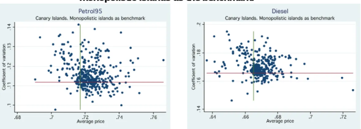
The use of this benchmark enables us to change the perspective of the analysis shown in Figure 1. In Figure 2 the horizontal and vertical lines show the average coefficient of variation and average price of the monopolistic islands respectively, thus reflecting the least competitive market structure. In this case we are looking for gas stations that have coefficients of variation similar to those of perfect collusion (monopoly). As we can see, the concentration of points for both products is close to the average coefficient of variation for the monopolistic islands.
Figure 2. Price and coefficient of variation for petrol 95 and diesel (all gas stations) using the monopolistic islands as the benchmark.
Source: own elaboration compiled from data provided by the Ministry of Industry, Tourism and Trade. Note: average prices are expressed in euros per liter of fuel.
Taking as our reference the behavior of the monopolistic islands, we can draw one important conclusion: gas stations in an oligopoly have a higher coefficient of variation. This means that we obtain evidence of a positive relationship between monopolistic behavior and price rigidity.
The main advantage of this case is the existence of a real monopoly in two of the seven geographic markets analyzed, which in the literature (as far as we know) has never before been the case. In fact comparing monopolistic islands with oligopolistic markets is an ideal situation. All gas stations on the monopolistic islands show the same prices on both islands, but they are not the highest in all the markets. This reflects the vast difference in demand between these markets that we mentioned earlier. In fact Perdiguero and Jiménez (2009) examined the same market using a conjectural variation analysis emphasizing that the population was a statistically significant factor affecting the quantity sold and, indirectly, the price12.
We can, however, draw a significant conclusion: the coefficient of variation of the companies on oligopolistic islands is always on average above those of the monopolistic islands. The percentage change in the coefficient of variation for each island with respect to that of the monopolistic islands is between 1.06% and 8% higher in the oligopolistic islands (t-test accept differences in mean between two groups, at 13-16% of probability, for petrol 95 and diesel respectively). In summary, monopolistic firms yield a more rigid price behavior than their oligopolistic counterparts.
12
A further explanation is the lower transport costs incurred by the monopolistic islands due to their greater proximity to the refinery in Tenerife. However, the little weight attributed to transport in total costs makes this unlikely. The possibility that there were significant differences in the demand elasticities does not seem to be the explanation. It is hard to imagine greater demand elasticity in monopoly than in oligopoly.
ii) If a very competitive company exists
The question remains as to how best to analyze the situation if there is no monopoly to serve as a benchmark. One option is to identify companies that are known to be more competitive than the rest. This approach was adopted by Brannon (2003) and Esposito and Ferrero (2006) for their respective cases. In the retail gasoline market, Hastings (2004) and Clemenz and Gugler (2004) suggest that only independent firms increased competition in this market.
As mentioned earlier, in the Canary Islands there are no gas stations run by supermarkets (which traditionally compete more aggressively as regards pricing), but there is a company that operates in a similar way and which sells more cheaply, namely PCAN. As we mentioned in footnote 11, PCAN has both a lower value brand and fewer vertical restrictions with wholesalers than branded gas stations.
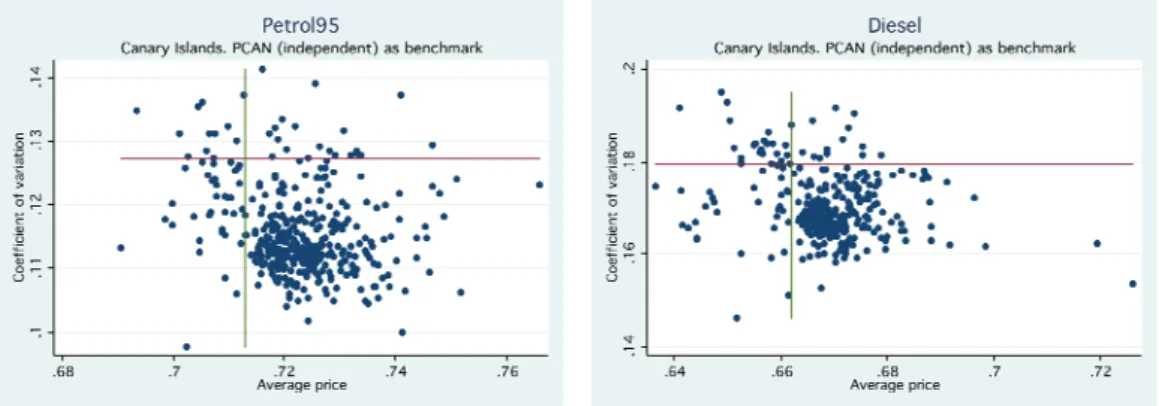
Figure 3 uses the average price and coefficient of variation for PCAN gas stations in the Canary Islands as a benchmark. The objective is to find whether there are retailers in quadrant IV with higher prices and lower coefficients of variation. As can be seen, the vast majority of stations are located in this quadrant.
Figure 3. Price and coefficient of variation for petrol 95 and diesel (all gas stations) using PCAN (independent) as the benchmark.
Source: own elaboration compiled from data provided by the Ministry of Industry, Tourism and Trade. Note: average prices are expressed in euros per liter of fuel.
Likewise, most gas stations have higher prices and lower coefficients of variation when compared with the average figures recorded at PCAN’s pumps. Table 5 shows the average price and coefficient of variation percentages for each brand with respect to PCAN.13
Table 5: Percentage variation in average prices and coefficients of variation for each brand with respect to PCAN (independent brand)
Petrol 95 Diesel
Brand Price (euros) Coefficient of
variation Price (euros)
Coefficient of variation Cepsa 1.1 -9.80 0.9 -5.89 Disa 1.1 -13.06 1.5 -5.63 Shell 1.3 -11.01 1.1 -7.70 British Petroleum (BP) 1.7 -11.38 1.1 -6.04 Repsol 1.1 -7.63 0.3 -5.33 Texaco 1.8 -10.42 1.4 -4.66 Others 1.5 -8.01 1.2 -4.52 Total 1.3 -9.93 0.9 -5.89
Source: own elaboration.
The average prices of other brands are between 0.3% and 1.8% higher than PCAN's, while PCAN's average coefficient of variation is always between 4.5% and 13.1% greater than that of its competitors. A possible explanation for this price pattern could be the location of the gas stations belonging to each brand. However, as shown in Table 6, the distribution of pumps is very similar for all brands.14
In fact PCAN, in common with the other brands, shows a preference for urban locations (see Table 6) and actually has more gas stations in towns than its competitors. For example, five PCAN gas stations (19% of its total) operate as a monopoly in their towns. Despite this advantage of being able to set higher prices, they remain the cheapest of all brands.
13
A t-test analysis shows that the average prices and coefficients of variation between PCAN gas stations and others are different.
14
As seen in Perdiguero and Jiménez (2009), neither are there any significant differences in the number of complementary services (shops, restaurants, etc.) offered by the brands.
Table 6: Brands by population (percentage)
Type of town Repsol Disa (*) Texaco BP PCAN Population < 2,000 3.7 1.8 0.0 0.0 7.7 2,000<Pop<5,000 3.7 4.5 2.9 0.0 0.0 5,000<Pop<10,000 11.1 10.7 14.7 10.7 15.4 10,000<Pop<20,000 33.3 14.3 17.6 10.7 11.5 20,000<Pop<30,000 0.0 13.4 11.8 10.7 19.2 Pop > 30,000 48.1 55.4 52.9 67.9 46.2 Source: own elaboration. (*) Disa is also CEPSA and Shell.
In order to test whether PCAN stimulates competition, we adopted two empirical approaches. The first involved obtaining two values (those of prices and the coefficient of variation) for towns with and without PCAN gas stations. The results suggest that prices are always higher and the coefficient of variation smaller if PCAN is not present. Specifically, prices in towns with PCAN gas stations were 0.4% lower for petrol 95 and 0.3% lower for diesel, while the coefficients of variation were 2.2% and 0.6% higher respectively. In the case of petrol 95, both differences are statistically significant at 1%, while for diesel they are 5% for the price and 10% for the coefficient of variation.
In the second approach we measured the influence of PCAN on the behavior of the other brands by estimating different models.
The first approximation is a logit model. In this estimation the dependent variable takes a value of 1 if the gas station is in the fourth quadrant (higher prices and lower coefficient of variation)15
15
compared to the number of PCAN rivals within a half-mile radius16, the number of rivals from other brands and the number of its own brand pumps.17
We also included a set of control variables: first, a dummy variable that takes a value of one if the observation belongs to diesel fuel and a value of zero in the case of petrol 95; second, the percentage of rivals that are in the fourth quadrant; third, a set of binary variables that reflected the effect of different brands; fourth, a set of binary variables that reflected whether the gas station offered a range of services (including shop, cafe, restaurant, 24-hour opening, car wash and garage services); and finally we calculated the distance from each gas station to the only motorway in Tenerife18.
In the second approximation we construct a left hand side (LHS) variable that is the weighted average of average prices and coefficients of variation. This is expressed as:
0
( )
Averageprice
i
(1
)
CV
i
jX
ji
i 0( )
Averageprice
i
jX
ji
(1
)
CV
i
i 0 j(1
)
i i jiAverageprice
X
CV
i
where “AveragePrice” is the average price and “CV” is the coefficient of variation of every gas station. “Xji” includes the same control variables as in the logit estimation. Using a nonlinear
estimator we can estimate parameters
0,
j, and .
The third approximation is similar to the previous one, but the LHS variables are the weighted average of distance of each average price and the coefficient of variation from the overall means
16
We believe that the “number of PCAN rivals within a half-mile radius” variable may be endogenous. Therefore we apply a two-stage approach. First we regress the number of PCAN rivals against the following variables: a binary variable with the characteristics of the nearest rival, a binary variable with the brand of the nearest rival, and a binary variable of the town and the population of the town where the gas station is
located. However, the R2 of the first stage is very low, so the weakness of the instruments does not correct
the endogeneity problem. It must bestressed that if the PCAN gas stations are located in places where the
price was higher, the coefficient would be biased toward a minor value, so the real effect would be even greater.
17
To perform this analysis we first georeferenced all gas stations operating on the seven islands and then calculated the minimum Euclidean distance between each. The Matlab codes used in these calculations are available from the authors on request.
18
Table 7 shows that the number of observations is smaller than that for the whole sample. There are five explanations for this: 1) the islands of El Hierro, La Gomera and Gran Canaria have no PCAN gas stations and so were excluded from the sample; 2) not all the gas stations on the other islands were georeferenced as no correct coordinates were available; 3) not all the georeferenced gas stations provided information about their services; and 4) there is only one motorway (on the island of Tenerife), therefore the analysis that takes into account the distance to this highway only considers the gas stations on this island, 5) We exclude PCAN gas stations as they would be 0 in the variable "number of PCAN rivals”.
of the two variables, and the angle degree formed for each point to the spot formed by the overall means of the two variables. This expression is:
0
( )
AngleDegree
i
(1
)
Dist
i
jX
ji
i i 0(1
)
Dist
i
jX
ji
AngleDegree
i
0 (1 ) (1 ) (1 ) (1 ) j i i ji i Dist
X
AngleDegree
where “Disti” is the diagonal distance of each average price and coefficient of variation for each
gas station i from the overall means of these two variables for the gas stations located in all four quadrants. In the first quadrant, the greater the distance the more competitive the behavior of the gas stations. However, this relationship is the opposite for those gas stations located in the fourth quadrant: the greater the distance the less competitive the behavior.
To solve this problem we convert the distance in the fourth quadrant into negative values in such a way that the value of the variable distance is smaller as we move away from the mean. Because the interpretation of distance from the average and competitive behavior for the gas stations located in the second and third quadrants is hard,19 we remove these observations from our database . 20
The construction of the "AngleDegree" variable was complex too. Because gas stations are more competitive in the first quadrant, we set the diagonal of the first quadrant as angle zero. Therefore the diagonal of the fourth quadrant, the less competitive gas stations, remains at an angle of 180 degrees. This means that as the angle decreases from 180 to 0 degrees, the behavior of the pump is more competitive (lower prices and higher coefficients of variation).
However, the relationship above 180 degrees is the opposite. As the angle increases from 180 to 360 degrees, this means that the behavior of the gas station is more competitive. To solve this problem we calculate the angle complementary to the gas stations located between 180 and 360 degrees. Thus as the behavior of the gas stations becomes more competitive, the angle assigned to the pump is smaller.21
19
In the second quadrant a higher distance means a higher price but a higher coefficient of variation too, and in the third quadrant it means a lower price but also a lower coefficient of variation.
20
If instead of eliminating the observations we impose a value equal to 0 for the gas stations located in the third and fourth quadrants, the conclusions do not change significantly.
21
We made another specification “in the spirit of” Tobit analysis, where the endogenous variable is a weighted average between these two variables for the gas stations located in the fourth quadrant and 0 for the rest. The results are not provided here because they do not change significantly.
As in the previous approximation, by using a nonlinear estimator we can estimate parameters
0
,
jand .
Finally we apply a multinomial logit, where the endogenous variable takes the value of the quadrant where the gas station is located.
The econometric results of the first three approximations can be seen in Table 7 and the result of the multinomial logit can be seen in Table 8 22 . 23
22
In order to de-trend the data and as a robustness check, we have applied a new coefficient of variation by using standard errors from OLS regressions of prices against a time trend for each gas station. Then we repeat this using graphs and estimations and conclude that the results are not appreciably different.
23
A Chow test has been implemented to test whether petrol 95 and diesel have to be estimated pooled or separately. In all cases the Chow test shows that at 10% we cannot reject the null hypothesis that the coefficients of petrol 95 and diesel are the same. Therefore the estimation can be made by pooling.
Table 7: Econometric results
First approximation Second approximation Third approximation Constant 0.015 (0.189) 0.354 (0.234) 0.194 (0.333) 0.864*** (0.099) 0.821*** (0.094) 0.779*** (0.088) 0.014*** (0.001) 0.013*** (0.002) 0.013*** (0.002) No. rivals PCAN -0.579* (0.307) -0.746** (0.326) -0.598* (0.358) -0.006*** (0.001) -0.006*** (0.001) -0.005*** (0.001) 0.005*** (0.002) 0.005*** (0.002) 0.004*** (0.001)
No. rivals not PCAN 0.143 (0.157) 0.097 (0.160) -0.051 (0.191) -0.002*** (0.001) -0.002*** (0.001) -0.00002 (0.001) 0.001 (0.001) 0.001 (0.001) 0.00004 (0.0006) No. own brand -0.352
(0.221) -0.219 (0.227) 0.151 (0.340) 0.001 (0.001) 0.002** (0.001) 0.001 (0.001) -0.001 (0.001) -0.001 (0.001) -0.002 (0.001) Diesel 0.166 (0.209) 0.149 (0.217) 0.442 (0.270) -0.053*** (0.001) -0.054*** (0.001) -0.053*** (0.001) 0.0004 (0.001) 0.001 (0.001) 0.002** (0.001) % 4th quadrant 0.002 (0.004) 0.0004 (0.004) 0.011 (0.008) 0.00006*** (0.00002) 0.00005*** (0.00002) 4.82e-06 (0.0002) 0.00003 (0.00003) 0.00003 (0.00003) 0.00002 (0.00002) BP -0.045 (0.321) -0.019 (0.343) -0.309 (0.439) 0.003** (0.001) 0.004** (0.002) 0.006*** (0.002) -0.001 (0.001) 0.0001 (0.002) -0.001 (0.002) Repsol -0.848** (0.339) -0.525 (0.426) -0.117 (0.577) -0.002 (0.002) -0.001 (0.002) -0.002 (0.002) -0.0037 (0.0024) -0.004 (0.004) 0.001 (0.003) Texaco -0.050 (0.294) 0.084 (0.321) -0.401 (0.371) 0.003** (0.002) 0.003** (0.002) 0.004*** (0.001) -0.0035* (0.0018) -0.004* (0.002) -0.002 (0.001) Shop -0.345 (0.251) -0.145 (0.346) -0.001 (0.001) -0.0004 (0.001) 0.0001 (0.002) -0.001 (0.002) Cafe 0.088 (0.361) -0.547 (0.433) -0.003* (0.002) -0.002 (0.001) 0.001 (0.002) -0.002 (0.002) Restaurant -0.165 (0.515) -0.104 (0.555) -0.005* (0.003) -0.005** (0.002) -0.003* (0.002) -0.003 (0.002) 24 hours 0.049 (0.304) 0.020 (0.374) -0.003** (0.001) -0.0004 (0.001) 0.001 (0.002) 0.001 (0.002) Car wash -0.079 (0.284) 0.045 (0.378) 0.001 (0.001) -0.0001 (0.001) 0.00002 (0.002) 0.001 (0.002) Garage -1.167*** (0.424) -1.110* (0.591) 0.002 (0.002) -0.0003 (0.002) 0.001 (0.004) 0.002 (0.004) Distance to highway 0.126* (0.065) 0.0001 (0.0001) -1.72e-07 (1.02e-07)
1.169*** (0.118) 1.116*** (0.094) 1.072*** (0.106) -0.0002*** (8.53e-06) -0.0002*** (9.17e-06) -0.0002*** (0.00001) No. Obs. 392 377 260 392 377 260 232 222 158 Wald Chi2 19.41** (0.0128) 27.96** (0.0144) 27.64** (0.0239) (Pseudo for first approximation) R2 0.0370 0.0603 0.0904 0.8954 0.9023 0.9456 0.6107 0.6063 0.6574Table 8: Econometric results of multinomial logit. F.Q. S.Q. T.Q. F.Q. S.Q. T.Q. F.Q. S.Q. T.Q. Constant -0.729*** (0.261) -0.632*** (0.239) -1.074*** (0.281) -1.026*** (0.347) -0.320 (0.281) -1.472*** (0.374) -0.537 (0.463) -0.377 (0.369) -1.805*** (0.548) No. rivals PCAN 1.280*** (0.387) 0.203 (0.441) 0.693 (0.443) 1.614*** (0.430) 0.271 (0.463) 0.927** (0.446) 1.266** (0.544) 0.222 (0.523) 1.377*** (0.521) No. rivals not PCAN -0.408* (0.235) 0.049 (0.192) -0.280 (0.270) -0.389 (0.250) 0.109 (0.203) -0.138 (0.274) -0.210 (0.268) 0.137 (0.228) 0.271 (0.321) No. own brand 0.278 (0.279) -0.592* (0.321) 0.717** (0.292) -0.010 (0.305) -0.444 (0.358) 0.687** (0.315) -1.000* (0.609) -0.336 (0.433) -0.541 (0.447) Diesel -0.224 (0.314) 0.216 (0.265) 0.082 (0.304) -0.181 (0.325) 0.276 (0.276) 0.156 (0.317) -0.226 (0.427) 0.156 (0.319) -0.164 (0.417) % 4th quadrant 0.004 (0.006) 0.002 (0.005) 0.001 (0.006) 0.008 (0.005) 0.001 (0.005) 0.001 (0.007) -0.010 (0.011) -0.501 (0.450) 0.001 (0.012) BP -0.650 (0.501) 0.082 (0.371) -1.588*** (0.602) -0.178 (0.565) 0.147 (0.417) -1.812** (0.699) -0.849 (0.783) -0.055 (0.496) -2.888* (1.616) Repsol -0.284 (0.465) -0.893 (0.591) 0.974*** (0.371) -0.011 (0.626) -1.369** (0.689) 0.634 (0.535) -1.215 (1.013) -0.650 (0.845) 1.550** (0.777) Texaco -1.156** (0.530) -0.176 (0.351) -0.769 (0.471) -1.107** (0.549) -0.218 (0.368) -1.195** (0.516) -0.553 (0.542) -0.273 (0.460) -0.722 (0.643) Shop -0.473 (0.370) -0.490 (0.346) 0.062 (0.375) 0.006 (0.527) -0.501 (0.450) -0.112 (0.537) Cafe 0.222 (0.527) -0.013 (0.465) -0.021 (0.490) 0.300 (0.602) -0.450 (0.517) 0.116 (0.645) Restaurant -0.582 (0.979) 0.358 (0.651) 1.171* (0.653) -0.269 (1.060) 0.689 (0.689) 2.089** (0.861) 24 hours 0.181 (0.429) -0.562 (0.438) -0.048 (0.450) -0.403 (0.553) -0.383 (0.473) -0.110 (0.619) Car wash 0.661 (0.401) -0.288 (0.387) 0.292 (0.414) 0.370 (0.568) -0.096 (0.449) 0.724 (0.608) Garage 0.294 (0.692) 0.656 (0.529) 1.434*** (0.511) 0.280 (0.918) 1.074 (0.688) 0.675 (0.740) Distance to highway -0.310*** (0.111) -0.001 (0.051) -0.004 (0.095) No. Obs. Wald Chi2 Pseudo R2 392 77.61*** (0.0000) 0.0732 377 110.39*** (0.0000) 0.1104 260 83.72*** (0.0004) 0.1195 Note: robust standard error in brackets. *** (1%), ** (5%), * (10%).
It can be seen that the variable number of PCAN rivals located within a half-mile radius is consistently significant. In the first and second approximations the econometric result indicates that the presence of an independent gas station has a negative impact on the likelihood of higher pricing and a more rigid pricing structure, which is consistent with less competitive behavior.
Therefore there would seem to be a correlation between the presence of a PCAN gas station and higher competition (lower prices). In the third approximation the impact of PCAN rivals is positive and significant at 1%. As
is negative in this case, the relationship between PCAN rivals and competitive behavior is the same. A higher number of PCAN rivals increases the distance and reduces the angle degree, so this has a positive impact on the competitive behavior of the gas stations.In the fourth approximation, the multinomial logit model, the econometric results show the same conclusion. The presence of PCAN rivals increases the probability of moving from the fourth to the first quadrant, so the presence of PCAN rivals increases the probability of more competitive prices. It is true that PCAN rivals also increase the probability of passing from the fourth to the third quadrant, but with less intensity.
With these results we can conclude that the presence of an independent retailer within a half-mile radius is correlated to lower and more flexible gasoline prices.
There are a number of issues to discuss regarding the control variables. First, the variable that shows the percentage of competitors in the fourth quadrant is positive and significant in two of the estimations. This result indicates that there might be some geographical "clumping", although it would be mild24. Therefore it is unlikely that there is a formal collusive agreement, but the presence of PCAN in the market significantly increases the level of competition, resulting in lower and more flexible prices.25
Second, the variables that cover the services offered by gas stations and the distance to the highway do not seem to have a significant effect on price behavior.
24
We calculate the percentage of gas stations in a half-mile radius of each point of sale located in the fourth quadrant. The statistical results show that the gas stations located in the fourth quadrant have a higher percentage of gas stations in a half-mile radius also located in the fourth quadrant. Specifically, gas stations located in the fourth quadrant have 19.37% of gas stations in a half-mile radius also in the fourth quadrant, whereas gas stations not located in the fourth quadrant have only 7.78% of gas stations in a half-mile radius located in the fourth quadrant.
25
This result is similar to the entry effects of Wal-Mart on prices. This has been studied in several papers, which conclude that prices decline after its entry. See for example Basker (2005), Basker and Noel (2009) and Lira et al (2007) for the Chilean market.
Summary of results
Analyzing the results of the variance filter without comparing them to a benchmark did not enable us to draw any definitive conclusions. However, applying the two types of benchmark mentioned above yielded the following conclusion: most of the gas stations present behavior that is very close to being monopolistic and are clearly less competitive than the independent company, PCAN.
Although the coefficient of variation for gas stations operating in oligopolies is higher than for their counterparts in a monopolistic situation and lower than PCAN's, the conduct of the gas stations is closer to the former than to the latter. We can therefore conclude that the average performance of the gas stations (excluding those run by PCAN) is very close to that shown on a monopolistic island.
This evidence would certainly justify further investigation of their behavior by the competition authorities. As we have stressed, the variance filter is a suitable technique for detecting possible cartels and for selecting markets for further analysis (i.e. structural analyses that can take into account demand functions, costs, etc.).
This result is not surprising if we take into account the characteristics of the gasoline market in the Canary Islands and the empirical evidence presented above. Moreover, this retail market conforms to most of the factors that facilitate tacit collusion as described by Ivaldi et al. (2003) and the ABA (2010): namely symmetrical costs, transparency of information, etc.
Furthermore, this market also conforms to some of the factors that give rise to price rigidity. For example, Athey et al. (2004) confirm that price rigidity can arise if companies know their rivals’ costs. In this case all companies share the same wholesaler.
Genesove and Mullin (2001) suggest market transparency as a way of controlling price variability, and this gasoline market is certainly highly transparent. Connor (2005) argues that preventing or limiting entry increases the likelihood that price variation will be reduced. Without actually accusing the companies here of forming part of a cartel, entry might be low in this sector either for environmental reasons or because of the difficulty in obtaining licenses to open gas stations in new areas, especially with the current stagnation in demand, even at high fixed (and sunk) costs.
Empirical evidence obtained by adopting other approaches also supports a conclusion of non-competitive behavior. The results obtained by Jiménez and Perdiguero (2008) and Perdiguero
and Jiménez (2009) using conjectural variation analyses show that the typical behavior of gas stations operating in oligopolistic markets is close to perfect collusion. Indeed the authors cannot rule out the possibility that retailers behave as a monopoly.
Thus, while the aggregate analysis carried out here does not allow us to conclude that collusive behavior exists, the application of two benchmarks (a monopoly island and a company with a more aggressive attitude to price competition) together with the results of other structural approaches to this sector allow us to conclude that the retail gasoline market could be more competitive than it currently is, and, while no companies exercise effective competition (such as PCAN), the implicit behavior of the firms is more pro-collusive than pro-competitive.
6. Conclusions
The detection, analysis and prosecution of cartels are the competition authorities’ main tasks. However, detecting cartels is by no means straightforward. Therefore the development of simple methods requiring only a relatively low level of data for identifying possible collusive behavior can be of great use.
The variance filter satisfies these requirements and has therefore become popular in recent years. However, despite its popularity, two aspects have remained undiscussed to date, namely the existence of the relationship between market structure and price rigidity, and the implementation of different types of benchmark for interpreting results.
This article has sought to shed light on these issues by applying a variance filter to the retail gasoline market in the Canary Islands (Spain). The islands are unusual in that the market on five of them is in the form of an oligopoly while that on the remaining two is monopolized by the DISA company. This particular market structure has enabled us to determine whether monopoly prices were more or less rigid in comparison with a potentially more competitive market and thus draw conclusions about the level of competition.
Our empirical results have shown, firstly, how the retailers on monopolistic islands presented lower coefficients of variation than those on other islands, thereby confirming that lower competition in markets tends to lower price variability. Secondly, the comparison of results obtained for the monopoly in gas stations and for the independent company (PCAN) suggests that the situation recorded is closer to perfect collusion than to a competitive outcome. Jiménez and
Perdiguero (2008) and Perdiguero and Jiménez (2009) report similar conclusions, albeit by applying different methodologies.
The appropriateness of such tools as collusive markers should be stressed. The empirical evidence presented here should serve to consolidate methodologies that confirm the existence of more rigid prices in the presence of a cartel and make it easier to interpret results using different benchmarks.
Note, however, that it is important to correctly define the benchmark of comparison when adopting this method so as to ensure a truly practical way for the competition authorities to operate. In this particular instance we have used monopolies, but when this is not possible and there is no known period of collusion, we have seen that the behavior of independent gas stations could serve as a reference.
As the ABA (2010) explains, although in theory it might seem that parallel pricing (and other parallel practices) might merely reflect independent behavior determined by expectations of the way in which competitors will respond, the law has developed to where the burden is on the plaintiff to identify any possible “plus factors”, i.e. additional evidence or indicators of coordinated action.
However, the ABA goes on to state that: “(…) when sellers recognize their interdependence and compete during a number of time periods, their interactions may evolve from non-cooperative oligopoly into tacit collusion without communication of an explicit agreement”. This would appear to be the case in the situation we have described here.
References
Abrantes-Metz, R.M., Pereira, P. (2007). The impact of entry on prices and costs. SSRN-Working paper. [Online]. Available at: http://papers.ssrn.com/sol3/papers.cfm?abstract_id=1013619
Abrantes-Metz, R.M., Bajari, P. (2009). Screens for conspiracies and their multiple applications. Antitrust, Fall 2009.
Abrantes-Metz, R.M., Froeb, L.M., Geweke, J.F., Taylor, C.T. (2006). A variance screen for collusion. International Journal of Industrial Organization, 24, 467-486.
Abrantes-Metz, R.M., Kraten, M., Metz, A., Seow, G. (2008). LIBOR manipulation?
SSRN-Working Paper. [Online]. Available at: http://papers.ssrn.com/sol3/papers.cfm?abstract_id=1201389
American Bar Association (2010) Economic Expert Testimony. In: Proof of Conspiracy under Federal Antitrust Laws, United States, pp. 209-243.
Athey, S., Bagwell, K., Sanchirico, C. (2004). Collusion and price rigidity. Review of Economic Studies, 71, 317-349.
Baker, J.B. (1993). Two Sherman Act Section 1 Dilemmas: Parallel Pricing, the Oligopoly Problem and Contemporary Economic Theory. The Antitrust Bulletin, 38(1), 143-219.
Basker, E. (2005). Selling a cheaper mousetrap: Wal-Mart´s effect on retail prices. Journal of Urban Economics, 58, 203-229.
Basker, E., Noel, M. (2009). The evolving food chain: competitive effects of Wal-Mart´s entry into the supermarket industry. Journal of Economics and Management Strategy, 18(4), 977-1009.
Bolotova, Y., Connor, J.M., Miller, D. (2008). The impact of collusion on price behavior: Empirical results from two recent cases. International Journal of Industrial Organization, Vol. 26(6), 1290-1307.