Nonparametric circular methods for density and regression

(1)

NONPARAMETRIC CIRCULAR METHODS

FOR DENSITY AND REGRESSION

Mar´ıa Oliveira P´erez

Departamento de Estat´ıstica e Investigaci´on Operativa Universidade de Santiago de Compostela

(2)

(3)

Todas as cousas son imposibles, mentres o parecen. Concepci´on Arenal

(4)

(5)

Prof. Dra. Rosa Mar´ıa Crujeiras Casais e Prof. Dr. Alberto Rodr´ıguez Casal, do Depar-tamento de Estat´ıstica e Investigaci´on Operativa da Universidade de Santiago de Compostela, informan que a memoria titulada:

NONPARAMETRIC CIRCULAR METHODS FOR DENSITY AND REGRESSION

foi realizada baixo a súa dirección por Dona Mar´ıa Oliveira Pérez, estimando que a interesada se atopa en condicións de optar ao Grao de Doutor en Estat´ıstica e Investigación Operativa, polo que solicitan que sexa admitida a trámite para a súa lectura e defensa pública na Facultade de Matemáticas da Universidade de Santiago de Compostela.

En Santiago de Compostela, a 11 de setembro de 2013.

Os directores:

Prof. Dra. Rosa Mar´ıa Crujeiras Casais

Prof. Dr. Alberto Rodr´ıguez Casal

(6)

(7)

Introduction

This essay is focused on the analysis of circular data. Circular data are a particular case of directional data where observations are directions in two dimensions. As its name suggests, circular data can be represented as points on the circumference of a unit circle centered at the origin and are usually expressed as angles. Hence, in order to define a circular observation, an initial direction and a sense of rotation must be chosen. The data analysis cannot depend on these ad hoc choices. Moreover, circular data have a periodic structure. All these features make them different from the usual linear data and so, it seems obvious that such data cannot be treated in the same way. Some general references on circular statistics, or more general directional data analysis, are Mardia (1972), Batschelet (1981), Fisher (1993), Mardia and Jupp (2000) and Jammalamadaka and SenGupta(2001).

In recent years, there has been an increasing interest in directional statistics since this kind of data appears in a large variety of disciplines such as biology (in the study of orientation of animals), meteorology (when analyzing wind direction) or environmental sciences (in the study of directions of ocean currents), among others. Two of the most fundamental problems in statistics are knowing how a circular random variable is distributed (density estimation) and how it is related with other variable (regression estimation). In our case, how can be it used to model the behaviour of a scalar response.

Density and regression estimation can be approached from a parametric or from a nonparamet-ric perspective. The parametnonparamet-ric approach assumes that data are drawn from a known parametnonparamet-ric model and the problem is reduced to estimate its parameters. The nonpametric approach does not rely on such somewhat restrictive assumptions and “let the data speak for themselves”. In most of the applied papers dealing with circular data, it is only considered the use of circular descriptive techniques providing graphical displays of the data and classical parametric inferential tools (see, e.g., Arad´ottir et al., 1997; Mooney et al., 2003; Corcoran et al., 2009). Thus, our interest is focused on the analysis of circular data from a nonparametric perspective. Concretely, the main aim of this dissertation is to propose and analyze nonparametric circular methods for density and regression estimation.

In this context, nonparametric density estimation was approached by Beran(1979),Hall et al. (1987) and Bai et al. (1988) who studied the circular kernel density estimator for the general

(10)

2 Introduction

case of directional data. In the regression setting, nonparametric methods involving circular data have been studied by Di Marzio et al. (2009), Qin et al. (2011a,b) and Di Marzio et al. (2012) who proposed kernel smoothers. Periodic smoothing splines introduced by Cogburn and Davis (1974) provide an alternative to kernel estimators when the predictor is a circular variable and the response is linear.

A critical issue in any nonparametric procedure is the smoothing parameter selection. Al-though, some procedures have been proposed byHall et al. (1987),Taylor (2008) and Di Marzio et al. (2011) for circular kernel density estimation, the main contribution in this setting will be the introduction of a new smoothing parameter selector that performs well in very different and complex distributional scenarios. For regression estimation with a linear response and a circular covariate, cross–validation rules are suggested in order to select the smoothing parameter, both for kernel and smoothing spline estimators.

Another important problem in the use of smoothing methods is whether or not observed fea-tures in the smoothed curve, such as peaks and valleys are really there, as opposed to being artifacts of the natural sampling variability. For linear data, the SiZer method developed by Chaudhuri and Marron (1999) both for density and regression estimation allows for the assess-ment of statistically significant features in a smoothed curve and moreover, it avoids the problem of selecting a smoothing parameter. However, nothing similar exists for circular data. With this goal, a new method namely CircSiZer, conveniently adapted to the circular nature of the variables will be introduced in this dissertation.

The manuscript is organized in the following way:

Chapter 1 is devoted to the introduction of circular data, revising some circular distributions and studying the parameter estimation for the von Mises distribution and for mixtures of these distributions. In this chapter, the datasets that motivate and illustrate the methods proposed along the manustript are described.

Chapter2is focused on nonparametric curve estimation. The estimation of the density function is addressed in the first part where the kernel density estimator for circular data is introduced, revising and proposing different methods for selecting the smoothing parameter and checking their behaviour in a simulation study. The second part of this chapter is focused on nonparametric regression estimation for a circular explanatory variable and a linear response. This problem is approached by using kernel smoothers and periodic smoothing splines, which are compared in a simulation study. In both settings, density and regression, the techniques proposed are illustrated with classical data examples and applied to analyze some real datasets.

In Chapter3, in order to assess the significance of the features observed in the smoothed curves, both for density and regression, a SiZer (Significative Zero crossing of the derivative) technique is developed for circular data, namely CircSiZer. The performance of CircSiZer is illustrated with simulated data and finally, the method is used for analyzing some real datasets.

(11)

Introduction 3

methods for density and regression estimation for circular data studied in the previous chapters is described. The library includes most of the self–programmed code which has been implemented for applying the proposed methods in practice.

Finally, the manuscript includes four appendices. In Appendix A, the circular density models used in the simulation study in Chapter 2 and for illustration throughout the manuscript are defined. Appendices B and C give technical details on kernel regression smoothers and periodic smoothing splines, which complement Chapter2and3. AppendixDdescribes the functions in the

NPCirc library, giving instructions about their usage and arguments and illustrating them with examples.

I would like to thank my advisors, Prof. Rosa M. Crujeiras and Prof. Alberto Rodr´ıguez Casal for their work and support during these years. I also wish to thank Prof. Augusto P´erez–Alberti from the Department of Physical Geography of the University of Santiago de Compostela and Dr. Kenneth A. Mann from the Upstate Medical University (New York) for kindly providing some real datasets that motivate part of the work done in this thesis.

This work has been supported by Project MTM2008–03010 from the Spanish Ministry of Sci-ence and Innovation, and by the IAP network StUDyS (Developing crucial Statistical methods for Understanding major complex Dynamic Systems in natural, biomedical and social sciences), from Belgian Science Policy.

(12)

(13)

Chapter 1

Circular models and data

1.1 Introduction

The analysis of circular data appears in many applied fields, such as biology (Batschelet,1981), ecology (Jammalamadaka and Lund,2006), meteorology (Bowers et al.,2000), sociology (Bruns-don and Corcoran, 2005), medicine (Mooney et al., 2003) or biomechanics (Mann et al., 2003), among others.

A circular observation can be defined as a point on a circle of unit radius, or a unit vector in two dimensions (i.e., a direction in the plane). Hence, once an initial direction and orientation of the circle have been chosen, each circular observation can be specified by the angle from the initial direction to the point on the circle corresponding to the observation. More generally, a unit vector in a d–dimensional space (d_≥2) is called a directional data or a spherical data.

Directional data in general, and circular data in particular, have special features both in terms of models and in terms of their statistical treatment. For instance, the numeric representation of a circular obsevation, as an angle or a unit vector, is not necessarily unique since it depends of the initial direction and the sense of rotation. Because of this, another feature of circular data is that there is not a natural ordering of the observations. Moreover, circular data are periodic, i.e., ifθ is an angle in the interval [0,2π) thenθ can be also represented by (θ+ 2πk) for any integer

k. Thus, the methods for dealing with circular data must take into account these features and so, standard real–line methods are not appropriate for analyzing this kind of data.

Circular data analysis has been approached from parametric and nonparametric perspectives, existing a broad literature on parametric methods, both for density and regression. Comprehensive reviews such as Mardia (1972), Fisher (1993), Mardia and Jupp (2000), Jammalamadaka and SenGupta (2001) and Lee (2010) present parametric density models such as the von Mises, the cardiod, or the wrapped distributions, among others, testing procedures for assessing uniformity, such as Rayleigh’s, Kuiper’s, Rao’s Spacing or Watson’s tests, jointly with different correlation coefficients and parametric regression models for two circular variables or a circular and a linear

(14)

6 Chapter 1. Circular models and data

variable.

Some background on circular parametric models and some real data examples are presented in this chapter. Section 1.2 is devoted to the introduction the concept of circular distribution and give a brief overview on the most important circular parametric distribution families, such as the classical von Mises distribution, the cardioid distribution, some wrapped distributions and mixtures of circular distributions. Parameter estimation will be studied for the von Mises distribution and mixture of them. For mixtures, the associated Expectation Maximization (EM) algorithm for carrying out maximum likelihood estimation will be detailed. Finally, in Section1.3, some real datasets that motivate this dissertation will be described. Moreover, these datasets will be considered along the manuscript for illustration purposes.

1.2 Circular parametric distributions

A circular distribution is a probability measure supported on the unit circle. Each point in the circumference represents a direction and so, a circular distribution assigns probabilities to different directions. As for linear data, the distribution of a circular variable can be absolutely continuous. In this case, one way of specifying a distribution on the unit circle is by means of its density function. From now on, any circular random variable Θ will be measured in radians and its support will be the interval [0,2π). Hence, the probability density function is a functionf defined for each angle θ_∈[0,2π) satisfying the conditions:

(i) f(θ)_≥0, θ_∈[0,2π); (ii) R₀2πf(θ)dθ= 1;

(iii) f(θ) =f(θ+ 2πk),_∀θ_∈[0,2π) and any integer k, i.e., f is periodic with period 2π; (see Jammalamadaka and SenGupta,2001, Section 2.1).

Any such function describes a probability distribution on the circle. Let θ1 and θ2 be fixed

angles with 0_≤θ1 ≤θ≤θ2≤2π, then

P[θ1≤Θ≤θ2] =

Z θ2

θ1

f(θ)dθ.

As for linear variables, the characteristic function determines the distribution. The value of the characteristic functionϕ(t) =_E(eitΘ_{) at an integer}_r_{is also called the}_r_{–th trigonometric moment}

of Θ which is given by:

E(eirΘ) = Z 2π 0 eirθf(θ)dθ= Z 2π 0 cos(rθ)f(θ)dθ+i Z 2π 0 sin(rθ)f(θ)dθ, r= 0,_±1,_±2, . . .

where i denotes the imaginary unit. Concretely, the first trigonometric moment, expressed in polar coordinates, is:

(15)

1.2. Circular parametric distributions 7

whereρ is the mean resultant length and µis the mean direction.

The most simple absolutely continuous distribution on the circle is the circular uniform dis-tribution which assigns the same probability to all the directions. When a disdis-tribution is not uniform, this may be concentrated around one or more directions. In that case, the distribution is said unimodal or multimodal, respectively.

An appropriate measure of the mean direction for a set of directions which are unimodal is obtained by treating the data as unit vectors and computing the direction of their average resultant vector. Letθ1, . . . , θn be a set of circular observations given in terms of angles. The sample mean direction ¯θ is then given by

¯ θ= arg    1 n n X j=1 cosθj+i1 n n X j=1 sinθj   .

where arg denotes the function which returns the argument of a complex number. More explicitly, using the notationC =Pn_j₌₁cosθj and S=Pnj=1sinθj, the sample mean direction is given by

¯ θ= arctan∗ S C =                arctan(S/C) if C >0, S _≥0 π/2 if C= 0, S >0 arctan(S/C) +π if C <0 arctan(S/C) + 2π if C_≥0, S <0 undefined if C= 0, S = 0 (1.1)

where the inverse tangent function arctan takes values in [₋π/2, π/2] and so, arctan∗ takes values in [0,2π).

Moreover, the length of the average resultant vector, denoted by ¯R, provides a measure of concentration of the data. If all angles are identical, then ¯R= 1 and if data are widely dispersed then ¯R will be almost 0.

Circular uniform distribution This distribution has a constant density

f(θ) = 1

2π, 0≤θ <2π,

i.e., all directions are equally likely.

Some unimodal distributions are the cardioid, von Mises and some wrapped distributions such as the wrapped normal, the wrapped Cauchy and the wrapped skew–normal distribution. These models are characterized by at least two parameters, one defining the location or reference direc-tion and other defining the dispersion about that locadirec-tion.

(16)

Cardioid distribution

This distribution was introduced by (Jeffreys,1961, p. 328). The cardioid distribution,C(µ, ρ) is a perturbation of the uniform density by a cosine funtion whose density function is:

f(θ;µ, ρ) = 1

2π(1 + 2ρcos(θ−µ)), 0≤θ <2π,|ρ| ≤

1 2.

The mean resultant length of C(µ, ρ) is ρ and (if ρ > 0) the mean direction is µ. When ρ = 0, the cardioid distribution reduces to the circular uniform distribution. This is a symmetric and unimodal distribution around µ.

von Mises distribution

The von Mises distribution is also known as circular normal distribution since it was derived in a way analogous to the derivation of the normal distribution in the real line. von Mises (1918) asked about the existence of a circular model verifying that: for any sample of circular data, the maximum likelihood estimator of the location parameter is equal to the sample mean. Hence, the von Mises distribution was obtained.

The von Mises distribution with parametersµ and κ,vM(µ, κ), is a symmetric and unimodal distribution with density

f(θ;µ, κ) = 1 2πI0(κ)

eκcos(θ−µ), 0_≤θ <2π, (1.2) whereI0 denotes the modified Bessel function of the first kind and order zero which is defined as

follows I0(κ) = 1 2π Z 2π 0 eκcosθdθ.

Here, I0(κ) is a normalizing constant. The parameterµ (0≤µ <2π) is the mean direction and

where the mode is located. The parameter κ (κ _≥ 0) is known as the concentration parameter since the ratio of the density at the mode µ to the density at the antimode (µ+π), where the minimum density is reached, is given bye2κ _{and so, as}_κ _{increases the distribution becomes more} concentrated aroundµ. Whenκ= 0, the distribution reduces to the circular uniform distribution.

Wrapped distributions

Circular distributions can be obtained by wrapping linear distributions onto the circle of unit radius. IfX is a random variable on the real line, this variable may be transformed to a circular random variable Θ by reducing its modulo 2π, i.e.,

Θ =X(mod 2π).

Hence, ifX has density function g, the density function of Θ is given by

f(θ) =

∞

X k=−∞

(17)

(see Jammalamadaka and SenGupta,2001, p. 31).

The wrapped normal and wrapped Cauchy distributions, described below, are some examples of the distributions that can be obtained in this way.

Wrapped normal distribution

The wrapped normal distribution,W N(µ, ρ), is obtained by wrapping the N(µ, σ2) distribution onto the circle, whereρ=e−σ2/2. Its probability density function is given by

f(θ;µ, ρ) = 1 2π 1 + 2 ∞ X k=1 ρk2cosp(θ₋µ) ! , 0_≤θ <2π,

where µ (0 _≤ µ < 2π) is the mean direction and ρ is the mean resultant length. Note that, when ρ goes to zero the distribution becomes less concentrated aroud the mean direction. This distribution is unimodal and symmetric about its mode µ.

Wrapped Cauchy distribution

The wrapped Cauchy distribution, W C(µ, ρ), is obtained by wrapping the Cauchy distribution on the real line with density

g(x;µ, σ2) = 1

π

σ

σ2_{+ (}_x₋_µ₎2, −∞< x <∞

onto the circle. Its density function has the following expression

f(θ;µ, ρ) = 1 2π

1₋ρ2

1 +ρ2₋₂_ρ_cos(_θ₋_µ₎, 0≤θ <2π,

where 0 _≤ µ < 2π is the mean direction and ρ = e−σ is the mean resultant length. It is also a unimodal and symmetric distribution around its modeµ.

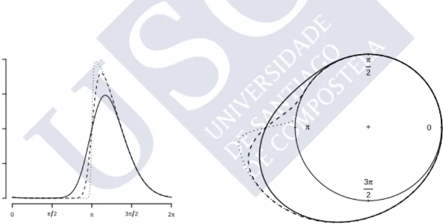
Figure1.1shows the von Mises, cardioid, wrapped normal and wrapped Cauchy densities with the same values for the parameters µ and ρ. Among them, the wrapped Cauchy distribution is noted by its peaked mode.

However, not all circular distributions are unimodal and symmetric. Pewsey (2000) defined a unimodal and asymmetric distribution, namely the wrapped skew–normal distribution.

Wrapped skew–normal distribution

The wrapped skew–normal distribution is a skewed distribution characterized by a location pa-rameter µ (0_≤µ < 2π), a scale parameter κ (κ > 0) and a skewness parameter λ (λ_≥ 0). Its density function is given by

f(θ;µ, κ, λ) = 2 κ ∞ X r=−∞ φ θ₋2πr₋µ κ Φ λ θ+ 2πr₋µ κ ,

(18)

whereφand Φ denote the standard normal density and distribution functions, respectively. This distribution will be denoted byW SN(µ, κ, λ). The asymmetric shape of this distribution can be seen in Figure1.2, for different values of λ.

0 π2 π 3π2 2π 0.0 0.1 0.2 0.3 0.4 0.5 0 π 2 π 3π 2 +

Figure 1.1: Left panel: linear representation of the density functions ofvM(µ, A−1(ρ)) whereA−1

denotes the inverse of function A(_·) = I1(·)/I0(·) (solid line), C(µ, ρ) (dashed line), W N(µ, ρ)

(dotted line) and W C(µ, ρ) (dotted–dashed line) withµ=π and ρ= 0.45. Right panel: circular representation of vM(µ, A−1(ρ)) (solid line) and W C(µ, ρ) (dotted–dashed line).

0 π2 π 3π2 2π 0.0 0.2 0.4 0.6 0.8 0 π 2 π 3π 2 +

Figure 1.2: Linear (left panel) and circular (right panel) representations of a wrapped skew–normal distributionW SN(π,1, λ) withλ= 2 (solid line), λ= 5 (dashed line) and λ= 20 (dotted line).

Further details on these and other distribution models can be found in Fisher (1993), Jam-malamadaka and SenGupta(2001), Mardia and Jupp(2000) and Pewsey(2000).

Although being widely used, the von Mises model and the other models presented may not be flexible enough to capture the underlying structure of multimodal, highly peaked or skewed distributions. Some new parametric models for handling these features have been presented by Abe and Pewsey (2011), who introduced circular models with two diametrically opposed modes, or Jones and Pewsey (2012), who proposed the inverse Batschelet distribution, accounting for skewness and high kurtosis (far from the nicely bell–shaped von Mises distributions). A more flexible model involving mixtures of von Mises distributions was used by Mooney et al. (2003).

(19)

The consideration of mixtures of parametric models may offer a route to capture complex struc-tures, allowing multimodality and/or asymmetry.

Mixtures

A finite mixture ofM circular distributionsfm,m= 1, . . . , M, has density:

f(θ) = M X m=1

pmfm(θ), 0≤θ <2π,

where pm are positive quantities that sum one (pm > 0 and PmM=1pm = 1) and the fm(θ) are circular densities. The quantitiesp1, . . . , pm are known as weights or mixing proportions and the

fm(θ) are called the component densities of the mixture.

A particular case is the mixture of M von Mises distributions whose density is:

f(θ;µµµ, κκκ, ppp) = M X m=1

pmfm(θ;µm, κm), 0≤θ <2π, (1.3)

whereppp= (p1, . . . , pM) withpm >0 andPMm=1pm= 1 are the weights of the component densities,

µµµ= (µ1, . . . , µM)∈[0,2π)M is the vector of circular means andκκκ= (κ1, . . . , κM)∈(R+)M is the vector of concentrations;fm denotes the density function of a von Mises distributionvM(µm, κm), form= 1, . . . , M. 0 π 2 π 3π 2 + 0 π 2 π 3π 2 + 0 π 2 π 3π 2 + 0 π 2 π 3π 2 +

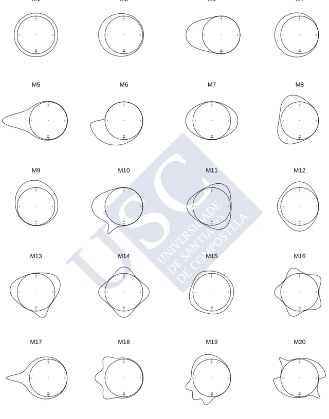
Figure 1.3: Mixtures of von Mises distributions with different number of components. These models correspond to models M7, M9, M11 and M19 defined in AppendixA.

Figure1.3shows four mixtures of von Mises distributions with different number of components, which present multimodality and asymmetry. For example, bimodality arises in the first model setting the mixture proportion to one–half and combining two confronted distributions whereas asymmetry is induced in the second model by considering different weights. The third plot shows a mixture of three von Mises distributions with equally spaced modes and the same concentration parameter. Finally, the last plot is an asymmetric model which is a mixture of five von Mises distributions and only shows four modes. These models will be used in the next chapter and the specific formulae is given in the AppendixA (models M7, M9, M11 and M19).

(20)

1.2.1 Parameter estimation for a von Mises distribution

In this section, the parameters of a von Mises distribution will be estimated by the method of moments and maximum likelihood. Although they are two classical techniques, the estimation procedure in the setting of circular data will be detailed since apart from its usefulness as paramet-ric estimation methods, they will be needed in Chapter 2 for constructing smoothing parameter selectors in a nonparametric setting.

Let Θ1,Θ2, . . . ,Θn∈[0,2π) be a random sample from vM(µ, κ).

Estimation by the method of moments

The modified Bessel function of the first kind and orderr is defined as

Ir(κ) = 1 2π Z 2π 0 cos(rθ)eκcosθdθ, r= 0,1,2, . . . Since 1 2π Z 2π 0 sin(rθ)eκcosθdθ= 0,

the moment of order r of the von Mises probability density is given by 1 2πI0(κ) Z 2π 0 eirθeκcos(θ−µ)dθ = 1 2πI0(κ) Z 2π 0 eir(ω+µ)eκcosωdω = e irµ 2πI0(κ) Z 2π 0

[cos(rω) +isin(rω)]eκcosωdω

= Ir(κ)

I0(κ)

eirµ= Ir(κ)

I0(κ)

[cos(rµ) +isin(rµ)].

The r-th order sample moment is given by 1 n n X j=1 eirΘj ₌ 1 n n X j=1 cos(rΘj) +i1 n n X j=1 sin(rΘj).

By equating population moments with sample moments for r = 1, the equations that define the estimators ˜µ and ˜κ of µand κ by the method of moments are obtained:

A(˜κ) cos ˜µ = 1 n n X j=1 cos Θj, (1.4) A(˜κ) sin ˜µ = 1 n n X j=1 sin Θj, (1.5) whereA(_·) =I1(·)/I0(·).

(21)

If Pn_j₌₁cos Θj 6= 0, by dividing (1.4) by (1.5) results

˜ µ= arctan∗ Pn j=1sin Θj Pn j=1cos Θj ! , (1.6)

where arctan∗is defined in equation (1.1). The method of moments estimator forµis the direction of the sample mean direction.

By multipliying (1.4) by cos ˜µ and (1.5) by sin ˜µ and adding, the equation that defines the method of moments estimator forκ is given by:

A(˜κ) = 1 n n X j=1 cos(Θj−µ˜). (1.7)

So, as long as Pn_j₌₁cos Θj 6= 0, the estimator ofκ, namely ˜κ, is obtained by solving (1.7).

Estimation by maximum likelihood

The maximum likelihood estimators for µ andκ will be those values that maximize the likeli-hood function based on the observations Θ1, . . . ,Θn, i.e.,

L(µ, κ_|Θ1, . . . ,Θn) = n Y j=1 f(Θj;µ, κ) = 1 [2πI0(κ)]n ePnj=1κcos(Θj−µ)_,

or the log–likelihood function

logL(µ, κ_|Θ1, . . . ,Θn) =−nlog(2πI0(κ)) +κ

n X j=1

cos(Θj−µ). (1.8)

From the above expression (1.8), by computing the partial derivatives with respect toµandκ, respectively and equating to zero, the equations that define the maximum likelihood estimators forµand κ, ˆµand ˆκ, are:

ˆ κ n X j=1 sin(Θj−µˆ) = 0, (1.9) A(ˆκ) = 1 n n X j=1 cos(Θj−µˆ). (1.10)

If Pn_j₌₁cos Θj 6= 0, the maximum likelihood estimator forµis obtained from (1.9):

ˆ µ= arctan∗ Pn j=1sin Θj Pn j=1cos Θj !

and ˆκ is obtained from the solution of equation (1.10). Note that, if ˆκ = 0, equation (1.9) is verified and a value for ˆµ can be obtained from the solution of (1.10). However, it can be shown that this solution (ˆµ,ˆκ= 0) is not a maximum of (1.8).

(22)

Thus, the maximum likelihood estimators for the parameters of a von Mises distribution are equal to the ones obtained by the method of moments (see equations (1.6) and (1.7)), i.e., ˜µ= ˆµ

y ˜κ= ˆκ, with probability one.

Figure 1.4 shows the boxplots of the differences in absolute value between the estimated and true values of the parameters of avM(π,1). Parameters are estimated by maximum likelihood by using 1000 random samples of sizen= 100 andn= 500 from that distribution. As it was expected, differences are smaller for the largest sample size. In order to obtain a better visualization, outliers are not plotted in the figure.

µ κ 0.0 0.1 0.2 0.3 0.4 µ κ 0.0 0.1 0.2 0.3 0.4

Figure 1.4: Boxplots of the differences in absolute value between the estimated and true values of the parameters of a von Mises distribution vM(π,1). Results were obtained from 1000 random samples of size n= 100 (left panel) and n= 500 (right panel).

0.0 0.1 0.2 0.3 0.4 0.5 0.6 0 2 4 6 8 10

Figure 1.5: Density function1 of the estimates of the concentration parameter of a von Mises distribution based on 1000 random samples of size n = 100 (dashed line) and n = 500 (solid line) from a mixture of two von Mises distribution (see model M7 in Appendix Afor the specific formulae).

1_{The density functions were obtained by using the kernel density estimator for linear data defined at the beginning}

of Section2.2and taking as smoothing parameter the value selected by the rule of thumb ofSilverman(1986, p. 47).

(23)

In this case, the model is correctly specified and the errors in the parameter estimation are small, so the parametric estimation of the density function should be right. But, what happens when the model is not well specified? For example, consider that the observations come from a mixture of two equally weighted von Mises distribution with diametrically opposed means and the same concentration parameter (such as model M7 defined in Appendix A) but, it is wrongly assumed that the underlying model is a von Mises distribution. When the concentration parameter of a von Mises distribution is estimated based on observations coming from model M7, it is observed that it takes values close to zero as shown in Figure 1.5for 1000 samples of sizen= 100 (dashed line) andn= 500 (solid line). Therefore, if the underlying model is parametrically estimated, assuming a von Mises model, the estimate is close to a circular uniform (concentration parameter close to 0), which is far from the real distribution. Before going into a purely nonparametric approach for density estimation, a parametric method for estimating mixtures of von Mises will be introduced in the next section.

1.2.2 Parameter estimation for a mixture of von Mises distributions

Let Θ1, . . . ,Θn ∈ [0,2π) be a random sample of angles from a mixture of M von Mises distri-butions, as the one presented in (1.3). In order to estimate the parameters of the mixture, the log–likelihood function of the sample is computed

log(L(µµµ, κκκ, ppp_|Θ1, . . . ,Θn)) = log n Y i=1 f(Θi;µµµ, κκκ, ppp) ! = n X i=1 log M X m=1 pmfm(Θi;µm, κm) ! . (1.11) However, the log–likelihood function has a complex expression (it involves the logarithm of a sum) which is difficult to optimize. The main problem lies in the fact that it is not known which density component generates each observation. Assuming that this information is available, i.e., given a vectorZZZ = (Z1, . . . , Zn) such thatZi takes the valuem if Θi was generated by them–th mixture component, then the log–likelihood would be

log(L(µµµ, κκκ, ppp_|Θ1, . . . ,Θn, ZZZ)) = n X

i=1

log (pZifZi(Θi;µZi, κZi)), (1.12)

which has an expression less complicated than (1.11).

For the sake of simplicity, consider the particular case of a mixture of two von Mises, M = 2. In this case, (1.12) becomes

log(L(µµµ, κκκ, ppp_|Θ1, . . . ,Θn, ZZZ)) = X i;Zi=1 log (p1f1(Θi;µ1, κ1))+ X i;Zi=2 log (p2f2(Θi;µ2, κ2)). (1.13)

From (1.13), by computing the partial derivatives with respect toµ1 andκ1 and equating them

to zero, the equations that define the maximum likelihood estimators ˆµ1 and ˆκ1 of µ1 and κ1

respectively, are obtained:

ˆ

κ1

X i;Zi=1

(24)

16 Chapter 1. Circular models and data A(ˆκ1) = 1 n1 X i;Zi=1 cos(Θi−µˆ1) = 0, (1.15)

wheren1 is the cardinality of the set{i: Zi = 1, i= 1, . . . , n}. Note that, if only the data of the first component of the mixture are considered then, these equations are the same to those defined in (1.9) and (1.10). If P_i_;_Z_i₌₁cos Θi6= 0, from (1.14), ˆ µ1= arctan∗ P i;Zi=1sin Θi P i;Zi=1cos Θi ! (1.16)

and ˆκ1 is obtained from the solution of equation (1.15). Maximum likelihood estimators for µ2

and κ2 are obtained in the same way.

Since p1+p2 = 1, equation (1.13) can be written in terms of p, wherep1=p and p2 = 1−p.

Taking the derivative with respect to p and setting it equals to zero, the maximum likelihood estimator ofp is

ˆ

p= ˆp1 =n1/n.

Therefore, the maximum likelihood estimate of the parameters of a mixture of two von Mises distributions is easy to obtain if it is known which density component generates each sample data Θi, i.e., if the values of the variableZZZ are known. However this information is often unknown.

In this latter case, when the sample data is incomplete, the EM algorithm provides a method for estimating the parameters of the mixture by maximum likelihood. The EM algorithm (Dempster et al.,1977) is an iterative proccess which applies two steps alternatively until the convergence:

• E–step: Compute the expected value of the complete data log–likelihood with respect to the conditional distribution of the non observed variable. In our context, the variable that indicates which density component generates each observation is the non observed variable.

• M–step: Estimate the parameters by maximizing the expectation computed in the E–step. Given values forµµµ,κκκ andpppand following this procedure, if p(m_|Θi, µµµ, κκκ, ppp) denotes the condi-tional distribution of the variable Zi, i.e.,

p(m_|Θi, µµµ, κκκ, ppp) =

pmfm(Θi;µm, κm) PM

l=1plfl(Θi;µl, κl)

then, the expectation of (1.12) can be written as: n X i=1 Ep[log(pZifZi(Θi;µZi, κZi))] = n X i=1 M X m=1 log (pmfm(Θi;µm, κm))p(m|Θi, µµµ, κκκ, ppp) = M X m=1 n X i=1 (logpm)p(m|Θi, µµµ, κκκ, ppp) + M X m=1 n X i=1 logfm(Θi;µm, κm)p(m|Θi, µµµ, κκκ, ppp). (1.17)

(25)

The next step, the M–step, consists on the maximization of the expectaction (1.17) with respect to the parameters (µµµ, κκκ, ppp). Banerjee et al. (2005) proved that the mean direction estimator is

ˆ µm = arctan∗ Pn i=1sin Θip(m|Θi, µµµ, κκκ, ppp) Pn i=1cos Θip(m|Θi, µµµ, κκκ, ppp) , m= 1, . . . , M,

which is a weighted version of the estimator in (1.16). The estimator of the concentration param-eter is obtained from the solution of equation

A(ˆκm) = Pn i=1p(m|Θi, µµµ, κκκ, ppp) cos(Θi−µˆm) Pn i=1p(m|Θi, µµµ, κκκ, ppp) , m= 1, . . . , M,

and the estimator ofpm has the following expression

ˆ pm = 1 n n X i=1 p(m_|Θi, µµµ, κκκ, ppp), m= 1, . . . , M.

E–step and M–step are repeated iteratively until the likelihood converges. Each iteration is guaranteed to increase the log–likelihood and the algorithm is guaranteed to converge to a local maximum of the likelihood (Bilmes,1998).

Initialization of the EM algorithm

The EM algorithm needs to be initialized, i.e., it is required initial values of the parameters

µµµ,κκκ and ppp. In order to obtain such starting values, there exist several approaches such as soft– assignment schemes and hard–assignment schemes. Hard–assignments consist in assigning each observation to one component of the mixture in such way that the probability of each observation of belonging to a certain component is 0 or 1. However, in this work, soft–assignments are considered. Let Sim(ω1, ω2) = cos(ω1−ω2), be a measure of similartiy between two anglesω1 and

ω2. The soft–assignments consists in:

1. Take the mean direction of the sample as the global centroid of the data.

2. Starting with this first centroid, if the number of components in the mixture isM then (M₋

1) more centroids are computed. In order to compute them-th centroid (m= 2, . . . , M), the similarity between each point in the sample and each one of the (m₋1) centroids computed before is calculated. For each point in the sample, the maximum value of similarity between that point and each centroid is taken. The m-th centroid will be the sample point with a smaller similarity.

3. Once the M centroids are computed, the dissimilarity (dissimilarty=1-similarity) between each sample point and each centroid is computed.

(26)

• If the sample point is equal to some centroid, i.e., the dissimilarity between the sample point and the centroid is equal to zero then, it is assigned probability one to the corresponding centroid and probability zero to the remaining centroids.

• If the sample point is not equal to any centroid, then the probability of belonging to the group represented by each centroid is representative is computed. That probability is proportional to the inverse of the dissimilarity. Hence, as smaller is the dissimilarity between one sample point and one centroid, larger is the probability of belonging to that group.

This procedure is equivalent to initialize the conditional distributionp(m_|Θi, µµµ, κκκ, ppp),m= 1, . . . , M.

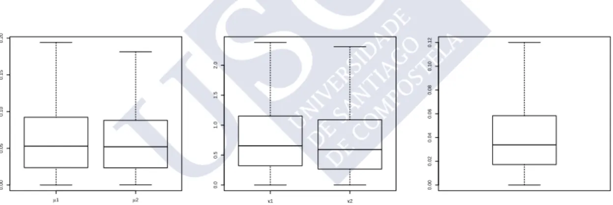
In order to illustrate the performance of the EM algorithm for estimating the parameters of a mixture of von Mises distributions, 1000 random samples of size n= 100 from the first model in Figure 1.3 were generated. Figure 1.6 shows the boxplots of the differences in absolute value between the estimated and true values of the parameters. Figure 1.6 shows that the differences for the mean directions (left panel) and for the proportions (right panel) are small, and they are sligthly larger for the concentration parameters (center panel).

µ1 µ2 0.00 0.05 0.10 0.15 0.20 κ1 κ2 0.0 0.5 1.0 1.5 2.0 0.00 0.02 0.04 0.06 0.08 0.10 0.12

Figure 1.6: Boxplots of the differences in absolute value between the estimated parameters using the EM algorithm and the true values for a mixture of two von Mises distributions, 1/2_·vM(0,4)+ 1/2_·vM(π,4). Results were obtained from 1000 random samples of size n = 100. Left panel: boxplots for the mean directions. Center panel: boxplots for the concentration parameters. Rigth panel: boxplot for the proportion.

Note that in the mixture considered both density components have the same proportion and so, the differences for the mean direction and for the concentration parameters are almost equal for both densities. However, if a mixture of two von Mises distribution in different proportion is considered then, the errors for the component in larger proportion are smaller, as shown in Figure 1.7, where 1000 random samples of size n = 100 from the second mixture in Figure 1.3 have been considered.

(27)

1.2. Circular parametric distributions 19 µ1 µ2 0.0 0.2 0.4 0.6 0.8 1.0 κ1 κ2 0 1 2 3 4 0.00 0.05 0.10 0.15 0.20 0.25 0.30

Figure 1.7: Boxplots of the differences (in absolute value) between the estimated parameters using the EM algorithm and the true values for a mixture of two von Mises distributions, 1/4_·

vM(0,2) + 3/4_·vM(π/√3,2). Results obtained from 1000 random samples of sizen= 100. Left panel: boxplots for the mean directions. Center panel: boxplots for the concentration parameters. Right panel: boxplot for the proportion.

Number of components selection

In order to apply the EM algorithm, the number of components in the mixture must be chosen. If a large number of components (i.e., a larger number of parameters) is considered then overfitting may occur, whereas the opposite effect may occur if that number is small. Determining the number of componentsM can be seen as a model selection problem which can be approached by considering some kind of information criteria, such as the Akaike Information Criterion (AIC). AIC (Akaike, 1974) is a criterion for choosing the best model among a set of admissible models. AIC takes into account the model complexity by means of the number of parameters in the model and the model fit by means of the likelihood function. It has the following expression

AIC =₋2 log(L) + 2d,

wheredis the number of parameters in the model andL is the maximized value of the likelihood function for the estimated model. According to this criterion, one model is better than another if it has a smaller AIC value. So, given a set of models, the best model using the AIC criterion, is one with the lowest AIC.

In the scenarios considered above, it has been assumed that the number of distributions in the mixture is known. However, in most cases, this information is unknown. AIC can be used for selecting the mixture of von Mises distribution that fits the data best. In order to illustrate how this method performs in practice, five models have been considered: the von Mises distribution

vM(π,1) and the four mixtures represented in Figure1.3. The specific formulae of these models can be seen in the Appendix A (models M2, M7, M9, M11 and M19, respectively). For each

(28)

distribution, 1000 samples of size n= 100 andn= 500 were generated and the number of times that the AIC selectsM = 1,2,3,4 and 5 has been computed. Results are shown in Tables1.1and 1.2. For both sample sizes and for the models with three or less components (M2, M7, M9 and M11), it can be seen that AIC selects the right number of components in most cases. However, for the model with more than three components (M19) and sample sizen= 100, AIC tends to select

M = 2 since the number of parameters of the model is too large (14 parameters) in comparison with the sample size. For sample sizen= 500, in most cases AIC selectsM = 4 which corresponds to the number of modes of the model. Note that, in this latter model the AIC criterion does not tend to select the exact number of components (M = 5) because the proportion of one of the components in the model is small and moreover, its concentration parameter is also small and so, this component hardly affects to the model. Therefore, in this particular case, a mixture of four von Mises distribution provides a good approximation.

n= 100 M = 1 M = 2 M = 3 M = 4 M = 5

Model with 1 component (M2) 814 99 53 26 8

Model with 2 components (M7) 0 807 111 60 22

Table 1.1: Number of times that AIC has selectedM = 1,2,3,4 and 5 in a von Mises distribution (M2), mixture of two von Mises (M7 and M9), mixture of three von Mises (M11) and mixture of four von Mises (M19). For each model, results were obtained from 1000 samples of sample size

n= 100.

n= 500 M = 1 M = 2 M = 3 M = 4 M = 5

Model with 1 component (M2) 943 42 11 4 0

Table 1.2: Number of times that AIC has selectedM = 1,2,3,4 and 5 in a von Mises distribution (M2), mixture of two von Mises (M7 and M9), mixture of three von Mises (M11) and mixture of five von Mises (M19). For each model, results were obtained from 1000 samples of sample size

(29)

1.3. Real datasets 21

1.3 Real datasets

In this section, several real datasets will be introduced. Three of them are original datasets which motivated the development of some techniques shown in this dissertation and so, they will be analized as part of this work. The others, corresponding to cross–beds angles and animal orientation data, are classical datasets and they will be used purely for illustrative purposes. A description of all of them is given below:

• Temperature cycle changes.

The International Polar Year addresses as one of the main subjects the quantification and understanding of the environmental change in the polar regions. In particular, monitoring the retreat of glaciers is in the scope of this project. Within this project, measurement sta-tions were placed in periglacial Monte Alvear (Tierra del Fuego, Argentina) (see Figure1.8), recording temperatures hourly at different depths. The ocurrence of changes in cycles of temperature (from frosting to defrosting and viceversa) are important for the analysis of the mobility in the glacier’s surface. The hours when a cycle change has occurred consti-tute a sample of circular data, coming from an unknown circular distribution, that must be estimated in order to determine the cycle change behaviour.

Figure 1.8: Ushuaia region (Tierra del Fuego, Argentina). Monte Alvear and Vinciguerra Glacier.

The available data for studying the cycle change behaviour consist of 350 observations which correspond to the hours when the temperature (measured in ◦C) at ground level changed from positive to negative and viceversa (see Figure 1.9) from February 2008 to December 2009 in periglacial Monte Alvear. This dataset will be analized in Sections2.2.3and 3.6. These data has been kindly provided by Prof. Augusto P´erez Alberti from the Department of Physical Geography of the University of Santiago de Compostela.

(30)

22 Chapter 1. Circular models and data 0h 3h 6h 9h 12h 15h 18h 21h + 0h 3h 6h 9h 12h 15h 18h 21h +

Figure 1.9: Circular plots and rose diagrams of data of hours when the temperature changes from positive to negative (left panel) and viceversa (right panel).

• Wind speed and wind direction.

The Atlantic coast of Galicia (NW Spain) has suffered two major ship accidents which caused serious environmental and ecological damages: the burning of a cargo ship named Cas´on in 1987, and the oil spill of the Prestige tanker in 2002. The strong winds played a decisive role in both accidents. In the first one, the strong winds caused a displacement of the cargo and the corrosive and toxic chemical flamable products trasported by Cas´on exploded and burned while in the Prestige accident, the highly variable and strong winds caused the sinking of the tanker.

N NE E SE S SW W NW 0 5 10 15

Figure 1.10: Left panel: Atlantic coast of Galicia (NW Spain). The plot shows the marine traffic control area (arrows indicate the directions that ships must follow), whithin the influence area of two major lighthouses (white lines). The buoy registering the data is located NE from the traffic control area at longitude -0.210E and latitude 43.500N. Right panel: wind direction is represented over the circumference in clockwise sense, starting form N and wind speed is represented along the radius in m/s.

Motivated by these facts, one question of interest is whether the wind speed may be in-fluenced by the wind direction. A buoy (with a diameter of 1.8 m and a height of 6.5 m)

(31)

anchored in the area at longitude -0.210E and latitude 43.500N (see Figure1.10, left panel) provides hourly collected wind speed and wind direction. Wind measurements regarding direction and speed are recorded every ten minutes, and hourly averaged, at a height of 3 m above sea level. The buoy is far away from the coastline so that the measurements are not influenced by local effects.

Data for studying the relation between wind speed and wind direction consists of hourly observations of wind direction (measured in degrees from North direction) and wind speed (in m/s) in winter season (from November to February) from 2003 until 2012. Data were freely downloaded from the Spanish Portuary Authority (http://www.puertos.es) in July of 2012. Figure1.10(right panel) shows the measurements of wind direction and wind speed. This plot correspond to about 200 observations out of the total data, where observations were taken with a lag period of 95 h for avoiding the dependence present between consecutive measurements in the time series. Since wind direction is a circular variable and wind speed is a scalar variable, the methods for studying the relation between these variables must be take into account the nature of both variables. This data set will be considered in Sections2.3.4 and 3.6.

• Cracks in cemented femoral components.

This real dataset, kindly provided by Dr. Kenneth A. Mann from the Upstate Medical University (New York), concerns angular positions of cracks in the cement mantle in a hip implant. These data, described in more detail in Mann et al.(2003), are obtained from an in vitro fatigue study for investigating the distribution of fatigue cracks around cemented femoral components in total hip replacements.

lateral anterior medial posterior + lateral anterior medial posterior +

Figure 1.11: Rigth panel: a counterclockwise definition of angular position of crack was used with a zero angle representing the lateral direction. Center and right panels: circular plots and rose diagrams of the data of angular positions of cracks for one cemented implant for proximal and distal region, respectively.

Each femur is loaded using a stair climbing apparatus and after loading, it is sectioned in 10 mm intervals from the level of the implant collar to the distal tip of the stem. For

(32)

each section, angular position of the cracks relative to the center of the stem section were documented. A counterclockwise definition of angular position of crack was used with a zero angle representing the lateral direction as shown in Figure1.11 (left panel). In Figure1.11 (center and right panels) the angular positions of cracks for proximal (sections at 10–50 mm) and distal (sections at 80–110 mm) regions are represented. The number of data in each region is 322 and 99, respectively.

Studies to improve understanding of the mechanical aspects of cemented implant loosening were carried out showing that the distribution of the angular positions of the cracks around cemented femoral components is not uniform (see Mann et al., 2003). It is of interest to know if there exists some predominant direction of crack. This will be studied in Section3.6. Apart from the previous datasets, some of which had not been previously studied, and certainly none of them had been analyzed with nonparametric methods, for illustration purposes, some classical datasets will be also considered. Specifically, the following examples will be used in Section2.2.3.

• Cross–beds (I).

This classical dataset corresponds to azimuths of cross–beds in the Kamthi river (India). Originally analized bySenGupta and Rao(1966) and included in Table 1.5 inMardia(1972), the dataset collects 580 azimuths (measured in degrees) of layers lying oblique to principal accumulation surface along the river, being these layers known as cross–beds. A photo of cross–beds is shown in Figure 1.12 (left panel) and data are shown in Figure 1.12 (right panel). 0 π 2 π 3π 2 + 0 π 2 π 3π 2 +

Figure 1.12: Left panel: photo showing cross–beds2_{. Right panel: circular plot and rose diagram}

of data of azimuhts of cross–beds in the Kamthi river.

2_{Rygel, M.C. (2006) Through cross–bedding in the Waddens Cove Formation (Pennsylvanian), Sidney Basin,}

Nova Scotia. File from the Wikimedia Commons.

(33)

• Cross–beds (II).

This dataset, presented inFisher(1993), includes 104 measurements of Chaudwan Zam large bedforms from Himalayan molasse in Pakistan which are represented in Figure 1.13.

0 π 2 π 3π 2 + 0 π 2 π 3π 2 +

Figure 1.13: Circular plot and rose diagram of cross–bed measurements from Himalayan molasse in Pakistan.

• Dragonfly orientation.

Animal orientation is another classical example of circular data. This dataset, presented in Batschelet (1981), contains the orientation of 213 dragonflies with respect to the Sun’s azimuth. As it can be seen in Figure1.14 (right panel), this is a clear example of bimodal circular distribution. This dataset was also studied by Pewsey (2004), who applied a test for circular reflective symmetry.

0 π 2 π 3π 2 + 0 π 2 π 3π 2 +

Figure 1.14: Left panel: image of a dragongly3_{. Right panel: circular plot and rose diagram of}

dragonflies orientations data.

3_{Image of a dragonfly taken with a PackshotCreator photo studio by Creative Tools AB. Date: 27 January}

2010. Source: CreativeTools.se - PackshotCreator - Dragonfly top view. Author: Creative Tools from Halmstad, Sweden. Watermark removed by Ainali.

(34)

(35)

Chapter 2

Nonparametric curve estimation for

circular data

2.1 Introduction

Nonparametric estimation methods have turned up as an alternative approach to the parametric techniques, both inferentially and as a descriptive tool. In the circular setting, nonparametric density estimation was approached byFisher (1989), who proposed an adaptation to circular data of linear data methods in Silverman(1986) using a quartic kernel function andBeran(1979) and Hall et al. (1987), who proposed a kernel density estimation procedure for the general case of spherical data, following the ideas of the classical kernel density estimator for linear data (Parzen, 1962; Rosenblatt, 1956). Although asymptotic properties of this latter estimator were further studied by Bai et al. (1988) and Klemel¨a (2000), these works do not provide a solution for the most critical issue from a practical point of view: smoothing parameter selection. The use of cross– validation smoothing parameters is suggested byHall et al.(1987) in the spherical context, for the particular case of circular data, Taylor (2008) derived a rule of thumb for smoothing parameter selection in circular kernel density estimation and Di Marzio et al.(2011) introduced a bootstrap method for data lying on ad–dimensional torus.

Regression estimation involving circular variables, as response or as covariate, is indeed an interesting problem. In the available literature, most efforts have been focused on the development of parametric models. For instance, Presnell et al.(1998) and the references therein dealt with a circular response and linear covariates;SenGupta and Ugwuowo(2006) proposed some asymmetric models for environmental applications accounting for the circular nature of the covariate, and Downs and Mardia (2002) and Kato et al. (2008), among others, addressed the regression with circular response and covariates. Regression estimation avoiding the assumption of a specific parametric shape for the regression curve was addressed byDi Marzio et al.(2009) who extended least squares local polynomial to the case of d–dimensional circular predictors and real–valued

(36)

28 Chapter 2. Nonparametric curve estimation for circular data

responses;Qin et al.(2011a,b) who extended nonparametric models to the case when there is one circular predictor and one or more linear predictors and the response is real–valued, and more recently Di Marzio et al. (2012) proposed a nonparametric estimator for the regression function when the response is circular and the covariate is circular or linear. Periodic smoothing splines, as considered inWahba(1990) andWood(2006) among others, are an alternative form of smoothing when the covariate is periodic and the response is linear.

The goal of this chapter is to introduce a new procedure for selecting the smoothing parameter in circular kernel density estimation that allows estimating circular densities, accounting for asym-metry and/or multimodality. In the regression setting, a review of the nonparametric methods for a scalar response and a circular covariate will be provided.

This chapter is organized as follows. Section 2.2 is devoted to the introduction of the kernel density estimator for circular data, revising different techniques for selecting the smoothing pa-rameter and introducing a new method. The performance of the described procedures is checked in a simulation study, considering a wide class of circular density families, involving multimodality, peakdness and skewness. The methods are also illustrated with the three classical datasets and the real dataset corresponding to temperature cycle changes. Section 2.3 is devoted to nonpara-metric regression estimation for a circular explanatory variable and a linear response, focusing on the adaptation of the Nadaraya–Watson and Local Linear estimators to the circular nature of the covariate and on periodic smoothing splines. The performance of circular kernel regression estimators and periodic smoothing splines estimator is explored in some simulated examples and they are applied to study the relation between the wind speed and wind direction in the Atlantic coast of Galicia. The contents of this chapter can be seen inOliveira et al. (2012a,b,2013c).

2.2 Nonparametric circular kernel density estimation

Before introducing the circular kernel density estimator, the classical kernel estimator for a density function will be reviewed. Denote byX1, . . . , Xna random sample from a scalar random variable

X with density g. At each fixed point x_∈R, the kernel estimator of g(x) is defined as: ˆ g(x;h) = 1 nh n X i=1 L x₋Xi h , (2.1)

where h > 0 is the bandwidth or smoothing parameter and L is a kernel function, usually the standard normal density, or any other unimodal and symmetric around zero density function. The estimator in (2.1) can be written as follows:

ˆ g(x;h) = 1 n n X i=1 Lh(x−Xi), (2.2)

where Lh is the h–rescaled kernel function L, Lh(·) = _h1L _h·. In the particular case of L being the standard normal, the kernel estimator in (2.2) can be interpreted as a mixture of nnormally distributed random variables, centered in the sample points and with standard deviationh.

(37)

2.2. Nonparametric circular kernel density estimation 29

Since this estimator does not provide a periodic estimate of the density function, its usage is not appropriate for estimating the density function of a sample of circular data. However, bearing the idea of its construction in mind, the kernel estimator in (2.2) can be generalized to circular data.

Given a random sample of angles Θ1, . . . ,Θn∈[0,2π) from some unknown circular density f, the circular kernel density estimator off is defined as:

ˆ f(θ;ν) = 1 n n X i=1 Kν(θ−Θi), 0≤θ <2π, (2.3)

where Kν is a circular kernel function with concentration parameter ν > 0 (see, e.g., Di Marzio et al.,2009). As a circular kernel, the von Mises distribution can be considered. With this specific kernel, the density estimator is given by:

ˆ f(θ;ν) = 1 n(2π)I0(ν) n X i=1 eνcos(θ−Θi)_, ₀_≤_{θ <}₂_π, _(2.4)

which can be seen as a mixture ofnvon Mises distributions, centered in the data sample Θi and with common concentration parameterν. Throughout this dissertation, the circular kernel density estimator with von Mises kernel defined in (2.4) will be considered, unless otherwise indicated.

0 π 2 π 3π 2 + 0 π 2 π 3π 2 +

Figure 2.1: Circular kernel density estimates (gray lines) with ν = 2 (left panel) and ν = 100 (right panel) for 10 random samples of size 200 from a vM(π,5) (black line).

A critical issue when applying this estimator in practice is the choice of the smoothing parameter

ν which determines the degree of smoothing. The effect of the smoothing parameter can be seen in Figure2.1, large values ofνlead to highly variable (undersmoothed) estimators, i.e., estimators with small bias and large variance, whereas small values ofν imply low concentration of the kernel, providing oversmoothed estimators for the circular density, i.e., estimators with large bias and small variance. For that reason the study of automatic smoothing parameter selection procedures constitutes one of the most relevant problems in nonparametric density estimation.

(38)

2.2.1 Smoothing parameter selectors

There are various approaches to the smoothing parameter selection problem. In this section, the methods proposed in the literature will be reviewed and a new method will be introduced.

As for linear data, most commonly used techniques for selecting the smoothing parameter are based on the minimization of some error criteria that quantify the accuracy of the kernel density estimator, i.e., how well the estimator approximates the true density. The mean integrated squared error (MISE), MISE (ν) = _E Z 2π 0 ˆ f(θ;ν)₋f(θ)2dθ = Z 2π 0 E ˆ f(θ;ν)₋f(θ)2 dθ = Z 2π 0 h Efˆ(θ;ν)₋f(θ)i2dθ+ Z 2π 0 E h ˆ f(θ;ν)₋Efˆ(θ;ν)i2dθ = Z 2π 0 h biasfˆ(θ;ν)i2dθ+ Z 2π 0 varfˆ(θ;ν)dθ,

is one of these criteria but, in practice, often its asymptotic expression (AMISE) is used for selecting the smoothing parameter, which may also be written in terms of the aymptotic bias and the variance of the estimator. Precisely, as noted before, a main challenge in nonparametric density estimation is the bias–variance trade–off. Therefore, selecting ν by minimizing either MISE or AMISE amounts to balancing bias and variance at the same time.

In the circular setting, the asymptotic expression for the MISE (AMISE) was derived by Di Marzio et al. (2009). For the circular kernel estimator (2.4), if f′′ is continuous and square– integrable, the AMISE(ν) when ν _{→ ∞}and √νn−1_→_{0 is given by:}

AMISE(ν) = ( 1 16 1₋ I2(ν) I0(ν) 2Z 2π 0 f′′(θ)2dθ+ I0(2ν) 2nπ(I0(ν))2 ) , (2.5)

wheref′′denotes the second–order derivative of the target density to be estimated, which measures the curvature of f. Densities with marked modes will give a larger value of its integral, whereas the lowest value is achieved by a circular uniform model.

Arule of thumb, adapting the idea ofSilverman(1986) for bandwidth selection in kernel linear density estimation, was proposed by Taylor (2008). Assuming that the data follow a von Mises distribution with concentration parameter κ, the AMISE is given by

AMISE(ν) = 3κ 2_I 2(2κ) 32πν2_I 0(κ)2 + ν 1/2 2nπ1/2. (2.6)

Hence, the value of the smoothing parameter minimizing the AMISE (2.6) can be estimated by

ˆ νRT = 3nκˆ2I2(2ˆκ) 4π1/2_I 0(ˆκ)2 2/5 , (2.7)

where ˆκis the concentration parameter estimator obtained by maximum likelihood. This selector performs satisfactorily in fitting unimodal symmetric distributions, without highly peaked modes

(39)

2.2. Nonparametric circular kernel density estimation 31

but its behaviour can be dramatically misleading in the presence of antipodal modes and/or skewed distributions (see Section 2.2.2). A very simple example of this situation arises when mixing two population with opposite centers but in the same proportion and with the same concentration parameters. The maximum likelihood estimate ˆκ will return a value close to zero, which corresponds with a circular uniform distribution. Consequently, a small value for ˆνRT will be obtained resulting in an oversmoothed kernel estimator for the circular density.

The poor performance of the rule of thumb is sometimes due to the non robust estimation by maximum likelihood of the concentration parameterκ, so a possible modification of (2.7) consists in the following procedure:

Step 1. Selectα_∈(0,1) and find the shortest arc containing α_·100% of the sample data.

Step 2. Obtain the estimated ˆκin such way thatRf(θ, µarc,κˆ)dθ=α whereµarc is the midpoint of the arc computed in Step 1. The intregral is computed over the arc selected in Step 1. Step 3. Replace in (2.7) the value of ˆκ computed in the previous step to obtain ˆνR

RT.

The performance of this procedure in relation with the rule proposed byTaylor(2008) can be seen inOliveira et al.(2013c), where it is shown that, in some scenarios, the selector ˆνR

RT can improve the results of ˆνRT, ifα is properly chosen.

An alternative route, also based in the AMISE minimization, would be to plug–in a more flexible distribution family as a reference density in the AMISE formula (2.5). That is the idea of the new rule proposed in this dissertation which is introduced below.

The new proposal: the plug–in rule

The new method, based on the ideas of Cwik and Koronacki´ (1997) for the multivariate setting, consists on considering a mixture of von Mises distribution as reference. The proposed plug–in smoothing parameter selector, ˆνP I, is obtained as follows:

Step 1. Select the number of mixture componentsM for the reference distribution. Step 2. Estimate the AMISE in (2.5) as follows:

Step 2.1. Estimate the parameters in the von Mises mixture (1.3), (µm, κm, pm), form= 1, . . . , M. Step 2.2. Compute the integral R( ˆf′′(θ))2dθ where ˆf′′ is the second derivative of the density

function of a mixture of M von Mises distribution with the parameters estimated in the previous step.

Step 2.3. Plug–in the quantity above in (2.5) to getAMISE(\ ν). Step 3. MinimizeAMISE(\ ν) and obtain ˆνP I.

(40)

For Step 1, the selection of the number of mixture components in the reference distribution can be done by AIC (see Section1.2.2), considering mixtures with different number of components. In that case the selector will be denoted by ˆν_{P I}AIC, otherwise, ifM is selected a priori, the selector will be denoted by ˆν_{P I}M where M will indicate the number of components in the mixture. Maximum likelihood estimation via EM algorithm, as described in Section 1.2.2, is used for Step 2.1. The integral in Step 2.2 can be efficiently computed numerically, by quadrature methods such as the Simpson’s rule. In Step 3, an optimization method can be used in order to minimize theAMISE.\ These types of plug–in rules are not the only alternative to smoothing parameter selection, and some other data–driven procedures were already proposed byHall et al. (1987) using cross– validation ideas. Least squares cross–validation (LSCV) is based on minimizing the integrated squared error (ISE):

ISE(ν; Θ1, . . . ,Θn) = Z 2π 0 ˆ f(θ;ν)₋f(θ)2dθ = Z 2π 0 ˆ f2(θ;ν)dθ₋2 Z 2π 0 ˆ f(θ;ν)f(θ)dθ+ Z 2π 0 f2(θ)dθ, (2.8) Since the third term does not depend on ν, the minimization of (2.8) involves only the first two addends, being the first one known as a function of ν. The integral in the second term in (2.8), which depends on the unknown density f, can be approximated by n−1Pn_i₌₁fˆ−i(Θi;ν), where

ˆ

f−i _{is the circular kernel density estimator obtained by leaving out the} _i_{-th observation. Hence,} the LSCV smoothing parameter is obtained as the value ofν that minimizes:

LSCV(ν) = Z 2π 0 ˆ f2(θ;ν)dθ₋ 2 n n X i=1 ˆ f−i(Θi;ν). (2.9)

The likelihood cross–validation smoothing parameter ˆνLCV is obtained by maximizing: LCV(ν) = n Y i=1 ˆ f−i(Θi;ν). (2.10)

The performance of the cross–validation selectors, including an adaptation of the biased cross– validation rule (Scott and Terrell, 1987), was studied by Di Marzio et al. (2011) for selecting the smoothing parameter in kernel density estimation for data lying on a d–dimensional torus, concluding that the likelihood cross–validation method appears asymptotically the most stable.

Di Marzio et al.(2011) introduced a bootstrap procedure for selecting the smoothing parameter by adapting the proposal ofTaylor(1989) for linear data. This method consists on selectingν to minimize the bootstrap MISE

Z 2π

0 EB

h ˆ

f∗(θ;ν)₋fˆ(θ;ν)i2dθ, (2.11) whereEBdenotes the bootstrap expectation with respect to random samples Θ∗1, . . . ,Θ∗ngenerated from ˆf(θ;ν). If a von Mises kernel is used, as it is the case, then the integrand of (2.11) has a

(41)

2.2. Nonparametric circular kernel density estimation 33 closed expression: EB h ˆ f∗(θ;ν)₋fˆ(θ;ν)i2 = (2πnI0(ν))−2I0(ν)−1Pnl=1I0 ν(5 + 4 cos(θ−Θl))1/2 +EB h ˆ f∗(θ;ν)i₋fˆ(θ;ν)2₋n−1EB h ˆ f∗(θ;ν)i2 (2.12) where the bootstrap expected value for the kernel estimator is given by

EB h ˆ f∗(θ, ν)i= 1 n(2π)I0(ν) n X i=1 I0(2νcos((θ−Θi)/2)) I0(ν) .

Note that (2.12) is zero for ν = 0 and so, the target function (2.11) has a global minimum at

ν = 0, leading to a uniform estimate, no matter the true underlying model. In practice, this will lead to search for a local minimum, which may pose a problem specially for small samples. The value of the smoothing parameter selected by using this method will be denoted by ˆνboot.

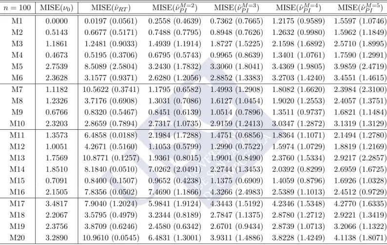
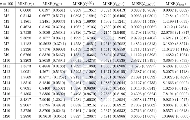
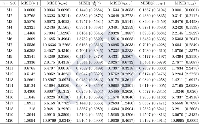
2.2.2 Simulation study

The effectiveness of the new selector, the plug–in rule, for selecting the smoothing parameter described in the previous section has been compared with the rule of thumb defined in (2.7), leasts squares cross–validation rule (2.9), likelihood cross–validation rule (2.10) and bootstrap method (2.12) through Monte Carlo experiments. A variety of circular distributions (von Mises, cardioid, various wrapped distributions and mixtures of them) displaying multimodality, skewness and/or peakedness have been tried (see Figure 2.2for plots and Appendix A for specific formulae). For illustration purposes, the models have been classified in four groups, according to their complexity: Simple models: circular uniform (M1); von Mises (M2); wrapped normal (M3); cardioid (M4); wrapped Cauchy (M5) and wrapped skew–normal (M6).

Two components models: von Mises mixtures (M7, M8 and M9); mixture of von Mises and wrapped Cauchy (M10).

Models with more than two components: von Mises mixtures with three components (M11, M12 and M13); von Mises mixture with four components (M14); mixture of wrapped Cauchy, wrapped normal, von Mises and wrapped skew–normal (M15); von Mises mixture with five components (M16).

Other complex models: mixture of cardioid and wrapped Cauchy (M17); mixture of von Mises (M18 and M19); mixture of two wrapped skew–normal and two wrapped Cauchy (M20).

Note that Simple models include unimodal models from von Mises distributions, with the circular uniform as a particular case. The wrapped Cauchy shows a highly peaked mode, whereas an asymmetric model is obtained with the wrapped skew–normal, as shown inPewsey(2006). The Two components models collect different mixtures of two von Mises distributions (with antipodal modes and combining different weights and centers) and a mixture of a von Mises and a wrapped