Testing parametric models in linear-directional
regression
Eduardo Garc´ıa-Portugu´
es
1,2,3,5Ingrid Van Keilegom
4Rosa M. Crujeiras
3Wenceslao Gonz´
alez-Manteiga
3Abstract
This paper presents a goodness-of-fit test for parametric regression models with scalar response and directional predictor, that is, a vector on a sphere of arbitrary dimension. The testing procedure is based on the weighted squared distance between a smooth and a parametric regression estimator, where the smooth regression estimator is obtained by a projected local approach. Asymptotic behavior of the test statistic under the null hypothesis and local alternatives is provided, jointly with a consistent bootstrap algorithm for application in practice. A simulation study illustrates the performance of the test in finite samples. The procedure is applied to test a linear model in text mining.
Keywords: bootstrap calibration, directional data, goodness-of-fit test, local linear regres-sion.
Running title: Testing in linear-directional regression.
1Department of Mathematical Sciences. University of Copenhagen (Denmark).
2The Bioinformatics Centre, Department of Biology. University of Copenhagen (Denmark).
3Department of Statistics and Operations Research. University of Santiago de Compostela (Spain). 4Institute of Statistics, Biostatistics and Actuarial Sciences. Universit´e catholique de Louvain (Belgium). 5Corresponding author. e-mail: [email protected].
1
Introduction
Directional data (data on a general sphere of dimension q) appear in a variety of contexts, the simplest one being provided by observations of angles on a circle (circular data). Direc-tional data is present in wind directions or animal orientation (Mardia and Jupp, 2000) and, recently, it has been considered in higher dimensional settings for text mining (Srivastava and Sahami, 2009). In order to identify a statistical pattern within a certain collection of texts, these objects may be represented by a vector on a sphere where each vector component gives the relative frequency of a certain word. From this vector-space representation, text classification can be performed (Banerjee et al., 2005), but other interesting problems such as popularity prediction could be tackled. For instance, a linear-directional regression model could be used to predict the popularity of articles in news aggregators, quantified by the number of comments or views (Tatar et al., 2012), based on the news contents.
When dealing with directional and linear variables at the same time, the joint behavior could be modeled by considering a flexible density estimator (Garc´ıa-Portugu´es et al., 2013). Nev-ertheless, a regression approach may be more useful, allowing at the same time for explaining a relation between the variables and for making predictions. Nonparametric regression es-timation methods for linear-directional models have been proposed by different authors. For example, Cheng and Wu (2013) introduced a general local linear regression method on manifolds and, quite recently, Di Marzio et al. (2014) presented a local polynomial method when both the predictor and the response are defined on spheres. Despite the flexibility of these estimators, in terms of interpretation of the results, purely parametric models may be more convenient. In this context, goodness-of-fit tests can be designed, providing a tool for assessing a certain parametric linear-directional regression model.
Goodness-of-fit tests for directional data, or including a directional component in the data generating process, have not been deeply studied. For the density case, Boente et al. (2014) provide a nonparametric goodness-of-fit test for directional densities and similar ideas are used by Garc´ıa-Portugu´es et al. (2015) for directional-linear densities. Except for the
ex-ploratory tool and lack-of-fit test for linear-circular regression developed by Deschepper et al. (2008) there are no other works in the regression context. The related Euclidean literature is extensive: the reader is referred to Hart (1997) for a comprehensive reference and to H¨ardle and Mammen (1993) and Alcal´a et al. (1999) for the most relevant works for this contribution.
This paper presents a goodness-of-fit test for parametric linear-directional regression mod-els. The test is constructed from a projected local regression estimator (Section 2). The asymptotic distribution of the test statistic, based on a weighted squared distance between the nonparametric and parametric fits, is obtained under a family of local alternatives con-taining the null hypothesis (Section 3). A bootstrap strategy, proved to be consistent, is proposed for the calibration of the test in practice. The performance of the test is checked for finite samples in a simulation study (Section 4) and the test is applied to assess a con-strained linear model for news popularity prediction in text mining (Section 5). An appendix contains the proofs of the main results, whereas technical lemmas and further information on the simulation study and data application are provided as Supporting Information (SI).
2
Nonparametric linear-directional regression
Let Ωq =
x ∈ Rq+1 : ||x|| = 1 denote the q-sphere in
Rq+1 and ωq denote both its
associated Lebesgue measure and its surface area,ωq = 2π
q+1 2 Γ q+1 2 . A directional density f satisfiesRΩ
qf(x)ωq(dx) = 1. From a sampleX1, . . . ,Xn of a random variable (rv)Xwith
density f, Hall et al. (1987) and Bai et al. (1988) introduced the kernel density estimator ˆ fh(x) = 1 n n X i=1 Lh(x,Xi), Lh(x,y) = ch,q(L)L 1−xTy h2 , x∈Ωq, (1)
where L is a directional kernel,h >0 is the bandwidth parameter and
ch,q(L)−1 =λh,q(L)hq =λq(L)hq(1 +
o
(1)) (2) with λh,q(L) =ωq−1 R2h−2 0 L(r)r q 2−1(2−rh2) q 2−1dr and λq(L) = 2 q 2−1ωq−1R∞ 0 L(r)r q 2−1dr.Assume that X is the covariate in the regression model
whereY is a scalar (response) rv,m is the regression function given by the conditional mean (m(x) =E[Y|X=x]), and σ2 is the conditional variance (σ2(x) =Var [Y|X=x]). Errors are collected by ε, a rv such that E[ε|X] = 0, E[ε2|X] = 1 and
E[|ε|3|X] and E[ε4|X] are
assumed to be bounded rv’s. Bothm, f : Ωq −→Rcan be extended from Ωq toRq+1\{0}by
considering a radial projection. This allows the consideration of easily tractable derivatives and the use of Taylor expansions.
A1. m and f are extended from Ωq to Rq+1\{0} by m(x) ≡ m(x/||x||) and f(x) ≡
f(x/||x||). mis three times andf is twice continuously differentiable andf is bounded away from zero.
Assumption A1 guarantees thatf and m are uniformly bounded in Ωq. More importantly,
the directional derivative of m (and f) in the direction x and evaluated at x is zero, i.e.,
xT∇m(x) = 0. This is a key fact on the construction of Taylor expansion ofm at Xi:
m(Xi) =m(x) +∇m(x)T(Xi−x) +O |Xi−x)2 =m(x) +∇m(x)T Iq+1−xxT (Xi−x) +O ||Xi−x|| 2 ≈β0+βT1B T x(Xi−x),
whereBx= (b1, . . . ,bq)(q+1)×q is theprojection matrix that completesx to an orthonormal
basis{x,b1, . . . ,bq}ofRq+1 and satisfiesBTxBx=Iq andBxBTx =
Pq
i=1bibTi =Iq+1−xxT,
with Iq the identity matrix of dimension q.
With this setting, β0 ∈ R captures the constant effect in m(x) while β1 ∈Rq contains the
linear effects of the projected gradient of m given by BT
x∇m(x). It should be noted that
the dimension of β1 is the adequate for the q-sphere Ωq, which would be q+ 1 if an usual
Taylor expansion in Rq+1 was performed. Theprojected local estimator atm(x) is obtained
as the weighted average of local constant (denoted by p= 0) or linear (p = 1) fits given by
β0 or β0 +βT1BTx(Xi −x), respectively. Given the sample (X1, Y1), . . . ,(Xn, Yn) from (3),
formulated as the weighted least squares problem min β∈Rq+1 n X i=1 Yi −β0−δp,1(β1, . . . , βq) T BTx(Xi−x) 2 Lh(x,Xi),
where δr,s is the Kronecker Delta. The solution to the minimization problem is given by
ˆ
β= XTx,pWxXx,p
−1
XTx,pWxY, (4)
where Y is the vector of observed responses, Wx is the diagonal weight matrix with i-th
entry Lh(x,Xi),Xx,1 is the design matrix with i-th row (1,(Xi−x)TBx) and Xx,0 =1 (1
stands for a vector of ones whose dimension is determined by the context). The projected local estimator at x is given by ˆβ0 = ˆmh,p(x) and is a weighted linear combination of the
responses (e1 is a null vector with one in the first component):
ˆ mh,p(x) =eT1 X T x,pWxXx,p −1 XT x,pWxY= n X i=1 Wnp(x,Xi)Yi, (5)
The next assumptions ensure that ˆmh,p is a consistent estimator of m:
A2. The conditional variance σ2 is uniformly continuous and bounded away from zero.
A3. L: [0,∞)→[0,∞) is a continuous and bounded function with exponential decay.
A4. The sequence of bandwidths h =hn is positive and satisfiesh→0 and nhq → ∞.
Assumptions A2 and A4 are usual assumptions for the multivariate local linear estimator (Ruppert and Wand, 1994). A3allows for the use of non-compactly supported kernels, such as the popular von Mises kernel L(r) = e−r.
Remark 1. The proposal of Di Marzio et al. (2014) for a local linear estimator ofmis rooted on a Taylor expansion of the sin and cos functions of the tangent-normal decomposition. This leads to an overparametrized design matrix ofq+ 2columns which makes XTx,pWxXx,p
exactly singular, a fact handled by the authors with a pseudo-inverse. It should be noted that Di Marzio et al. (2014)’s proposal and (5) present some remarkable differences: for the circular case, (5) corresponds to Di Marzio et al. (2009)’s proposal (with parametrization
κ≡1/h2), but Di Marzio et al. (2014) differs from the aforementioned reference. Although both estimators share the same asymptotics, (5) somehow offers a simpler construction and a more natural connection with previous proposals.
3
Goodness-of-fit test for linear-directional regression
Assuming that model (3) holds, the goal is to test if the regression function m belongs to the parametric class of functions MΘ ={mθ :θ ∈Θ⊂Rs}. This is equivalent to testing
H0 :m(x) =mθ0(x), for all x∈Ωq, versus H1 :m(x)6=mθ0(x), for some x∈Ωq,
with θ0 ∈ Θ known (simple hypothesis) or unknown (composite) and where for all holds
except for a set of probability zero and for some holds for a set of positive probability. The proposed statistic to test H0 compares the nonparametric estimator with a smoothed
parametric estimator inMΘ through a squared weighted norm:
Tn =
Z
Ωq
( ˆmh,p(x)− Lh,pmˆθ(x))2fˆh(x)w(x)ωq(dx)
where Lh,pm(x) =Pni=1Wnp(x,Xi)m(Xi) represents the local smoothing of the functionm
from measurements {Xi} n
i=1 and ˆθ denotes either the known parameter θ0 (simple
hypoth-esis) or a consistent estimator (composite hypothesis; see A6 below). An equivalent ex-pression forTn, useful for computational implementation, isTn =
R Ωq Pn i=1W p n(x,Xi)(Yi− mθˆ(Xi)) 2ˆ
fh(x)w(x)ωq(dx). This smoothing of the (possibly estimated) parametric
regres-sion function is included to reduce the asymptotic bias (H¨ardle and Mammen, 1993). Besides, in order to mitigate the effect of the difference between ˆmh,p and mθˆ in sparse areas of the
covariate, the squared difference is weighted by a kernel density estimate of X, namely ˆfh.
In addition, by the inclusion of ˆfh, the effects of the unknown density both on the
asymp-totic bias and variance are removed. Optionally, a weight functionw: Ωq −→[0,∞) can be
considered, for example, to restrict the test to specific regions of Ωq by an indicator function.
The limit distributions ofTn are analyzed under a family of local alternatives that contains
H0 as a particular case and is asymptotically close to H0:
H1P :m(x) =mθ0(x) +cng(x), for all x∈Ωq,
where mθ0 ∈ MΘ,g : Ωq −→R and cn is a positive sequence such that cn→0, for instance
cn= nh
q
2− 1
2. With this framework,H
1P becomesH0 wheng is such thatmθ0+c
−1
2
(g ≡0, for example) andH1 when the previous statement does not hold for a set of positive
probability. The following regularity conditions on the parametric estimation are required:
A5. mθ is continuously differentiable as a function of θ, and this derivative is also
contin-uous for x∈Ωq.
A6. UnderH0, there exists an √
n-consistent estimator ˆθ ofθ0,i.e. θˆ−θ0 =OP n
−1
2and
such that, under H1, ˆθ−θ1 =OP n
−12
for a certain θ1.
A7. The function g is continuous.
A8. Under H1P , the
√
n-consistent estimator ˆθ also satisfies ˆθ−θ0 =OP n
−12
.
Theorem 1 (Limit distributions of Tn). Under H1P, A1–A6 and A7–A8 if g 6≡0,
nhq2 T n− λq(L2)λq(L)−2 nhq Z Ωq σθ20(x)w(x)ωq(dx) ! d −→ ∞, c2 nnh q 2 → ∞, NR Ωqg(x) 2f(x)w(x)ω q(dx),2νθ20 , c2nnhq2 →δ, 0< δ <∞, N(0,2ν2 θ0), c 2 nnh q 2 →0, where σ2 θ0(x) = E[(Y −mθ0(X))
2|X=x] is the conditional variance under H
0 and νθ20 = Z Ωq σθ40(x)w(x)2ωq(dx)×γqλq(L)−4 Z ∞ 0 rq2−1 Z ∞ 0 ρq2−1L(ρ)ϕ q(r, ρ)dρ 2 dr, ϕq(r, ρ) = Lr+ρ−2(rρ)12 +Lr+ρ+ 2(rρ)12 , q= 1, R1 −1(1−θ 2)q−32 L r+ρ−2θ(rρ)12 dθ, q≥2, γq = 2−12, q= 1, ωq−1ω2q−22 3q 2−3, q≥2.
The convergence rate as well as the asymptotic bias and variance agree with the results in the Euclidean setting given by H¨ardle and Mammen (1993) and Alcal´a et al. (1999), except for the cancellation of the design density in the bias and variance, achieved by the inclusion of ˆfh in the test statistic. The use of a local estimator withp= 0 orp= 1 does not affect the
seen in the SI). Finally, the general complex structure of the asymptotic bias and variance turns much simpler with the von Mises kernel:
ν2 = Z Ωq σ4(x)w(x)2ωq(dx)×(8π)− q 2, λq(L2)λq(L)−2 = 2π 1 2−q.
3.1
Bootstrap calibration
The distribution of Tn under H0 can be approximated by the one of its bootstrapped
version Tn∗, which can be arbitrarily well approximated by Monte Carlo by generating bootstrap samples. Under H0, the bootstrap responses are obtained from the parametric
fit and bootstrap errors that imitate the conditional variance by a wild bootstrap proce-dure: Yi∗ = mθˆ(Xi) + ˆεiVi∗, where ˆεi = Yi − mθˆ(Xi) and the variables V1∗, . . . , V
∗
n are
independent from the observed sample and iid with E[Vi∗] = 0, Var [Vi∗] = 1 and fi-nite third and fourth moments. A common choice is considering a binary variable with
PVi∗ = (1−
√
5)/2 = (5 +√5)/10 and PVi∗ = (1 +√5)/2 = (5−√5)/10, which cor-responds to the golden section bootstrap. The test in practice for the composite hypothesis is summarized in the next algorithm (if the simple is considered, set θ0 = ˆθ= ˆθ
∗
).
Algorithm 1 (Test in practice). Consider {(Xi, Yi)} n
i=1 a sample from (3). To test H0, set
a bandwidth h and (optionally) a weight function w and proceed as follows: i. Compute θˆ, εˆi =Yi−mθˆ(Xi) and Tn= R Ωq Pn i=1W p n(x,Xi)ˆεi 2ˆ fh(x)w(x)ωq(dx).
ii. Bootstrap resampling. For b= 1, . . . , B: (a) Obtain {(Xi, Yi∗)} n i=1, where Y ∗ i =mθˆ(Xi) + ˆεiVi∗ and compute θˆ ∗ as in i. (b) ComputeTn∗b =RΩ q Pn i=1W p n(x,Xi)ˆε∗i 2ˆ fh(x)w(x)ωq(dx)withεˆi ∗ =Yi∗−mθˆ∗(Xi).
iii. Approximate thep-value by B1 PB
b=11{Tn≤Tn∗b}.
In order to prove the consistency of the resampling mechanism, that is, thatTn∗ has the same asymptotic distribution of Tn, a bootstrap analogue of assumptionA6 is required:
A9. The estimator ˆθ∗ computed from{(Xi, Yi∗)} n i=1 is such that ˆθ ∗ −θˆ =OP∗ n− 1 2, where
From this assumption and Theorem 1 it follows that the probability distribution function (pdf) ofTn∗, conditionally on the sample, converges always in probability to a Gaussian pdf, which is the same asymptotic pdf of Tn if H0 holds.
Theorem 2(Bootstrap consistency). UnderA1–A6andA9and conditionally on{(Xi, Yi)}ni=1,
nhq2 T∗ n − λq(L2)λq(L)−2 nhq Z Ωq σ2θ1(x)w(x)ωq(dx) ! d −→ N 0,2νθ21
in probability. If the null hypothesis holds, then θ1 =θ0.
4
Simulation study
The finite sample performance of the goodness-of-fit test is explored in four simulation scenarios, labeled S1 to S4. Their associated parametric regression models are shown in Figure 1 with the following codification: the radius from the origin represents the response
m(x) for an x direction, resulting in a distortion from a perfect circle or sphere. The design densities of the scenarios are taken from Garc´ıa-Portugu´es (2013), the noise is either heteroskedastic (S1 and S2) or homocedastic (S3 and S4) and two different deviations (for S1–S2 and for S3–S4) are considered. The tests based on the projected local constant and linear estimators are compared with M = 1000 Monte Carlo trials and B = 1000 bootstrap replicates, under H0 and H1, for a grid of bandwidths and with n = 100 and q = 1,2,3.
Parametric estimation is done by nonlinear least squares, which is justified by their simplicity and asymptotic normality (Jennrich, 1969), hence satisfyingA6. For the sake of brevity, only a coarse grained description of the scenarios and a selected output of the study is provided here. The reader is referred to the SI for the complete report.
[Figure 1 around here]
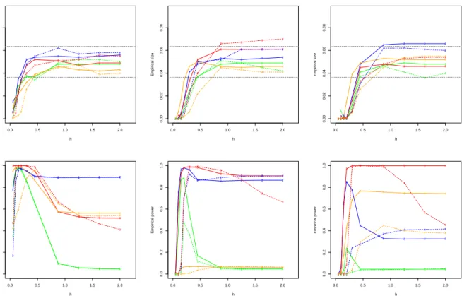
The empirical sizes of the goodness-of-fit tests are shown using the so called significance trace (Bowman and Azzalini, 1997), i.e., the curve of percentages of empirical rejections for different bandwidths. As shown in Figure 2, except for very small bandwidths that result in a conservative test, the significance level is stabilized around the 95% confidence band
for the nominal level α = 0.05, for the different scenarios and dimensions. The power is satisfactory, given that the proposed tests succeed in detecting the mild deviations from the null hypotheses. Despite the fact that the test based on the local linear estimator (p = 1) provides a better power for large bandwidths in certain scenarios, the overall impression is that the test with p = 0 is hard to beat: the powers with p = 0 and p = 1 are almost the same for low dimensions, whereas as the dimension increases the local constant estimator performs better for a wider range of bandwidths. This effect could be explained by the spikes that local linear regression tends to show in the boundaries of the support (design densities of S3 and S4), which become more important as the dimension increases. The lower power for S1 and S4 is due to deviations happening in areas with low density or high variance.
[Figure 2 around here]
5
Application to text mining
In different applications within text mining, it is quite common to consider acorpus (collec-tion of documents) and to determine the so-called vector space model: a corpusd1, . . . ,dn is
codified by the set of vectors{(di1, . . . , diD)} n
i=1 (the document-term matrix) with respect to
a dictionary (or a bag of words) {w1, . . . , wD}, such thatdij represents the frequency of the
dictionary’s j-th word in the document di. Usually, a normalization of the document-term
matrix is performed to remove length distortions and map documents with similar contents, albeit different lengths, into close vectors. If the Euclidean norm is used for this, then the documents can then be regarded as points in ΩD−1 providing a set of directional data.
The corpus that is analyzed in this application was acquired from the news aggregator Slash-dot (wwww.slashdot.org). This website publishes summaries of news about technology and science that are submitted and evaluated by users. Each news entry includes a title, a sum-mary with links to other related news and a discussion thread gathering users comments. The goal is to test a linear model that takes as a predictor the topic of the news (a directional variable in ΩD−1) and as a response the log-number of comments. This is motivated by the
that, in text classifications, it has been checked that non-linear classifiers hardly provide any advantage with respect to linear ones (Joachims, 2002). After a data preprocessing process (using Meyer et al. (2008); see SI), the n= 8121 news collected from 2013 were represented in a document term matrix formed by D= 1508 words.
In order to construct a plausible linear model, a preliminary variable selection was per-formed using LASSO regression with (tuning) parameter λ selected by an overpenalized
three standard error rule (Hastie et al., 2009). After removing some extra variables by using a backward stepwise method with BIC, a fitted vector ˆη∈RD with d= 77 non-zero entries
is obtained. The test is applied to check the null hypothesis of a candidate linear model with coefficient η constrained to be zero except in these previously selected d words, that is H0 : m(x) = c+ηTx, with η subject to Aη = 0 for an adequate choice of the matrix
A(D−d)×D. The significance trace of the test (with p = 0; p = 1 was not implemented due
to its higher cost and to computational limitations) presents a minimum p-value of 0.12, hence showing no evidence to reject the linear model for a wide grid of bandwidths. Figure 3 displays a graphical summary of the fitted linear model. As it can be seen, news where stemmed words like “kill”, “climat”, “polit” appear have a strong positive impact on the number of comments, since these news are likely more controversial and generate broader discussions. On the other hand, scientific related words like “mission”, “abstract” or “lab” have a negative impact, as they tend to raise more objective and higher specific discussions. Experiments were conducted with a model of d = 50 non-zero coefficients chosen with a higher overpenalization, showing a strong rejection of the null hypothesis.
[Figure 3 around here]
Acknowledgments
We thank professors David E. Losada for his guidance in the data application and Ir`ene Gij-bels for her useful theoretical comments. This research was supported by Project MTM2008– 03010 from the Spanish Ministry of Science and Innovation, Project 10MDS207015PR from
Direcci´on Xeral de I+D of the Xunta de Galicia, by IAP research network grant nr. P7/06 of the Belgian government (Belgian Science Policy), by the European Research Council un-der the European Community’s Seventh Framework Programme (FP7/2007–2013) / ERC Grant agreement No. 203650, and by the contract “Projet d’Actions de Recherche Con-cert´ees” (ARC) 11/16–039 of the “Communaut´e fran¸caise de Belgique” (granted by the “Acad´emie universitaire Louvain”). Work of the first author has been supported by a grant from Fundaci´on Barri´e and FPU grant AP2010–0957 from the Spanish Ministry of Edu-cation. Authors gratefully acknowledge the computational resources used at the CESGA Supercomputing Center and valuable suggestions by three anonymous referees.
Supporting Information
Supporting information available online contains the technical lemmas used and further information on the simulation study and text mining application.
References
Alcal´a, J. T., Crist´obal, J. A., and Gonz´alez-Manteiga, W. (1999). Goodness-of-fit test for linear models based on local polynomials. Statist. Probab. Lett., 42(1):39–46.
Bai, Z. D., Rao, C. R., and Zhao, L. C. (1988). Kernel estimators of density function of directional data. J. Multivariate Anal., 27(1):24–39.
Banerjee, A., Dhillon, I. S., Ghosh, J., and Sra, S. (2005). Clustering on the unit hypersphere using von Mises-Fisher distributions. J. Mach. Learn. Res., 6:1345–1382.
Boente, G., Rodr´ıguez, D., and Gonz´alez-Manteiga, W. (2014). Goodness-of-fit test for directional data. Scand. J. Stat., 41(1):259–275.
Bowman, A. W. and Azzalini, A. (1997). Applied smoothing techniques for data analysis: the kernel approach with S-Plus illustrations. Oxford Statistical Science Series. Clarendon Press, Oxford.
Cheng, M.-Y. and Wu, H.-T. (2013). Local linear regression on manifolds and its geometric interpretation. J. Amer. Statist. Assoc., 108(504):1421–1434.
de Jong, P. (1987). A central limit theorem for generalized quadratic forms. Probab. Theory Related Fields, 75(2):261–277.
Deschepper, E., Thas, O., and Ottoy, J. P. (2008). Tests and diagnostic plots for detecting lack-of-fit for circular-linear regression models. Biometrics, 64(3):912–920.
Di Marzio, M., Panzera, A., and Taylor, C. C. (2009). Local polynomial regression for circular predictors. Statist. Probab. Lett., 79(19):2066–2075.
Di Marzio, M., Panzera, A., and Taylor, C. C. (2014). Nonparametric regression for spherical data. J. Amer. Statist. Assoc., 109(506):748–763.
Fan, J. and Gijbels, I. (1996). Local polynomial modelling and its applications, volume 66 of
Monographs on Statistics and Applied Probability. Chapman & Hall, London.
Garc´ıa-Portugu´es, E. (2013). Exact risk improvement of bandwidth selectors for kernel density estimation with directional data. Electron. J. Stat., 7:1655–1685.
Garc´ıa-Portugu´es, E., Crujeiras, R. M., and Gonz´alez-Manteiga, W. (2013). Kernel density estimation for directional-linear data. J. Multivariate Anal., 121:152–175.
Garc´ıa-Portugu´es, E., Crujeiras, R. M., and Gonz´alez-Manteiga, W. (2015). Central limit theorems for directional and linear data with applications. Statist. Sinica, 25:1207–1229. Hall, P., Watson, G. S., and Cabrera, J. (1987). Kernel density estimation with spherical
data. Biometrika, 74(4):751–762.
H¨ardle, W. and Mammen, E. (1993). Comparing nonparametric versus parametric regression fits. Ann. Statist., 21(4):1926–1947.
Hart, J. D. (1997). Nonparametric smoothing and lack-of-fit tests. Springer Series in Statis-tics. Springer-Verlag, New York.
Hastie, T., Tibshirani, R., and Friedman, J. (2009). The elements of statistical learning. Springer Series in Statistics. Springer, New York, second edition.
Jennrich, R. I. (1969). Asymptotic properties of non-linear least squares estimators. Ann. Math. Statist., 40(2):633–643.
Joachims, T. (2002).Learning to classify text using support vector machines: Methods, theory and algorithms, volume 668 of Kluwer International Series in Engineering and Computer Science. Kluwer Academic Publishers, Boston.
Mardia, K. V. and Jupp, P. E. (2000). Directional statistics. Wiley Series in Probability and Statistics. John Wiley & Sons, Chichester, second edition.
Meyer, D., Hornik, K., and Feinerer, I. (2008). Text mining infrastructure in R. J. Stat. Softw., 25(5):1–54.
Ruppert, D. and Wand, M. P. (1994). Multivariate locally weighted least squares regression.
Ann. Statist., 22(3):1346–1370.
Srivastava, A. N. and Sahami, M., editors (2009). Text mining: classification, clustering, and applications. Chapman & Hall/CRC Data Mining and Knowledge Discovery Series. CRC Press, Boca Raton.
Tatar, A., Antoniadis, P., De Amorim, M. D., and Fdida, S. (2012). Ranking news articles based on popularity prediction. In Proceedings of the 2012 International Conference on Advances in Social Networks Analysis and Mining (ASONAM 2012), pages 106–110. IEEE.
A
Proofs of the main results
Proof of Theorem 1. The proof follows the steps of H¨ardle and Mammen (1993) and Alcal´a et al. (1999). Tn can be separated into three addends by adding and subtracting the true
smoothed regression function Tn= (Tn,1+Tn,2−2Tn,3)(1 +
o
P(1)), whereTn,1 = Z Ωq n X i=1 Wnp(x,Xi) (Yi−mθ0(Xi)) 2 f(x)w(x)ωq(dx),
Tn,2 = Z Ωq (Lh,p(mθ0 −mθˆ) (x)) 2 f(x)w(x)ωq(dx), Tn,3 = Z Ωq ( ˆmh,p(x)− Lh,pmθ0(x))Lh,p(mθ0 −mθˆ) (x)f(x)w(x)ωq(dx),
because i of Lemma 4. The proof is divided into the analysis of each addend.
Terms Tn,2 and Tn,3. By a Taylor expansion on mθ(x) as a function ofθ (see A5),
Tn,2 = Z Ωq ˆ θ−θ0 T Lh,p(OP(1)) (x) 2 f(x)w(x)ωq(dx) =OP n −1 ,
because of the boundedness of ∂mθ(x)
∂θ for x∈Ωq, A6 and A8. On the other hand,
Tn,3 =OP n −1 2 Z Ωq ( ˆmh,p(x)− Lh,pmθ0(x))f(x)w(x)ωq(dx) =OP n −1 ,
because of the previous considerations and i from Lemma 6. As a consequence, by A3 it happens that nhq2Tn,3 −→p 0 and nh
q
2Tn,2 −→p 0.
Term Tn,1. Tn,1 is dealt with ˜Lh(x,Xi) = nhqλ 1 q(L)f(x)L 1−xTXi h2 from Lemma 5: Tn,1 = Z Ωq n X i=1 ˜ Lh(x,Xi) (1 +
o
P(1)) (Yi−mθ0(Xi)) 2 f(x)w(x)ωq(dx) =Ten,1(1 +o
P(1)).Now it is possible to split Ten,1 = Te (1) n,1 +Te (2) n,1 + 2Te (3) n,1 by recalling that Yi − mθ0(Xi) =
σ(Xi)εi+cng(Xi) by (3) and H1P. Specifically, under H1P the conditional variance can be
expressed as σ2(x) =
E(Y −mθ0(X)−cng(X)
2
|X =x =σ2
θ0(x)(1 +
o
(1)), uniformly inx∈Ωq since g and σθ0 are continuous and bounded by A2 and A7. Therefore:
e Tn,(1)1 = Z Ωq n X i=1 ˜ Lh(x,Xi)σ(Xi)εi 2 f(x)w(x)ωq(dx), e Tn,(2)1 =c2n Z Ωq n X i=1 ˜ Lh(x,Xi)g(Xi) 2 f(x)w(x)ωq(dx), e Tn,(3)1 =cn Z Ωq n X i=1 n X j=1 ˜ Lh(x,Xi) ˜Lh(x,Xj)σ(Xi)εig(Xj)f(x)w(x)ωq(dx).
By results ii and iii of Lemma 6, the behavior of the two last terms is
nhq2Te(2) n,1 =nh q 2c2 n Z Ωq g(x)2f(x)w(x)ωq(dx)(1 +
o
P(1)) and nh q 2Te(3) n,1 =o
P(1). (6)If c2 nnh q 2 → ∞, then nh q 2Te(2)
n,1 → ∞, yielding a degenerate asymptotic distribution. If
c2 nnh q 2 → 0, then nh q 2Te(2)
n,1 =
o
P(1). For these reasons, cn = nhq
2− 1
2 is assumed from now
on. For the first addend, let consider
e Tn,(1)1 = Z Ωq n X i=1 ˜ Lh(x,Xi)σ(Xi)εi 2 f(x)w(x)ωq(dx) + Z Ωq X i6=j ˜ Lh(x,Xi) ˜Lh(x,Xj)σ(Xi)σ(Xj)εiεjf(x)w(x)ωq(dx) =Te (1a) n,1 +Te (1b) n,1 .
From result iv of Lemma 6 and because σ2(x) =σ2
θ0(x)(1 +
o
(1)) uniformly, nhq2Te(1a) n,1 = λq(L2)λq(L)−2 hq2 Z Ωq σ2θ0(x)w(x)ωq(dx)(1 +o
(1)) +o
P(1). The asymptotics of Te (1b)n,1 are obtained checking the conditions of Theorem 2.1 in de Jong
(1987): a) E[Wijn+Wjin|Xi] = 0, 1 ≤ i < j ≤ n; b) Var [Wn] → v2; c) max1≤i≤nPnj=1
Var [Wijn]
v−2 →0;d) E[Wn4]v−4 →3. To that end, let denote
Wijn =δi,jnh q 2 Z Ωq ˜ Lh(x,Xi) ˜Lh(x,Xj)σ(Xi)σ(Xj)εiεjf(x)w(x)ωq(dx). Then, nhq2Te(1b) n,1 = Wn = P
i6=jWijn and the rv’s on which Wijn depends are (Xi, εi) and
(Xj, εj). a) is easily seen to hold by E[ε|X] = 0 and the tower property, which implies that
E[Wijn] = 0. Because of this, the fact that Wijn=Wjin and Lemma 2.1 in de Jong (1987),
Var [Wn] =E X i6=j Wijn 2 = 2E X i6=j Wijn2 = 2n(n−1)EWijn2 . (7)
Then, byv in Lemma 6 and the fact thatσ2(x) =σθ20(x)(1+
o
(1)),EWijn2 =n−2νθ20(1 +o
(1)) and as a consequenceVar [Wn]→2νθ20. Conditionc) follows easily:max 1≤i≤n n X j=1 Var [Wijn] v−2 ≤ max 1≤i≤nn −1ν2 θ0(1 +
o
(1)) (2νθ20)−1 = (2n)−1(1 +o
(1))→0.To check d), note that E[W4
n] can be split in the following form in virtue of Lemma 2.1 in
de Jong (1987), as H¨ardle and Mammen (1993) stated:
EWn4 = 8X i,j 6 = EWijn4 + 12X i,j,k,l 6 = EWijn2 Wkln2 + 48X i,j,k 6 = EWijnWikn2 Wjkn
+ 192 X
i,j,k,l
6
=
E[WijnWjknWklnWlin], (8)
whereP6= stands for the summation over allpairwise different indexes (i.e., such that i6=j
for their associatedWijn). Byv of Lemma 6,E
W4 ijn =O((n4hq)−1), E[WijnWjknWklnWlin] =
O(n−4h2q) and E[WijnWikn2 Wjkn] =O(n−4). Therefore, by (7) and (8),
EWn4 = 12X i6=j X k6=l EWijn2 W 2 kln +
o
(1) = 32X i6=j EWijn2 2 +o
(1) = 3Var [Wn]2+o
(1) and by A4, E[W4n] = 3Var [Wn]2+
o
(1), sod) is satisfied, having thatnhq2Te(1b)
n,1
d
−→ N 0,2νθ20. (9)
Using the decomposition for Tn with the dominant termsTe
(1a) n,1 , Te (1b) n,1 and Te (2) n,1, it holds nhq2T n= λq(L2)λq(L)−2 hq2 Z Ωq σθ20(x)w(x)ωq(dx) +nh q 2Te(1b) n,1 + Z Ωq g(x)2f(x)w(x)ωq(dx) (1 +
o
P(1))and the limit distribution follows by Slutsky’s theorem and (9).
Proof of Theorem 2. Analogously as in Theorem 1, Tn∗ =Tn,∗1+Tn,∗2−2Tn,∗3.
Terms Tn,∗2 and Tn,∗3. By A9 it is seen that nhq2T∗
n,2 p∗ −→ 0 and nhq2T∗ n,3 p∗ −→ 0, where the convergence is stated in the probability law P∗ that is conditional on the sample.
Term Tn,∗1. By ˆεiVi∗ = (Yi−mˆθ(Xi))Vi∗ the dominant term can be split into
Tn,∗1 = Z Ωq n X i=1 (Wnp(x,Xi) ˆεiVi∗) 2 ˆ fh(x)w(x)ωq(dx) + Z Ωq X i6=j Wnp(x,Xi)Wnp(x,Xj) ˆεiVi∗εˆjVj∗fˆh(x)w(x)ωq(dx) = T ∗(1) n,1 +T ∗(2) n,1 .
From result i of Lemma 7, the first term is
nhq2T∗(1) n,1 = λq(L2)λq(L)−2 hq2 Z Ωq σ2θ1(x)w(x)ωq(dx)(1 +
o
P(1)) +o
P∗(1), (10)so the dominant term isTn,∗(2)1 , whose asymptotic behavior is obtained using Theorem 2.1 in de Jong (1987) conditionally on the sample. For that aim, let denote
Wijn∗ =δi,jnh q 2 Z Ωq Wnp(x,Xi)Wnp(x,Xj) ˆεiVi∗εˆjVj∗fˆh(x)w(x)ωq(dx).
Then,nhq2T∗(2) n,1 =W ∗ n = P i6=jW ∗
ijn and the rv’s on whichW
∗
ijndepends are nowV
∗
i andV
∗
j .
Condition a) follows immediately by the properties of the Vi∗’s: E∗Wijn∗ +Wjin∗ |Vi∗ = 0. On the other hand, analogously to (7),
Var∗[Wn∗] = 2 X i6=j E∗Wijn∗2 = 2n2hqX i6=j " Z Ωq Wnp(x,Xi)Wnp(x,Xj) ˆεiεˆjfˆh(x)w(x)ωq(dx) #2
and by result ii of Lemma 7, Var∗[Wn∗] −→p 2νθ21, resulting in the verification of c) in probability. Condition d) is checked using the same decomposition for E∗W∗4
n
and the results collected inii of Lemma 7. Hence E∗
W∗4
n
= 3Var∗[Wn∗]2+
o
P(1) and d) is satisfied in probability, from which it follows that, conditionally on {(Xi, Yi)}n
i=1 the pdf of nh
q
2T∗(2)
n,1
converges in probability to the pdf of N(0,2ν2
θ1), that is: nhq2T∗(2) n,1 d −→ N 0,2νθ2 1 in probability. (11)
Using the decomposition of Tn∗, (11) and applying Slutsky’s theorem:
nhq2T∗ n = λq(L2)λq(L)−2 hq2 Z Ωq σ2θ 1(x)w(x)ωq(dx) +nh q 2T∗(2) n,1 (1 +
o
P(1)) +o
P∗(1). −4 −2 0 2 4 −4 −2 0 2 4 −4 −2 0 2 4 −4 −2 0 2 4Figure 1: From left to right: parametric regression models for scenarios S1 to S4, for circular and spherical cases. Color shading represents the distance from the origin of the regression surface.
1 1 11 1 1 1 1 1 1 0.0 0.5 1.0 1.5 2.0 0.00 0.02 0.04 0.06 0.08 h Empir ical siz e 2 2 2 2 2 2 2 2 2 2 3 3 3 3 3 3 3 3 3 3 4 4 4 4 4 4 4 4 4 4 1 1 1 1 1 1 1 1 1 1 2 2 2 2 2 2 2 2 2 2 3 3 3 3 3 3 3 3 3 3 44 4 4 4 4 4 4 4 4 1 11 1 1 1 1 1 1 1 0.0 0.5 1.0 1.5 2.0 0.00 0.02 0.04 0.06 0.08 h Empir ical siz e 2 2 2 2 2 2 2 2 2 2 3 3 3 3 3 3 3 3 3 3 4 4 4 4 4 4 4 4 4 4 1 1 11 1 1 1 1 1 1 2 2 2 2 2 2 2 2 2 3 3 3 3 3 3 3 3 3 4 44 4 4 4 4 4 4 1 1 1 1 1 1 1 1 1 1 0.0 0.5 1.0 1.5 2.0 0.00 0.02 0.04 0.06 0.08 h Empir ical siz e 2 2 2 2 2 2 2 2 2 2 3 3 3 3 3 3 3 3 3 3 4 44 4 4 4 4 4 4 4 1 1 1 1 1 1 1 1 1 2 2 2 2 2 2 2 2 2 3 3 3 3 3 3 3 3 3 4 4 4 4 4 4 4 4 4 1 11 1 1 1 1 1 1 1 0.0 0.5 1.0 1.5 2.0 0.0 0.2 0.4 0.6 0.8 1.0 h Empir ical po w er 2 2 2 2 2 2 2 2 2 2 3 3 3 3 3 3 3 3 3 3 4 4 4 4 4 4 4 4 4 4 1 1 11 1 1 1 1 1 1 2 2 22 2 2 2 2 2 2 3 3 3 3 3 3 3 3 3 3 4 4 4 4 4 4 4 4 4 4 1 1 11 1 1 1 1 1 1 0.0 0.5 1.0 1.5 2.0 0.0 0.2 0.4 0.6 0.8 1.0 h Empir ical po w er 2 2 22 2 2 2 2 2 2 3 3 3 3 3 3 3 3 3 3 4 4 44 4 4 4 4 4 4 1 11 1 1 1 1 1 1 1 2 2 2 2 2 2 2 2 2 3 3 3 3 3 3 3 3 3 4 4 4 4 4 4 4 4 4 1 1 1 1 1 1 1 1 1 1 0.0 0.5 1.0 1.5 2.0 0.0 0.2 0.4 0.6 0.8 1.0 h Empir ical po w er 2 2 2 2 2 2 2 2 2 2 33 3 3 3 3 3 3 3 3 4 4 4 4 4 4 4 4 4 4 1 1 11 1 1 1 1 1 2 2 2 2 2 2 2 2 2 3 3 3 3 3 3 3 3 3 4 4 4 4 4 4 4 4 4
Figure 2: Empirical sizes (first row) and powers (second row) for significance level α = 0.05 for the different scenarios, withp= 0 (solid line) andp= 1 (dashed line). From left to right: columns represent dimensions q = 1,2,3 with sample size n = 100. Green, blue, red and orange colors correspond to scenarios S1 to S4, respectively.
Figure 3: Stems of the 30 largest coefficients (in absolute value) of the fitted constrained linear model. Green and red colors account for positive and negative impacts on news popularity, respec-tively, whereas the size of the stem is proportional to the magnitude of its coefficient. The linear model has an R2 = 0.25 and the significances of each coefficient are lower than 0.002.