Re-Interpreting the Application of Gabor Filters
as a Manipulation of the Margin in Linear
Support Vector Machines
Ahmed Bilal Ashraf, Simon Lucey, Tsuhan Chen
Abstract—Linear filters are ubiquitously used as a pre-processing step for many classification tasks in computer vision. In particular, applying Gabor filters followed by a classification stage, such as a support vector machine (SVM), is now common practice in computer vision applications like face identity and expression recognition. A fundamental problem occurs, however, with respect to the high dimensionality of the concatenated Gabor filter responses in terms of memory requirements and computational efficiency during training and testing. In this paper we demonstrate how the pre-processing step of applying a bank of linear filters can be reinterpreted as manipulating the type of margin being maximized within the linear SVM. This new interpretation leads to sizable memory and computational advantages with respect to existing approaches. The re-interpreted formulation turns out to be indpendent of the number of filters, thereby allowing to examine the feature spaces derived from arbitrarily large number of linear filters, a hitherto untestable prospect. Further, this new interpretation of filter banks gives new insights, other than the often cited biological motivations, into why the pre-processing of images with filter banks, like Gabor filters, improves classification performance.
Index Terms—Gabor filters, support vector machine, maximum margin, expression recognition
✦
1
I
NTRODUCTIONLinear filters are often used to extract useful feature repre-sentations for classification problems in computer vision. One particular filter, based on the seminal work of Gabor [1], that has received attention in the vision community are Gabor wavelets due to their biological relevance and computational properties [2], [3], [4], [5]. The employment of a concatenation of Gabor filter responses, as a pre-processing step, before learning a classifier has found particular success in face identity [6], [7] and expression [8], [9] recognition when compared to learning those classifiers with original appearance features/pixels. However, a fundamental problem with these methods is the inherently large memory and computational overheads required for training and testing in the over-complete Gabor domain. As a result many approximations have been proposed in literature to circumvent this prob-lem [6], [7], [8], [10]. Even with these approximations, the sheer size of the over-complete Gabor domain representation limits the number of filters and the size of images that can be employed during the learning of most practical classifiers.
In this paper we present a method that is able to circumvent the need for any of these approximations when learning a linear support vector machine (SVM). Our method is inspired by some of the recent work of Shivaswamy and Jebara [11] concerning what “type” of margin should be maximized during the estimation of a maximum margin classifier such as an SVM. In this work Shivaswamy and Jebara discussed the importance of selecting the “correct” kind of margin when learning an SVM and how maximizing a margin based on Euclidean distance might not always be the best choice in terms of classifier generalization. In our proposed work, we demonstrate how the application of a bank of filters to a set
of training image data, whose high dimensional concatenated filter responses are then used to learn a linear SVM with a Eu-clidean distance margin, can be viewed as learning an SVM in the original low dimensional appearance space with a weighted Euclidean distance margin. This equivalence opens the door to the exploration of image resolutions and filter bank sizes previously unimaginable as the computational and memory requirements of learning the SVM are now independent of the number of filter banks. Our key contributions in this paper are as follows,
• Exploiting Parseval’s relation [12] (dot products are con-served between spatial and Fourier domains) we demon-strate that learning an SVM that maximized the Euclidean distance margin of Gabor pre-processed images can be reinterpreted as learning an SVM that maximizes the weighted Euclidean distance margin of the raw images in the Fourier domain (Section5).
• Demonstrate how to represent a complex 2D-DFT image as a real vector such that the inner product between these real-vectors is equivalent to the complex inner product of the Fourier representation. Based on this equivalence, conventional linear SVM packages can be employed for learning that can only handle real training vectors without any need to re-writing or expanding code (Section5.1). • Describe how the linear SVM learnt in the Fourier
domain can obtain an equivalent linear SVM in the original appearance domain without the need for any pre-processing filtering or 2D-DFT (Section5.2).
• We apply our novel computationally efficient framework to the challenging task of action unit detection on the Cohn-Kanade facial action database [13] exploring pre-viously impractical numbers of filter banks and filter
response resolutions. We additionally demonstrate that using the full resolution filter responses significantly outperforms previous approaches [7] that downsample the responses (Section 6).
We restrict our experiments in this paper solely to facial expression recognition, as the application of Gabor filters followed by an SVM is now considered one of the leading methods [8], [9] in terms of performance. Our approach, however, is not restricted to expression recognition with the approach outlined in this paper being applicable to many computer vision problems.
2
T
HEP
ROBLEMHitherto, a fundamental problem associated with the applica-tion of pre-processing linear filter banks (like Gabor) to an image before classification is the large memory and compu-tational overheads incurred, during training and testing, from the now overcomplete filter-based representation of that image. The significance of these additional memory requirements can be realized through a simple thought experiment where we apply a bank of 9×81 Gabor filters to a modest size image of48×48pixels, as originally espoused in [9] for the task of facial expression recognition. The application of 9×8 Gabor filters results in 9×8×48×48 = 165,888 features. If we have 10,000 images in our training set, this would require approximately6.17Gb of storage assuming the responses are stored as floats. If we were to push the bounds on our system and employ slightly larger images of say100×100pixels this would now require a very demanding 26.82 Gb of memory storage. If we were to further push the bounds of performance and entertain the employment of a 128×128bank of Gabor filters we would now require a very impractical 5.96 Tb of storage to train our classifier.
If one was to adopt a filter specific sampling strategy of the responses, based on the spectral characteristics of each filter, one could lessen the memory overhead of this na¨ıve approach, without information loss, by sampling each response according to the filter’s Nyquist rate [12]. However, even with this more sophisitcated sampling strategy, one is still left with the realization that memory storage constraints directly influence the number and type of filters one can employ in any practical learning scenario. As a result of this inherent computation and memory problem the employment of banks of Gabor filters larger than 9×8 have been seldom reported in literature. Even for smaller filter bank sizes authors in literature have resorted to methods for approximating the full response vectors such as: (i) a lossy downsampling of filter responses [7], (ii) employing filter responses at certain fiducial positions within the image [6], (iii) the employment of feature selection methods to select the most discriminative filter responses [8], and most recently (iv) where individual classifiers are learnt for each filter response and a fusion strategy employed to combine the outputs in a synergistic manner [10].
1. Gabor filters are often referred to as a bank of x×yfilters where x
refers to the number of scales andyrefers to the number of orientations
The central purpose of this paper is to report a method that requires no approximation to the full resolution responses without any additional memory overhead, and demonstrate that the preservation of these full resolution responses leads to improved performance over well known approximation methods [7].
3
G
ABORF
ILTERR
EPRESENTATIONSInspired by previous breakthroughs in quantum theory Ga-bor [1] derived an uncertainty relation for information in the mid 1940s. Gabor elaborated a quantum theory of information that consigns signals to regions of an information diagram whose coordinates are time and frequency and whose minimal area (a product of frequency bandwidth and temporal duration) is governed by an “uncertainty principle” similar to the one found in quantum physics. He demonstrated that this quantile grain of information can be redistributed in shape but not re-duced in area, and that the general family of signals, which are commonly referred to now as Gabor filters, that achieve this smallest possible grain size are Gaussian modulated sinusoids. In the 1980s it was demonstrated [2], [3], [4], [5] how these family of signals could be expanded to handle 2D spatial signals and how they could be related to wavelet theory. In this same body of work it was demonstrated that these filters were similar to the 2D receptive field profiles of the mammalian cortical simple cells, and have desirable properties in spatial locality and orientation selectivity.
In the 2D spatial domain, a Gabor wavelet is a complex exponential modulated by a Gaussian,
gω,θ(x, y) = 1 2πσ2exp{− x02+y02 2σ2 +jωx 0 } (1)
where x0 = xcos(θ) +ysin(θ), y0 =−xsin(θ) +ycos(θ),
x and y denote the pixel positions, ω represents the centre frequency,θ represents the orientation of the Gabor wavelet, while σdenotes the standard deviation of the Gaussian func-tion. Please refer to [5] on strategies for spacing the filters in the 2D spatial frequency domain for a fixed number of scales and orientations. Given a N dimensional vectorized input image x and the vectorized P ×Q 2D filter gω,θ =
[gω,θ(1,1), . . . , gω,θ(P, Q)]T one can obtain the N
dimen-sional vector response,
ˆrω,θ= ˆx◦gˆω,θ (2)
where gˆω,θ, ˆx and ˆrω,θ2 are the vectorized complex 2D
discrete Fourier transforms (DFT) [12] of the vectorized real images gω,θ, x and rω,θ respectively, while ◦ represents
the operation of taking the Hadamard product between two vectors. In the common case where N > P Q, gω,θ can be
padded with N −P Q zeros to ensure it is the same size as x. We should note that the operation in Equation 2 can be equivalently accomplished purely in the image (spatial) domain through the use of efficient 2D convolution operators,
2. Please note that throughout this paper that the notationˆapplied to any
vector denotes the 2D-DFT of a vectorized 2D image such thatxˆ ←Fx,
whereFis theN×Nmatrix of complex basis vectors for mapping to the
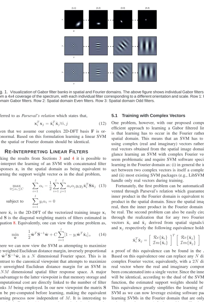
however, we have chosen to employ a Fourier representation in this paper due to its particularly useful ability to represent 2D convolution as a Hadamard product in the Fourier domain. A visualization of Gabor filters for 4 scales and 4 orienta-tions is presented in Figure 1. The top row shows the filters in the Fourier domain. In the spatial domain, the real part of the filter is even symmetric as shown in the second row. The third row shows the imaginary part of the spatial filter which is odd symmetric.
It has been demonstrated empirically in recent face iden-tity [6], [7] and expression [8], [9] recognition work, employ-ing linear classifiers, that improved classification performance can be attained if one employs an over-complete representa-tion zofx based on the concatenation of Gabor filter output responses,
z= [rT1, . . . ,rTM]T (3) whereM is the number of filter banks being employed.
3.1 Gabor Filters as a Weighted Inner Product It is elementary to prove that the inner product between any two vectors of concatenated linear filter responses is,
zTizj= M
X
m=1
rTm,irm,j (4)
where rm,i and rm,j are the mth filter vector responses for
the original raw appearance images xi and xj respectively.
According to Parseval’s relation [12] it can be shown that,
M X m=1 rTm,irm,j= M X m=1 ˆ rTm,iˆrm,j (5)
Based on Equation2we also know that in the Fourier domain,
M X m=1 ˆ rTm,iˆrm,j = M X m=1 ˆ xTidiag(ˆgm)Tdiag(ˆgm)ˆxj (6) = ˆxTiSˆxj (7) where, S= M X m=1 diag(ˆgm)Tdiag(ˆgm) (8)
and gˆm is themth vectorized 2D filter3 proving that
Equa-tion 4 is equivalent to Equation 7. It is interesting to note that in Equation 7 S can be pre-computed offline and the storage ofxˆi andxˆj remains static irrespective of the number
of filter banks M. Conversely, in Equation4 the storage and computation costs ofzi andzj are directly dependent on the
number of filter banks M.
3. Note that in Equation 6 we are taking advantage of the fact
that diag(ˆg)ˆx = ˆg·ˆxwhere diag()is an operator that transforms a N
dimensional vector into aN×N dimensional diagonal matrix. We should
also note that any transpose operator T on a complex vector or matrix in
this paper additionally takes the complex conjugate in a similar fashion to the
Hermitian adjoint [12].
4
L
INEARSVM
IN THEF
OURIERD
OMAIN Support vector machines (SVMs) have been demonstrated to be useful for many automatic classification tasks [14]. In particular, linear SVMs have proved popular in learning problems that have high-dimensional data (e.g., images, text, etc.) and large amounts of training examples [15]. Linear SVMs have a number of inherent advantages over kernel SVMs: (i) faster learning times, (ii) the ability to learn from larger datasets, (iii) low computation cost during evaluation (as the summation over support weights and vectors can be pre-computed) and most importantly, (iv) for some applications identitical if not superior performance to non-linear kernels (e.g., RBF, polynomial, tanh). Given a set of training example pairs (xi, yi) , i = 1, . . . , l, xi ∈ <N, yi ∈ {+1,−1}, alinear SVM attempts to find the solution to the following optimization problem, min w,ξi≥0 1 2w Tw+C l X i=1 ξi (9) subject to yiwTxi>1−ξi, i= 1. . . l
C is a penalty parameter, the biasb is accounted for inw←
[wT, b] by x ← [xT,1] and ξi are the “slack variables”
introduced to offset the effects of outliers in the final solution. This objective function can be equivalently expressed without slack variables as,
min w 1 2w Tw+C l X i=1 [1−yiwTxi]+ (10) where [z]+ = max(0, z) is referred to in literature [15] as the hinge error function. For brevity and conciseness we shall express the primal SVM objective function in this form from herein. Through solving this objective function we can learn a linear classifier that can obtain good generalization perfor-mance (i.e., maximizing the margin, which is proportional to minimizing wTw) while being tolerant to outliers (i.e., through the hinge error function).
Equation10is often referred to as solving the primal form of an SVM. One may instead solve the dual problem,
max 0≤αi≤C l X i=1 αi−1 2 l X i=1 l X j=1 αiαjyiyjxTi xj (11) subject to l X i=1 yiαi= 0
whereαiare the support weights. As pointed out by [11] it is
easy to see that the dual of Equation10is rotation invariant. For example if all xi were replaced by Axi, where A ∈ <N×N,ATA=I, then the solution to the dual remains the
same. Interestingly, one can view the application of a 2D-DFT as multiplication by a complex orthonormal basis xˆi = Fxi
whereFTF=I4. In signal processing this effect is commonly
4. It should be noted that in many practical formulations of a
2D-DFTFT
F = cI, where c is a constant. Typically, c = N where N is
the dimensionality of the feature space. In these circumstances it is trivial to show that an SVM should still be invariant to this scalar scaling given that
u v (1,1) ... x y ... x y ... (2,2) ... ... ... (3,3) ... ... ... (4,4)
Fig. 1. Visualization of Gabor filter banks in spatial and Fourier domains. The above figure shows individual Gabor filters stemming
from a 4x4 coverage of the spectrum, with each individual filter corresponding to a different orientation and scale. Row 1: Frequency domain Gabor filters. Row 2: Spatial domain Even filters. Row 3: Spatial domain Odd filters.
referred to as Parseval’s relation which states that,
xTi xj= ˆxTi ˆxj∀i, j (12)
given that we assume our complex 2D-DFT basis F is or-thonormal. Based on this formulation learning a linear SVM in the spatial or Fourier domain should be identical.
5
R
E-I
NTERPRETINGL
INEARF
ILTERSTaking the results from Sections 3 and 4 it is possible to re-interpret the learning of an SVM with concatenated filter responses zi in the spatial domain as being equivalent to
learning the support weight vectorα in the dual problem,
max 0≤αi≤C l X i=1 αi−1 2 l X i=1 l X j=1 αiαjyiyjxˆTiSxˆj (13) subject to l X i=1 yiαi= 0
where ˆxi is the 2D-DFT of the vectorized training image xi
andSis the diagonal weighting matrix of filters estimated in Equation8. Equivalently, one can view the prime problem as,
min ˆ w 1 2wˆ TS−1wˆ +C l X i=1 [1−yiwˆTxˆi]+ (14) where we can now view the SVM as attempting to maximize the weighted Euclidean distance margin, inversely proportional to wˆTS−1w, in aˆ N dimensional Fourier space. This is in contrast to the canonical viewpoint that attempts to maximize the unweighted Euclidean distance margin for an SVM in a N M dimensional spatial filter response space. A major disadvantage to the latter viewpoint is that memory storage and computational cost are directly linked to the number of filter banksM being employed. In our new viewpoint the matrixS can be pre-computed before learning, making the equivalent learning process now independent of M. It is interesting to note that in Equation14we are only manipulating the margin term, while the form of the hinge error term remains the same.
5.1 Training with Complex Vectors
One problem, however, with our proposed computationally efficient approach to learning a Gabor filtered linear SVM is that learning has to occur in the Fourier rather than the spatial domain. This means that an SVM has to be learnt using complex (real and imaginary) vectors rather than just real vectors obtained from the spatial image domain. At first glance learning an SVM with complex Fourier vectors may seem problematic and require SVM software specifically for learning in the Fourier domain as: (i) in general the inner prod-uct between two complex vectors is itself a complex number, and (ii) most existing SVM packages (e.g., LibSVM [16]) can handle only real vectors during training.
Fortunately, the first problem can be automatically circum-vented through Parseval’s relation which guarantees that the inner product in the Fourier domain is equivalent to the inner product in the spatial domain. Since the spatial images are all real, then the inner product in the Fourier domain must also be real. The second problem can also be easily circumvented through the realization that for any two Fourier complex vectors xˆi and xˆj derived from spatial signals/images xi
andxj respectively the following equivalence holds,
ˆ xTixˆj = Re{xˆi} Im{ˆxi} T Re{xˆj} Im{ˆxj} (15) a proof of this equivalence can be found in the Appendix. Based on this equivalence one can replace anyN dimensional complex Fourier vector, equivalently, with a2N dimensional real vector where the real and imaginary components have been concatenated into a single vector. Since the inner products will be identical, according to the dual of the SVM objective function, the estimated support weights should be identical. This equivalence greatly simplifies the learning of the linear SVM as we can now leverage existing software packages for learning SVMs in the Fourier domain that are only designed to handle real vectors. A further problem still exists, however, with respect to the application of our approach to traditional
0 25 50 75 100 0 25 50 75 100 AU :1 Raw pixels Best Gabor:8x8 0 25 50 75 100 0 25 50 75 100 AU :2 Raw pixels Best Gabor:4x4 0 25 50 75 100 0 25 50 75 100 AU :4 Raw pixels Best Gabor:64x64 0 25 50 75 100 0 25 50 75 100 AU :5 Raw pixels Best Gabor:4x4 0 25 50 75 100 0 25 50 75 100 AU :6 Raw pixels Best Gabor:8x8 0 25 50 75 100 0 25 50 75 100 AU :7 Raw pixels Best Gabor:4x4 0 25 50 75 100 0 25 50 75 100 AU :9 Raw pixels Best Gabor:4x4 0 25 50 75 100 0 25 50 75 100 AU :12 Raw pixels Best Gabor:8x8 0 25 50 75 100 0 25 50 75 100 AU :15 Raw pixels Best Gabor:8x8 0 25 50 75 100 0 25 50 75 100 AU :17 Raw pixels Best Gabor:32x32 0 25 50 75 100 0 25 50 75 100 AU :20 Raw pixels Best Gabor:8x8 0 25 50 75 100 0 25 50 75 100 AU :23 Raw pixels Best Gabor:4x4 0 25 50 75 100 0 25 50 75 100 AU :24 Raw pixels Best Gabor:32x32 0 25 50 75 100 0 25 50 75 100 AU :25 Raw pixels Best Gabor:32x32 0 25 50 75 100 0 25 50 75 100
False acceptance rate, %
False rejection rate, %
AU :27 Raw pixels Best Gabor:4x4
Fig. 2. DET curves for different AUs. DET corresponding to raw pixles along side the DET for the number of Gabor filters that
gave the best performance. For different AUs, different numbers of Gabor filters gave small changes in performance. The variation in performance for varying numbers of Gabor filters, however, was small compared to the difference in performance between using and not using (i.e., raw) the filters. Empirical evidence of this effect can be seen in Figure3.
SVM learning packages as they are traditionally maximizing a Euclidean distance margin, as described in Equation10, rather than our reinterpreted weighted Euclidean distance margin described in Equation 14. This problem can be remedied in practice by multiplying each Fourier examplexˆi in the train
set by√Sbefore learning the support vector weightsαin the dual form.
5.2 Testing without Filtering
The outcome of the SVM training step is the weight vectorwˆ
(See Equation 14) and a bias b. The weight vector wˆ can be computed from the dual form (See Equation 13) as follows:
ˆ w=S l X i=1 αiyixˆi (16)
Since the SVM is trained in the Fourier domain, we would need to compute the Fourier transform of a test image, if we want to use wˆ during testing. However, we can again exploit Parseval’s relation to now improve computational efficiency in testing. By virtue of Parseval’s relation we know,
ˆ
wTxˆ=wTx (17) wherewis the inverse Fourier transform of the weight vector
ˆ
w, and x represents the test image. We may thus use the following decision rule directly on the input imagex,
wTx true
≷ false
b (18)
Thus at testing time we do not need to compute the Fourier transform of an incoming test image, and operate directly in the image domain.
6
E
VALUATIONThough the techniques presented in Section5can be applied to an array of computer vision problems, we present an applica-tion of our technique to the task of expression recogniapplica-tion. Specifically, we conducted experiments for detecting facial action units (AUs). AUs are the smallest visibly discriminable changes in facial expression. Within the FACS (Facial Action Coding System) [17], [18], 44 distinctive AUs have been defined. The experiments were conducted on the Cohn-Kanade FACS-Coded Facial Expression Database [13]. This database consists of approximately 500 sequences of 100 subjects. Each video frame is FACS coded indicating the presence or absence of each of the AUs. The faces were first coarsely registered so that the eye coordinates align, the line joining the eyes is horizontal, and the distance between the eyes is nominal. The face area was cropped to give a70×100image.
Typically, when an AU is annotated there may be a time stamp noted for its onset (i.e., start), offset (stop) and/or peak (maximum intensity). For the Cohn-Kanade database, time stamps were provided for onset and peak AU intensity of each image sequence. Onset time stamps were assumed to be representative of a local AU 0 (i.e. neutral expression). We make use of AU 0 to achieve subject normalization in our experiments. In previous work [19], [20], [21] it has been demonstrated that some form of subject normalization is ben-eficial in terms of recognition performance. The employment
Raw8 4x4 8x8 16x16 32x32 64x64 128x128 10 12 14 16 18 20 Avg. EER (%)
Gabor filter bank size
Fig. 3. Overall performance across all AUs tested. The plot
shows the average equal error rate as a function of Gabor filter bank size.
of delta features are a particularly useful method for subject normalization. The delta features are obtained by subtracting the neutral time stamp of the same subject from the peak time stamp.
In this paper we present AU detection results for 15 AUs. For every AU we learn a “one versus all” binary SVM clas-sifier on Gabor representations derived from the application of a bank of Gabor filters of varying number of spatial frequencies and orientations, using the formulation detailed in Section 5. Specifically, we trained classifiers employing Gabor filter banks ranging from 4×4 to128×128. A bank of 128×128 Gabor filters corresponds to an ensemble of filters describing 128 individual spatial frequencies and 128
orientations, which for an image size of70×100, amounts to a feature dimensionality of128×128×70×100≈1.15×10⁸, if one chooses to use conventional methods. To allow maximum usage of the training data, we employed a leave-one-subject-out cross validation. As a baseline, we learnt classifiers on raw pixels as well.
The performance of a detection system is usually character-ized by a Detection Error Tradeoff (DET) curve, which is a plot of the relation between the false acceptance rate and the false rejection rate. For a particular AU, the false acceptance rate represents the proportion of images for which an AU is absent in the ground truth, but the classifier still detects it. The false rejection rate represents the rejection of true presence of an AU. Often, a detection system is gauged in terms of the Equal Error Rate (EER). The EER is determined by finding the point on the DET curve at which the two errors, the false acceptance rate, and the false rejection rate, are equal. 6.1 Experiments with Filter Bank Size
In Figure2we present for each AU the DET curve correspond-ing to raw pixels along side the DET curve for the number of Gabor filters that gave the best performance (in terms of EER). For all AUs the use of Gabor features, as a pre-processing step, outperforms the performance on raw pixels. This result is consistent with current leading literature in expression recognition [8], [9]. Unlike these previous studies, however, no approximation to the full Gabor filtered representation is made. Moreover, we are able to analyze finely resolved Gabor filters, a hitherto untestable task. We present the overall performance across all the action units by the average EER plot shown in Figure 3.
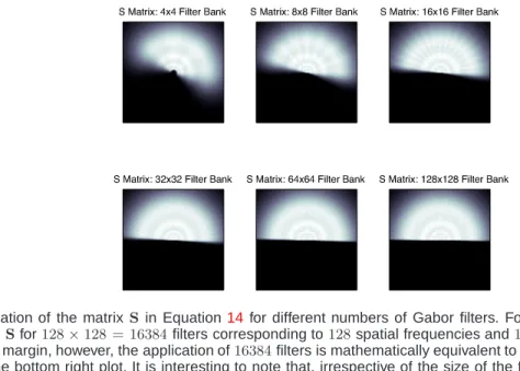
For different AUs different filter bank sizes gave varying performance. The variation in performance for varying num-bers of Gabor filters, however, was small compared to the difference in performance between using and not using (i.e., raw) the filters. This empirical result can be seen in Figure3 where there is virtually no change in average EER after the application of4×4banks of Gabor filters. This result is consis-tent with our new view of Gabor filters as simply a weighting matrixS in the Fourier domain, which is independent of the number of filters being employed. Visualizations in the 2D Fourier domain of the diagonal elements of S can be seen in Figure 4 for different filter bank sizes. It is interesting to note that irrespective of the filter bank size the visualization ofS in the Fourier domain remains similar, thus reinforcing the empirical results seen in Figure3.
6.2 Experiments with Downsampling and Normalization
We now present in Figure 5 a comparison between our method with the approximation method advocated by Liu et al. [7]. In order to circumvent the problem of high dimensionality, Liu first downsample the individual Gabor response by a factor of ρ. They then normalize the downsampled responses such that it has zero mean and unit variance. We should emphasize that all raw pixel cropped face images in our experiments had zero mean and unit variance. We present a comparison for 8×8 Gabor filters, and set ρ = 64 as done in [7]. Without normalization, we get an average EER of 13.6% on donwnsampled Gabor responses. With normalization, we im-prove our result to an average EER of12.35%. In contrast our method, without any normalization, using8×8 Gabor filters gives a substantially superior average EER of 9.56%. This demonstrates that downsampling the Gabor responses indeed discards, unnecessarily, useful information for classification. With our technique, we are able to leverage on all the infor-mation available in the Gabor responses, without incurring the additional computational and memory costs associated with the canonical approach.
7
D
ISCUSSIONThe results in Figures 3 and 4 are of particular interest when one is rationalizing the employment of filter banks, like Gabor and others, as a pre-processing step before classification of visual phenomena using a linear SVM. Often, this type of work has been muddied by questions like: “How many filter banks should we choose?”, “How should the filters be distributed in the frequency spectrum?”, “What class of filter wavelets should we employ (e.g., Gabor, Log Gabor, Harr, etc.)?”. Attempts to answer these questions have often been based previously on heuristics or qualitative biological motivations. As we have discussed throughout this paper, most of these questions can be largely circumvented if one views the application of these filters as a manipulation of the margin, through the weighting matrixS, within a linear SVM. A more interesting question should perhaps be now: “What is the best S to use for my application?” and ignore the question of filtering completely. This answer on how to select/learnS is a topic for future research.
!" #$%#$% !" && !" %% !" #&#& !" '$'$ !"
Fig. 4. Visualization of the matrixS in Equation14 for different numbers of Gabor filters. For instance, the bottom right plot
shows the matrixSfor128×128 = 16384filters corresponding to128spatial frequencies and128orientations. In the context of maximizing SVM margin, however, the application of16384filters is mathematically equivalent to a single filter in Fourier space as represented in the bottom right plot. It is interesting to note that, irrespective of the size of the filter banks the visualization ofS remains approximately the same.
We should also note, that in many circumstances in literature [7] the response from each filter has had a non-linear operation applied which further improves performance. A good example of this can be seen in the power normalization filter response step of Liu et al. [7]. In our work we demonstrated that the ability to preserve the full resolution response outweighs the benefit obtained from Liu’s method for the task of expression recognition. A topic of additional future work, however, shall be on how to introduce such non-linear operations while keeping the computational and memory advantages of our proposed technique.
8
C
ONCLUSIONSIn this paper we have presented a reinterpretation of the application of Gabor filters, as a pre-processing step, to a linear SVM in terms of a manipulation of the margin that is being maximized. A major advantage of this reinterpretation is that it circumvents the large memory and computational requirements if one was to learn a linear SVM in the tra-ditional manner. Conventionally, a linear SVM is learnt by attempting to maximize the canonical Euclidean SVM margin using Gabor preprocessed images. In our new formulation, we demonstrated the same linear SVM can be learnt by maximizing a weighted Euclidean distance margin for the unfiltered images in the Fourier domain, eliminating the need to compute Gabor preprocessed images. Additionally, we demonstrated that through this reinterpretation the computa-tional and memory requirements were invariant to the size of the filter banks being employed, allowing for the exploration of hitherto unimaginable filter bank configurations. Moreover, we made use of Parseval’s relation to circumvent the need for computing the Fourier transform of an input image during evaluation, thus allowing for the direct application of the linear SVM to the raw pixels of a test image.
Our approach is able to use conventional SVM packages for learning the SVM even though it relies on complex training
0 2 4 6 8 10 12 14 Our method Avg. EER (%)
Gabor downsampling Gabor downsampling with normalization, [7]
Fig. 5. Comparison between our approach and downsampling
of Gabor responses [7]. The results show that discarding the information in Gabor responses by downsampling them results in a performance loss (EER: 12.35%). Our method gives the lowest EER (9.56%), as we are making use of all the available information without additional computational burden
vectors as a result of the application of the 2D-DFT. We have additionally demonstrated improved performance for the challenging task of action unit recognition. We have shown that the downsampling of Gabor responses as done in [7] results in a performance loss, compared to our approach, as it discards useful information. With our computationally efficient approach we are able to make full use of the available information giving improved performance.
A
PPENDIXC
OMPLEX TOR
EALI
NNERP
RODUCTSIn this section we prove the result given in Equation 15. Consider any twoN dimensional complex vectors,
xi= a0+jb0 a1+jb1 .. . aN−1+jbN−1 ,xk = c0+jd0 c1+jd1 .. . cN−1+jdN−1
we use the notationxto denote a complex vector as opposed to xˆ which denotes the complex Fourier representation of a real signal x. The inner product between xi and xk can be
written as, xTixk = [a0−jb0· · ·aN−1−jbN−1] c0+jd0 . .. cN−1+jdN−1 = N−1 X n=0 (ancn+bndn) +j N−1 X n=0 (andn−bncn)
So in general, we see that the inner product of two complex vectors is in itself a complex number. Fortunately, however, complex Fourier vectors xˆ have additional symmetry and structure that can be leveraged. For the case of a 1D DFT ofxwhere the dimensionality N is odd we know,
ˆ
x(n) =conj{xˆ(N−n)}, n= 1, . . . ,(N−1)/2 (19) where xˆ(0), referring to the DC component, is always real. Therefore obtaining the inner product between any two oddN
length 1D Fourier complex vectorsxˆi andxˆk becomes,
ˆ xTixˆk = a0+ (N−1)/2 X n=1 (an−jbn)(cn+jdn) (20) + (N−1)/2 X n=1 (an+jbn)(cn−jdn) = a0+ (N−1)/2 X n=1 2(ancn+bndn) (21) demonstrating, as Parseval’s relation implies, that xˆTixˆk will
always be a real scalar. For the case where N is even this equivalence still holds, but aN/2 is additionally added which is also guaranteed of being real. Further, based on Equation20 it is trivial to show that,
ˆ
xTi ˆxk=Re{xˆi}TRe{xˆk}+Im{xˆi}TIm{ˆxk} (22)
where this equivalence can be shown to hold not only for 1D DFTs, but DFTs of 2D and higher by leveraging a similar symmetry as in the 1D case. As a consequence of Equation22 it is possible to employ learning packages that are designed to handle only real vectors and their inner products by expressing any N dimensional complex Fourier vector xˆ as the 2N
dimensional real vector,
Re{xˆ}
Im{ˆx}
as the inner products will always be equivalent. Further, it is possible to show through intelligent indexing of the complex
Fourier vector xˆ that a real vector can be obtained that is only N, rather than 2N dimensional which can lead to additional memory and computational savings. The form of this indexing procedure, however, for the case of an 2D-DFT is outside the scope of this paper.
R
EFERENCES[1] D. Gabor, “Theory of communication,” Journal of the Institution of
Electrical Engineers (London), vol. 93, no. III, pp. 429–457, 1946.1,2
[2] J. G. Daugman, “Two-dimensional spectral analysis of cortical receptive
field profiles,” Vision Research, vol. 20, no. 10, pp. 847–856, 1980. 1,
2
[3] J. Daugman, “Uncertainty relation for resolution in space, spatial
fre-quency, and orientation optimized by two-dimensional cortical filters,”
Journal of the Optical Society of America, vol. 2, no. 7, pp. 1160–1169,
1985. 1,2
[4] J. G. Daugman, “Complete discrete 2-D Gabor transforms by neural
networks for image analysis and compression,” IEEE Trans. Pattern
Analysis and Machine Intelligence, vol. 36, pp. 1169–1179, July 1988. 1,2
[5] D. J. Field, “Relations between the statistics of natural images and the
response properties of cortical cells,” Journal of the Optical Society of
America A, vol. 4, no. 12, pp. 2379–2393, 1987. 1,2
[6] C. Wiskott, J. M. Fellous, N. Kr¨uger, and C. von der Malsburg, “Face
recognition by elastic bunch graph matching,” IEEE Trans. Pattern
Analysis and Machine Intelligence, vol. 19, no. 7, pp. 775–779, July
1997. 1,2,3
[7] C. Liu and H. Wechsler, “Gabor feature based classification using the
enhanced Fisher linear discriminant model for face recognition,” IEEE
Trans. Image Processing, vol. 11, no. 4, pp. 467–476, 2002. 1,2,3,6,
7
[8] M. S. Bartlett, G. Littlewort, M. Frank, C. Lainscesk, I. Fasel, and
J. Movellan, “Recognizing facial expression: Machine learning and application to spontaneousbehavior,” IEEE Conference on Computer
Vision and Pattern Recogntion, vol. 2, pp. 568–573, June 2005.1,2,3,
6
[9] M. Bartlett, G. Littlewort, C. Lainscsek, I. Fasel, M. Frank, and
J. Movellan, “Fully automatic facial action recognition in spontaneous behavior,” 7th International Conference on Automatic Face and Gesture
Recognition, 2006. 1,2,3,6
[10] Z. Li, D. Lin, and X. Tang, “Nonparametric discriminant analysis for face recognition,” IEEE Trans. Pattern Analysis and Machine
Intelli-gence, vol. 31, no. 4, pp. 755–761, April 2009. 1,2
[11] P. K. Shivaswamy and T. Jebara, “Relative margin machines,” in Neural
Information Processing Systems 21 (NIPS), 2008. 1,3
[12] A. V. Oppenheim and A. S. Willsky, Signals & Systems, 2nd ed.
Prentice Hall, 1996. 1,2,3
[13] T. Kanade, J. F. Cohn, and Y. Tian, “Comprehensive database for facial expression analysis,” IEEE International Conference on Automatic Face
and Gesture Recognition, pp. 46–53, 2000. 1,5
[14] B. E. Boser, I. Guyon, and V. Vapnik, “A training algorithm for optimal margin classifiers,” in 5th Annual ACM Workshop on Computational
Learning Theory (COLT), 1992. 3
[15] R.-E. Fan, K.-W. Chang, C.-J. Hsieh, X.-R. Wang, and C.-J. Lin, “LIBLINEAR: A library for large linear classification,” Journal of
Machine Learning Research, vol. 9, pp. 1871–1874, 2008. 3
[16] C.-C. Chang and C.-J. Lin, LIBSVM: a library for
support vector machines, 2001, software available at
http://www.csie.ntu.edu.tw/∼cjlin/libsvm. 4
[17] P. Ekman and W. V. Friesen, Facial action coding system. Palo Alto,
CA: Consulting Psychologists Press, 1978. 5
[18] P. Ekman, W. V. Friesen, and J. Hager, Facial action coding system:
Research Nexus. Salt Lake City, UT: Network Research Information,
2002. 5
[19] S. Lucey, A. B. Ashraf, and J. Cohn, “Investigating spontaneous facial action recognition through aam representations of the face,” in Face
Recognition Book, K. Kurihara, Ed. Mammendorf, Germany: Pro
Literatur Verlag, April 2007. 5
[20] S. Lucey and T. Chen, “Learning patch dependencies for improved pose mismatched face verification,” in IEEE International Conference
on Computer Vision and Pattern Recognition (CVPR), June 2006. 5
[21] J. Cohn, A. Zlochower, J.-J. J. Lien, and T. Kanade, Automated face
analysis by feature point tracking has high concurrent validity with manual FACS coding, vol. 36, pp. 35 – 43, 1999. 5