Journal of Approximation Theory 163 (2011) 1834–1853
www.elsevier.com/locate/jat
Full length article
A new linear spectral transformation associated with
derivatives of Dirac linear functionals
Kenier Castillo
a, Luis E. Garza
b,∗, Francisco Marcell´an
a aDepartamento de Matem´aticas, Escuela Polit´ecnica Superior, Universidad Carlos III, Legan´es, Madrid, SpainbFacultad de Ciencias, Universidad de Colima, Bernal D´ıaz del Castillo No.340, Colima, Colima, Mexico
Received 30 November 2010; received in revised form 20 May 2011; accepted 10 August 2011 Available online 17 August 2011
Communicated by Andrei Martinez-Finkelshtein
Abstract
In this contribution, we analyze the regularity conditions of a perturbation on a quasi-definite linear functional by the addition of Dirac delta functionals supported on N points of the unit circle or on its complement. We also deal with a new example of linear spectral transformation. We introduce a perturbation of a quasi-definite linear functional by the addition of the first derivative of the Dirac linear functional when its support is a point on the unit circle or two points symmetric with respect to the unit circle. Necessary and sufficient conditions for the quasi-definiteness of the new linear functional are obtained. Outer relative asymptotics for the new sequence of monic orthogonal polynomials in terms of the original ones are obtained. Finally, we prove that this linear spectral transform can be decomposed as an iteration of Christoffel and Geronimus linear transformations.
c
⃝2011 Elsevier Inc. All rights reserved.
Keywords:Orthogonal polynomials on the unit circle; Hermitian linear functionals; Quasi-definite linear functionals; Verblunsky parameters; Carath´eodory functions; Outer relative asymptotics
1. Introduction
Let us consider the linear space of Laurent polynomials with complex coefficients Λ =
span{zk}k∈Z as well as the linear subspace P of polynomials with complex coefficients. Let
∗Corresponding author.
E-mail addresses:[email protected](K. Castillo),[email protected](L.E. Garza), [email protected](F. Marcell´an).
0021-9045/$ - see front matter c⃝2011 Elsevier Inc. All rights reserved. doi:10.1016/j.jat.2011.08.003
Lbe a linear functional inΛsuch that cn=L,zn=L,z−n= ¯c−n,
i.e.Lis a Hermitian linear functional. InPwe can associate withLa bilinear functional such that
⟨p(z),q(z)⟩L= L,p(z)q(z−1). The set of complex numbers{ck}k∈Zare called themoments
associated withL, and the Gram matrix associated withLis the Toeplitz matrix
T= c0 c1 · · · cn · · · c−1 c0 · · · cn−1 · · · ... ... ... ... c−n c−n+1 · · · c0 · · · ... ... ... ... . (1)
Let us denote byTn, the(n+1)×(n+1)principal leading submatrix ofT. If det(Tn)̸=0 for
everyn ⩾0, thenLis said to be a quasi-definite (or regular) linear functional. In such a case, there exists a family of monic polynomials{Φn}n⩾0satisfying
L,Φn(z)Φm(z−1)
=knδn,m, n,m⩾0,
wherekn = ‖Φn(z)‖2 ̸= 0,n ⩾ 0.{Φn}n⩾0is said to be the sequence of monic orthogonal
polynomials (MOPS) with respect toL. Furthermore, we havekn=det(Tn)/det(Tn−1),n⩾1,
with the conventionk0=c0.
If det(Tn) >0 for everyn ⩾0, thenLis said to be a positive definite linear functional, and
the integral representation holds (see [8,11])
⟨L,p(z)⟩ =
∫
T
p(z)dσ (z),
where p(z)∈ Pand dσ is a nontrivial positive measure supported onT, which can be
decom-posed into dσ = σ′dθ
2π +dσs, i.e. an absolutely continuous part with respect to the Lebesgue
measure and a singular part. Unless otherwise noted, throughout the manuscript we will consider quasi-definite linear functionals.
The properties of {Φn}n⩾0 have been extensively studied (see [8,7,17,18], among others).
They satisfy Φn+1(z)=zΦn(z)+Φn+1(0)Φn∗(z), n⩾0, (2) Φn+1(z)= 1− |Φn+1(0)|2 zΦn(z)+Φn+1(0)Φn∗+1(z), n ⩾0, (3)
the so-called forward and backward recurrence relations, where Φn∗(z) = znΦ¯n(z−1)is the
reversed polynomial and the complex numbers{Φn(0)}n⩾1are known as Verblunsky coefficients
(they are also called either Schur or reflection parameters). It is important to notice that|Φn(0)| ̸=
1,n ⩾ 1 (for positive definite linear functionals, we have|Φn(0)| < 1,n ⩾1). Furthermore,
there is a one to one correspondence between a linear functional (or its corresponding measure), its sequence of moments, and its family of Verblunsky coefficients [17]. Then-th reproducing kernel is given by Kn(z,y)= n − m=0 Φm(z)Φm(y) km = Φ ∗ n+1(y)Φ ∗ n+1(z)−Φn+1(y)Φn+1(z) kn+1(1− ¯yz) , (4)
where the last identity holds ifzy¯ ̸= 1. It is known in the literature as Christoffel–Darboux formula. We denote byKn(j,k)(z,y)the j-th (resp.k-th) derivative ofKn(z,y)with respect to the
variablez(resp.y).
In terms of the moments, we can define the function F(z)=c0+2
∞
−
k=1
c−kzk. (5)
IfLis positive definite, F is an analytic function with positive real part inD. Moreover, it has
the integral representation F(z)=
∫
T
w+z w−zdσ (w),
whereσis the measure associated withL.F(z)is said to be the Carath´eodory function associated withL. For quasi-definite linear functionals, we will defineF(z)as(5).
Given a linear functionalL, the following perturbations have been studied in the last years (see [5,6,9,10,13–15] among others)
1. ⟨p(z),q(z)⟩L C = ⟨(z−α)p(z), (z−α)q(z)⟩L,α∈C. 2. ⟨p(z),q(z)⟩L G = p(z) z−α, q(z) z−α L+mp(α)q(α¯ −1)+ ¯mp(α¯−1)q(α),α∈ C,|α| ̸=1,m∈C. 3. ⟨p(z),q(z)⟩L U = ⟨p(z),q(z)⟩L+mp(α)q(α¯ −1)+ ¯mp(α¯−1)q(α),m∈ C,|α|>1.
The corresponding family of orthogonal polynomials, the Carath´eodory function, and the associated Hessenberg matrix (the matrix representation of the multiplication operator in the canonical basis of the linear space of polynomials), as well as necessary and sufficient conditions for the regularity of the perturbed functionals have been deeply analyzed in the literature.
The above perturbations are called, respectively, Christoffel (FC(α)), Geronimus (FG(α,m)),
and Uvarov (FU(α,m)). They are related by
(i) FC(α)◦FG(α,m)=I(Identity transformation),
(ii) FG◦FC(α)=FU(α,m).
In particular, we will focus our attention in the Uvarov transformation. The simplest of this kind of transformations is defined by
⟨p(z),q(z)⟩L
U = ⟨p(z),q(z)⟩L+mp(α)q(α), m∈R,|α| =1, (6) i.e. the addition of a real mass on a point located on the unit circle, and it was analyzed in [5], where the authors obtained necessary and sufficient conditions for the regularity of LU, the
relation between the corresponding families of orthogonal polynomials, Carath´eodory functions, Hessenberg matrices, and Verblunsky coefficients. Later on, a generalization of this problem for positive definite linear functionals was studied in [20], where the author studied, among other properties, the asymptotic behavior of the Verblunsky parameters whenNreal masses are added on the unit circle.
If the mass points are located outside the unit circle, then the perturbation becomes
⟨p(z),q(z)⟩L
U = ⟨p(z),q(z)⟩L+mp(α)q(α¯
−1)+ ¯mp(α¯−1)q(α),
m∈C,|α|>1, (7)
where complex conjugates are considered in order to preserve the Hermitian character ofLU.
It is not so difficult to show that, in terms of the moments, perturbations(6)and(7)can be expressed, respectively, as ˜ ck=ck+mαk, k∈Z, (8) ˜ ck=ck+mαk+ ¯mα¯−k, k∈Z. (9)
Furthermore, in both cases the corresponding Carath´eodory functions are related by
F(z)= A(z)F(z)+B(z)
D(z) , (10)
where A,B, and D are polynomials whose coefficients depend on mand α (see [14]). The complex function Fdefined by (10) is said to be a linear spectral transformation of F(z).
In the case of measures supported on the real line, linear spectral transformations have been analyzed in [21], where the author proves that any transformation of the form(10)to a Stieltjes function can be expressed in terms of Christoffel and Geronimus transformations. Notice that in the cases described above, the class of linear transformations is quite rich and new examples appear. Indeed, in [3] a perturbation involving the addition of masses was studied. There, the authors considered the addition of a Lebesgue measure to a linear functional, i.e.
⟨p(z),q(z)⟩L0 := ⟨p(z),q(z)⟩L+m
∫
T
p(z)q(z) dz
2πiz, m∈R. (11) Notice that only the first moment is perturbed, and thusc˜0=c0+m,c˜k =ck,k ∈Z {0}. In
other words, this is equivalent to perturb the main diagonal of the corresponding Toeplitz matrix by
T=T+mI, (12)
whereI is the semi-infinite identity matrix. A particular case form = 1 was studied on [1] and the regularity conditions for(11), as well as an expression for the corresponding family of orthogonal polynomials, were obtained in [3].
The generalization of the previous perturbation to affect any subdiagonal of the Toeplitz matrix is defined by ⟨p(z),q(z)⟩L j := ⟨p(z),q(z)⟩L+m zjp(z),q(z) Lθ + ¯m p(z),zjq(z) Lθ, (13) where m ∈ C, andLθ is the linear functional associated with the Lebesgue measure. The corresponding analysis was developed in [4]. In terms of the Toeplitz matrix, we have
T=T+ 0 · · · m 0 · · · ... 0 · · · m · · · ¯ m ... ... ... ... 0 m¯ · · · 0 · · · ... ... ... ... ... ,
i.e., only the j-th sub-diagonal and upper-diagonal are perturbed.
It is not difficult to see that perturbations (11)and(13) can be expressed, in terms of the corresponding Carath´eodory functions, as
F0(z)=F(z)+m,
Fj(z)=F(z)+2mzj,
so they are also linear spectral transformations in the sense of(10).
The aim of our contribution is to introduce two new examples of linear spectral transformations associated with the first derivative of the Dirac linear functional. The first one appears when the support of the Dirac linear functional is a point in the unit circle. The second one corresponds to a Dirac linear functional supported on two symmetric points with respect to the unit circle. The structure of the manuscript is as follows.
In Section2, an Uvarov perturbation of a quasi-definite linear functional by a Dirac linear functional supported onN points located either on the unit circleTor on its complement is
in-troduced. Necessary and sufficient conditions for the regularity of the perturbed linear functional are deduced. In Section3, we deal with the addition of a linear functional that is the derivative of a Dirac linear functional supported either on a point located on the unit circleTor on two
points symmetric with respect to the unit circle. Both situations can be considered as limit cases of the previous one but the difficulties to deal with them yield a different approach. We prove the regularity of the perturbed linear functionals as well as the outer relative asymptotics of the new MOPS in terms of the initial MOPS. In Section4, we prove that they are linear spectral trans-formations using the relation between the corresponding Carath´eodory functions. Furthermore, we obtain their representation in terms of Christoffel and Geronimus transformations. Finally, in Section5, some illustrative examples are presented.
2. Uvarov perturbation withNmasses
Let us start our analysis with a generalization of the perturbation(6). Consider a quasi-definite functionalL and let LΥ be the linear functional such that its associated bilinear functional
satisfies ⟨p,q⟩L Υ = ⟨p,q⟩L+ N − i=1 mip(αi)q(αi), (14)
wheremi ∈R\ {0}and|αi| =1 fori =1, . . . ,N. Using an analogue method to the one used
in [5], we can show the following proposition.
Proposition 1.The following statements are equivalent. (i) LΥ is a quasi-definite linear functional.
(ii) The matrixRNn−1+M−N1is non singular, and kn+ [8nN(α)] t(RN n−1+M −1 N ) −18N n(α)̸=0, n⩾1. (15)
Moreover, the sequence of monic polynomials orthogonal with respect toLΥ is given by
Υn(z)=Φn(z)−KnN−1(z)(R N n−1+M −1 N ) −18N n(α), n⩾1, (16) withKnN−1(z)= [Kn−1(z, α1),Kn−1(z, α2), . . . ,Kn−1(z, αN)],MN =diag{m1,m2, . . . ,mN}, 8N n(α)= [Φn(α1),Φn(α2), . . . ,Φn(αN)]t and RnN−1= Kn−1(α1, α1) Kn−1(α1, α2) · · · Kn−1(α1, αN) Kn−1(α2, α1) Kn−1(α2, α2) · · · Kn−1(α2, αN) ... ... ... ... Kn−1(αN, α1) Kn−1(αN, α2) · · · Kn−1(αN, αN) .
Proof. First, assume that LΥ is a quasi-definite linear functional and denote by {Υn}n⩾0 its
corresponding sequence of monic orthogonal polynomials. Thus, forn ⩾1,
Υn(z)=Φn(z)+ n−1 − k=0 λn,kΦk(z), whereλn,k = − N ∑ i=1 miΥn(αi)Φk(αi) kk , n≥1. Then, we have Υn(z)=Φn(z)− N − i=1 miΥn(αi)Kn−1(z, αi). (17)
In particular, for j = 1, . . . ,N, we have the following system of N linear equations and N unknownsΥn(αj), j=1,2, . . . ,N Υn(αj)=Φn(αj)− N − i=1 miΥn(αi)Kn−1(αj, αi). Therefore, 1+m1Kn−1(α1, α1) m2Kn−1(α1, α2) · · · mNKn−1(α1, αN) m1Kn−1(α2, α1) 1+m2Kn−1(α2, α2) · · · mNKn−1(α2, αN) ... ... ... ... m1Kn−1(αN, α1) m2Kn−1(αN, α2) · · · 1+mNKn−1(αN, αN) ϒN n(α) =8nN(α),
whereϒnN(α) = [Υn(α1),Υn(α2), . . . ,Υn(αN)]. In other words,(RnN−1MN +IN)ϒ N n(α) = 8N
n(α). SinceLΥ is assumed to be quasi-definite, the matrix(RnN−1MN +IN)is non singular
and, therefore,(16)follows from(17).
On other hand, assume (ii) holds. For 0≤k≤n−1, we have
⟨Υn(z),Φk(z)⟩LΥ = Φn(z)− N − i=1 miΥn(αi)Kn−1(z, αi),Φk(z) + N − i=1 miΥn(αi)Φk(αi) = − N − i=1 miΥn(αi)⟨Kn−1(z, αi),Φk(z)⟩ + N − i=1 miΥn(αi)Φk(αi)=0,
using the reproducing kernel property in the last expression. Furthermore,
⟨Υn(z),Φn(z)⟩LΥ =kn+ N − i=1 miΥn(αi)Φn(αi) =kn+ [8 N n(α)]tMNϒNn =kn+ [8nN(α)] t(RN n−1+M −1 N ) −18N n(α)̸=0,
which proves that{Υn}n⩾0 defined by(16)is the sequence of monic polynomials orthogonal
Remark 2. Notice that forN =1, the regularity condition forLΥbecomes 1+m1Kn−1(α1, α1)
̸=0,n ≥0, as shown in [5].
Evaluating(16)inz=0, we get the following corollary. Corollary 3. For n⩾1, Υn(0)=Φn(0)−KNn−1(0)(R N n +M −1 N ) −18N n(α). (18)
The previous expression allows us to obtain the Verblunsky coefficients associated with the perturbed polynomials directly, provided that the original Verblunsky coefficients are known.
Proposition 4.For z∈D, the Carath´eodory function associated withLΥis
FΥ(z)=F(z)+ N − i=1 mi α i+z αi−z . Proof. Denotingc−˜ k = ⟨LΥ,z−k⟩, we have
FΥ(z)= ˜c0+2 ∞ − k=1 ˜ c−kzk =c0+2 ∞ − k=1 c−kzk+ N − i=1 mi+2 ∞ − k=1 N − i=1 miα¯ikz k = F(z)+ N − i=1 mi α i+z αi−z , i.e.,FΥ(z)has simple poles atz=αi.
The next step is to consider a perturbation of the form(7), generalizing forN masses, i.e. to consider the linear functionalLΩ such that its corresponding bilinear functional satisfies
⟨p,q⟩L Ω = ⟨p,q⟩L+ N − i=1 (mip(αi)q(α−i 1)+mip(α¯−i 1)q(αi)), (19)
where|αi| ̸=0,1 andmi ∈C{0}, 1⩽i ⩽ N. By analogy with the previous case, we have
the following result.
Proposition 5.The following statements are equivalent. (i) LΩ is a quasi-definite linear functional.
(ii) The matrixR2Nn−1+M−2N1is non singular, and kn+ [8
2N
n (α)]tM2N2Nn (α)̸=0, n ⩾1. (20)
Moreover, the corresponding sequence of monic polynomials orthogonal with respect toLΩ is given by Ωn(z)=Φn(z)−K2Nn−1(z)(R 2N n−1+M −1 2N) −182N n (α), n⩾1, (21)
with K2Nn−1= [Kn−1(z, α1), . . . ,Kn−1(z, αN),Kn−1(z, α−11), . . . ,Kn−1(z, α−N1)], M2N =diag{m1, . . . ,mN,m1, . . . ,mN}, 82N n (α)= [Φn(α1), . . . ,Φn(αN),Φn(α−11), . . . ,Φn(α−N1)]t, R2Nn−1= Rn−1(α1,N, α1,N) Rn−1(α1,N,α¯−1,1N) Rn−1(α¯1−,1N, α1,N) Rn−1(α¯−1,1N,α¯−1,1N) , and Rn−1(α1,N, α1,N)= Kn−1(α1, α1) · · · Kn−1(α1, αN) ... ... ... Kn−1(αN, α1) · · · Kn−1(αN, αN) .
Proceeding as in the proof orProposition 4, we obtain the following proposition. Proposition 6. For z∈D, FΩ(z)=F(z)+ N − i=1 miαi +z αi−z + ¯mi ¯ α−1 i +z ¯ α−1 i −z . i.e.,FΩ(z)has simple poles atz=αi andz= ¯α−i 1.
3. Adding the derivative of a Dirac’s delta 3.1. Mass point on the unit circle
Given a Hermitian linear functionalL, its derivativeDL(see [19]) is defined by
⟨DL,p(z)⟩ = −i
L,zp′(z),
(22) wherep ∈Λ. Consider a perturbation of a linear functionalLby the addition of a derivative of a Dirac’s delta, i.e.
˜
L,p(z)= ⟨L,p(z)⟩ +m⟨Dδα,p(z)⟩, (23)
wherem∈Rand|α| =1. In terms of the associated bilinear functional,
⟨p(z),q(z)⟩˜
L= ⟨p(z),q(z)⟩L−i m[αp′(α)q(α)− ¯αp(α)q′(α)]. (24) Our goal is to obtain the necessary and sufficient conditions forL˜to be a quasi-definite linear functional, as well as an expression for its corresponding family of orthogonal polynomials. Proposition 7. AssumeLis a quasi-definite linear functional and denote by{Φn}n⩾0its
corre-sponding MOPS. Let us considerL˜as in(24). Then, the following statements are equivalent. (i) L˜is quasi-definite.
(ii) The matrixD(α)+mKn−1(α, α), with Kn−1(α, α)= Kn−1(α, α) Kn(0−,11)(α, α) Kn(1−,01)(α, α) Kn(1−,11)(α, α) , D(α)= 0 −iα iα−1 0 ,
is non singular, and
kn+m[8n(α)]t[D(α)+mKn−1(α, α)]−18n(α)̸=0, n ⩾1. (25)
Furthermore, the MOPS associated withL˜is given by
Ψn(z)=Φn(z)−m K n−1(z, α) Kn(0−,11)(z, α) t [D(α)+mKn−1(α, α)]−18n(α), (26) where8n(z)= [Φn(z),Φn′(z)]t.
Proof. AssumeL˜ is quasi-definite and denote by{Ψn}n⩾0 its corresponding family of monic
orthogonal polynomials. Let us consider the Fourier expansion Ψn(z)=Φn(z)+ n−1 − k=0 λn,kΦk(z), where forn≥1 λn,k = ⟨Ψn(z),Φk(z)⟩L kk = i m[αΨ ′ n(α)Φk(α)− ¯αΨn(α)Φk′(α)] kk , 0≤k≤n−1. Thus, Ψn(z)=Φn(z)+ n−1 − k=0 i m[αΨn′(α)Φk(α)− ¯αΨn(α)Φ′k(α)] kk Φk(z), =Φn(z)+i m αΨn′(α)Kn−1(z, α)− ¯αΨn(α)Kn(0−,11)(z, α) . (27)
Taking the derivative with respect tozin the previous expression and evaluating at z = α, we obtain the linear system
Ψn(α)=Φn(α)+i m αΨn′(α)Kn−1(α, α)− ¯αΨn(α)Kn(0−,11)(α, α) , Ψn′(α)=Φn′(α)+i mαΨn′(α)Kn(1−,01)(α, α)− ¯αΨn(α)Kn(1−,11)(α, α) , which yields Φn(α) Φn′(α) = 1+i mα¯Kn(0−,11)(α, α) −i mαKn−1(α, α) i mα¯Kn(1−,11)(α, α) 1−i mαKn(1−,01)(α, α) Ψn(α) Ψn′(α) , (28)
and denotingQ(z)= [Q(z),Q′(z)]t, we get 8n(α)= [I2+mKn−1(α, α)D(α)]9n(α),
where we use the notation
Kn−1(α, α)= Kn−1(α, α) Kn(0−,11)(α, α) Kn(1−,01)(α, α) Kn(1−,11)(α, α) and D(α)= 0 −iα iα¯ 0 .
Thus, the necessary condition for regularity is thatI2+mKn−1(α, α)D(α)be non singular. Taking
into accountD−1(α)=D(α)we have the first part of our statement. Furthermore, from(27), Ψn(z)=Φn(z)+m Kn−1(z, α),Kn(−0,11)(z, α) 0 iα −iα¯ 0 Ψn(α) Ψn′(α) =Φn(z)−m Kn−1(z, α) Kn(0−,11)(z, α) t D(α)[I2+mKn−1(α, α)D(α)]−18n(α) =Φn(z)−m Kn−1(z, α) Kn(0−,11)(z, α) t [D(α)+mKn−1(α, α)]−18n(α) =Φn(z)−m Kn−1(z, α) Kn(0−,11)(z, α) t [D(α)+mKn−1(α, α)]−18n(α).
This yields(26). Conversely, if{Ψn}n⩾0is given by(27), then, for 0⩽k⩽n−1,
⟨Ψn(z),Ψk(z)⟩L˜ = Φn(z)+i m αΨn′(α)Kn−1(z, α)− ¯αΨn(α)Kn(0−,11)(z, α) ,Ψk(z) ˜ L =Φn(z)+i m αΨn′(α)Kn−1(z, α)− ¯αΨn(α)Kn(0−,11)(z, α) ,Ψk(z) L −i mαΨn′(α)Ψk(α)− ¯αΨn(α)Ψk′(α) =0.
On the other hand, forn⩾1,
˜ kn = ⟨Ψn(z),Ψn(z)⟩L˜= ⟨Ψn(z),Φn(z)⟩L˜ =Φn(z)+i m αΨn′(α)Kn−1(z, α)− ¯αΨn(α)Kn(0−,11)(z, α) ,Φn(z) L −i mαΨn′(α)Φn(α)− ¯αΨn(α)Φ′n(α) =kn−i m αΨn′(α)Φn(α)− ¯αΨn(α)Φn′(α) =kn−i m[8n(α)]t 0 α −α 0 9n(α) =kn+m[8n(α)]t[D(α)+mKn−1(α, α)]−18n(α)̸=0,
where we are again using the reproducing property of Kn−1(z, α). As a conclusion,{Ψn}n⩾0is
the MOPS with respect toL˜.
Notice that the addition of a Dirac’s delta derivative (on a point of the unit circle) to a linear functional can be considered as the limit case of two equal masses with opposite sign, located on two nearby points located on the unit circlez1=eiθ1 andz2=eiθ2, 0 ⩽θ1, θ2⩽2π, when
θ1→θ2. Indeed, if we setN =2 in the previous section, then the 2×2 matrix in(15)becomes,
on the limit, the 2×2 matrix in(25). As we will show later, the same occurs for the 4×4 matrix in(21)corresponding to masses located on two pairs of points outside the unit circle.
Remark 8. Using the Christoffel–Darboux formula(4), another way to express(26)is
(z−α)2Ψn(z)=A(z,n, α)Φn(z)+B(z,n, α)Φn∗(z), (29)
whereA(z,n, α)andB(z,n, α)are polynomials of degree 2 and 1, respectively, in the variable z, given by A(z,n, α) =(z−α)2− mα kn∆n−1 [Y1,1Φn(α)+Y1,2Φ′n(α)]Φn(α)(z−α) + [Y2,1Φn(α)+Y2,2Φn′(α)][Φn(α)(z−α)+αΦn(α)z] , B(z,n, α) = mα kn∆n−1 [Y1,1Φn(α)+Y1,2Φn′(α)]Φn∗(α) + [Y2,1Φn(α)+Y2,2Φn′(α)][Φn∗(α) ′ (z−α)+αΦ∗ n(α)z] , whereY1,1 = m Kn(1−,11)(α, α), Y1,2 = i mαKn(0−,11)(α, α), Y2,1 = −i mα¯Kn(1−,01)(α, α), Y2,2 =
mαKn−1(α, α), and∆n−1is the determinant of the matrixD(α)+i mKn−1(α, α).
3.2. Asymptotic behavior
In this subsection, we will assumeLis a positive definite linear functional, with an associated positive Borel measure σ. We are interested in the asymptotic behavior of the orthogonal polynomials associated with the addition of the derivative of a Dirac delta on the unit circle, i.e. the polynomials{Ψn}n⩾0 given in(29)(we will also assume that the regularity conditions
hold). In particular, we will study its ratio asymptotics with respect to{Φn}n⩾0. First, we will
state a result that will be useful in our study.
Theorem 9 ([12]). Let σ be a regular finite positive Borel measure supported on (−π, π], i.e. limn→∞κn1/n =1,κn2=1/kn. Let J ∈ (−π, π)be a compact subset such thatσ is
abso-lutely continuous in an open set containing J . Assume thatσ′is positive and continuous at each point of J . Let l,j be non-negative integers. Then, uniformly forθ∈ J , z=eiθ,
lim n→∞ zl−j nl+j Kn(l,j)(z,z) Kn(z,z) = 1 l+j+1. (30)
Proposition 10 (Outer Relative Asymptotics). Let L be a positive definite linear functional, whose associated measureσ satisfies the conditions of Theorem9. Let{Φn}n⩾0be the MOPS
associated withLand{Ψn}n⩾0the MOPS associated toLdefined as in(24). Then, uniformly in C D, lim n→∞ Ψn(z) Φn(z) =1. (31)
Proof. From the expression(29), Ψn(z) Φn(z) = A(z,n, α) (z−α)2 + B(z,n, α) (z−α)2 Φn∗(z) Φn(z) . Since, forz∈C D(see [17]),
lim
n→∞
Φn∗(z)
Φn(z)
it suffices to show that, for|α| =1, lim
n→∞
A(z,n, α) (z−α)2 =1.
Notice that limn→∞Φn(α)=O(1), limn→∞Φ′n(α)=O(n), limn→∞Φn∗(α)=O(1), limn→∞
Φ∗′
n(α)=O(n), and limn→∞Kn(α, α)=O(n).
On the other hand, dividing the numerator and denominator of A((z,n,α)
z−α)2 −1 byn2Kn−1(α, α),
and using(30), we obtain lim n→∞ Φn(α)Y2,1 n2K n−1(α, α) =O(1/n), lim n→∞ Φn′(α)Y2,2 n2K n−1(α, α) =O(1/n), lim n→∞ Φn(α)Y1,1 n2K n−1(α, α) =O(1), lim n→∞ Φ′ n(α)Y1,2 n2K n−1(α, α) =O(1), so that the numerator of A((z,n,α)
z−α)2 −1 behaves as ∼O(1). Similarity, one can show that the denominator behaves as∼O(n), and therefore
lim
n→∞
A(z,n, α) (z−α)2 =1.
The same arguments can be applied toB(z,n, α), which ensures the result. 3.3. Mass points outside the unit circle
Now, consider a Hermitian linear functional Lˆ such that its associated bilinear functional satisfies ⟨p(z),q(z)⟩ˆ L = ⟨p(z),q(z)⟩L+i m[α −1p(α)q′(α¯−1)−αp′(α) q(α¯−1)] +im¯[ ¯αp(α¯−1)q′(α)− ¯α−1p′(α¯−1)q(α)], (32)
withm, α ∈ C,|α| ̸= 0 and|α| ̸= 1 (see [2]). As above, we are interested on the regularity conditions for this linear functional and the corresponding family of orthogonal polynomials. Assuming thatLˆis a quasi-definite linear functional and following the method used in the proof ofProposition 7, we get Ψn(z)=Φn(z)+i m αΨn′(α)Kn−1(z,α¯−1)−α−1Ψn(α)Kn(0−,11)(z,α¯ −1) +im¯α¯−1Ψn′(α¯−1)Kn−1(z, α)− ¯αΨn(α¯−1)Kn(0−,11)(z, α) . (33)
Evaluating the above expression and its first derivative inαandα¯−1, we get the following linear systems Φn(α) Φn′(α) = 1+i mα−1Kn(0−,11)(α,α¯−1) −i mαKn−1(α,α¯−1) i mα−1Kn(1−,11)(α,α¯−1) 1−i mαKn(1−,01)(α,α¯−1) Ψn(α) Ψn′(α) (34) + im¯α¯Kn(0−,11)(α, α) −im¯α¯−1Kn−1(α, α) im¯α¯Kn(1−,11)(α, α) −im¯α¯−1Kn(1−,01)(α, α) Ψn(α¯−1) Ψn′(α¯−1) , (35)
Φn(α¯−1) Φn′(α¯−1) = i mα−1Kn(0−,11)(α¯−1,α¯−1) −i mαKn−1(α¯−1,α¯−1) i mα−1Kn(1−,11)(α¯−1,α¯−1) −i mαKn(1−,01)(α¯−1,α¯−1) Ψn(α) Ψn′(α) (36) + 1+im¯α¯Kn(0−,11)(α¯−1, α) −im¯α¯−1Kn−1(α¯−1, α) im¯α¯Kn(1−,11)(α¯−1, α) 1−im¯α¯−1Kn(−1,10)(α¯−1, α) Ψn(α¯−1) Ψn′(α¯−1) , (37) which yield a system of 4 linear equations with 4 unknowns
8n(α) 8n(α¯−1) = I2+mKn−1(α,α¯−1)D(α) mK¯ n−1(α, α)D(α¯−1) mKn−1(α¯−1,α¯−1)D(α) I2+ ¯mKn−1(α¯−1, α)D(α¯−1) 9n(α) 9n(α¯−1) ,
where[Q(z),R(z)]t = [Q(z),Q′(z),R(z),R′(z)]t. Thus, in order forLˆ to be a quasi-definite linear functional, we need the 4×4 matrix defined above must be non singular. On the other hand, 9n(α) 9n(α¯−1) = I2+mKn−1(α,α¯−1)D(α) mK¯ n−1(α, α)D(α¯−1) mKn−1(α¯−1,α¯−1)D(α) I2+ ¯mKn−1(α¯−1, α)D(α¯−1) −1 8n(α) 8n(α¯−1) .
As a consequence, from(33), we get Ψn(z)=Φn(z)−m Kn−1(z,α¯−1) Kn(0−,11)(z,α¯−1) t D(α)9n(α) − ¯m Kn−1(z, α) Kn(0−,11)(z, α) t D(α¯−1)9n(α¯−1) (38)
where9n(α)and9n(α¯−1)can be obtained from the above linear system. Assuming that the
regularity conditions hold, and following the method used in the proof ofProposition 7, it is not difficult to show that{Ψn}n⩾0defined as in(38)is the MOPS with respect toLˆ.
On the other hand, it is possible to obtain a generalization ofProposition 10for the MOPS associated with(32). As before, we can express(38)as in(29). Using the Christoffel–Darboux formula, we obtain Ψn(z)= [1+ ˜A(z,n, α)]Φn(z)+ ˜B(z,n, α)Φn∗(z), with ˜ A(z,n, α) =i mα¯−1Φ ′ n(α¯−1)(1−α −1z)+zΦn(α¯−1) kn(1−α−1)2 Ψn(α)−i mα Φn(α¯ −1) kn(1−α−1z) Ψn′(α) +im¯αΦ ′ n(α)(1− ¯αz)+zΦn(α) kn(1− ¯α)2 Ψn(α¯−1)−im¯α¯−1 Φn(α) kn(1− ¯αz) Ψn′(α¯−1), ˜ B(z,n, α)=i mα Φ ∗ n(α¯−1) kn(1−α−1z) Ψn′(α)−i mα¯−1Φ ′∗ n(α¯−1)(1−α −1z)+zΦ∗ n(α¯−1) kn(1−α−1)2 Ψn(α) +im¯α¯−1 Φ ∗ n(α) kn(1− ¯αz) Ψn′(α¯−1)−im¯αΦ ′∗ n(α)(1− ¯αz)+zΦ∗n(α) kn(1− ¯α)2 Ψn(α¯−1),
where the values of Ψn(α),Ψn′(α),Ψn(α¯−1) and Ψn′(α¯−1) can be obtained by solving the
{bi,j},{ci,j},{ai,j}and{di,j}, respectively, we get Ψn(α)= [d1,1Φn(α)+d1,2Φn′(α)+c1,1Φn(α¯−1)+c1,2Φn′(α¯ −1)]/∆, Ψn′(α)= [d2,1Φn(α)+d2,2Φn′(α)+c2,1Φn(α¯−1)+c2,2Φn′(α¯ −1)]/∆, Ψn(α¯−1)= [a1,1Φn(α)+a1,2Φn′(α)+b1,1Φn(α¯−1)+b1,2Φn′(α¯ −1)]/∆, Ψn(α¯−1)= [a2,1Φn(α)+a2,2Φn′(α)+b2,1Φn(α¯−1)+b2,2Φn′(α¯ −1)]/∆,
where∆is the determinant of the 4×4 matrix. To get the asymptotic result, it suffices to show that
˜
A(z,n, α)→ 0 and B˜(z,n, α) → 0 asn → ∞. First, notice that, applying the corresponding derivatives to the Christoffel–Darboux formula, we obtain
Kn(0−,11)(z,y)= Φ ∗′ n(y)Φn∗(z)−Φn′(y)Φn(z) kn(1− ¯yz) +z Kn−1(z,y) 1− ¯yz , Kn(1−,01)(z,y)= Φ ∗ n(y)Φ ∗′ n(z)−Φn(y)Φn′(z) kn(1− ¯yz) + y K¯ n−1(z,y) 1− ¯yz , Kn(1−,11)(z,y) = Φ ∗′ n(y)Φ∗ ′ n(z)−Φ′n(y)Φn′(z) kn(1− ¯yz) +z K (1,0) n−1(z,y)+ ¯y K (0,1) n−1(z,y)+Kn−1(z,y) 1− ¯yz .
On the other hand, ifLis positive definite, and its corresponding measure belongs to the Szeg˝o class, then we have (see [17])Φn(α)=O(αn),Φn′(α)=O(nαn), and
Φn(α) Φ∗ n(α) →0, |α|<1, Φ ∗ n(α) Φn(α) →0, |α|>1.
Assume, without loss of generality, that|α|<1. Then (see [17]),Kn(α, α) <∞andKn(α¯−1,
¯
α−1) = O(|α|−2n), as well as K
n(α,α¯−1) = Kn(α¯−1, α) = O(n). Observe that, except for
the entries containingKn−1(α, α)and their derivatives, all other entries of the 4×4 matrix
di-verge, and thus its determinant diverges much faster than any other term in the expressions for Ψn(α),Ψn′(α),Ψn(α¯−1)andΨn′(α¯
−1), so thatA˜(z,n, α)→0 and B˜(z,n, α)→0 asn → ∞.
As a consequence, we have the following proposition.
Proposition 11 (Outer Relative Asymptotics). Let L be a positive definite linear functional, whose associated measure σ satisfies the Szeg˝o condition, i.e., ∑∞
n=1|Φn(0)|2 < ∞. Let
{Φn}n⩾0be the MOPS associated with Land {Ψn}n⩾0 the MOPS associated toLdefined as
in(32). Then, uniformly inC T, lim n→∞ Ψn(z) Φn(z) =1. (39)
Remark 12. Spectral transformations defined by(14),(19),(24)and(32)can be expressed by a superposition of transformations(13), as follows.
(i) First, we consider the generalized Uvarov perturbations(14)and(19)of a linear functional L. The moments c˜k, and cˆk, corresponding to the perturbed functionals LΥ and LΩ,
˜ ck = ⟨LΥ,zk⟩ =ck+ N − i=1 miαki =ck+Mk k=0,±1,±2, . . . ˆ ck = ⟨LΥ,zk⟩ =ck+ N − i=1 miαki +miαi−k=ck+ ˆMk k=0,±1,±2, . . . .
Therefore, the Toeplitz matricesTn(LΥ)andTn(LΩ)are
Tn(LΥ)=Tn+Mn+1, Tn(LΩ)=Tn+Tn(LΥ)+ ˆMn+1. Notice that Mn+1=M0In+1+M1(Zn+1+Znt+1)+ · · · +MN(ZNn+1+(ZnN+1)t) ˆ Mn+1= ˆM0In+1+ ˆM1(Zn+1+Ztn−1)+ · · · + ˆMN(ZNn+1+(Z N n−1) t)
andZn+1is the shift matrix with ones on the first upper-diagonal and zeros on the remaining
entries.
(ii) Now, we take the perturbations(24)and(32) of a linear functionalL. In these cases, the momentsc˜kandcˆk, forL˜andLˆare, respectively,
˜
ck = ⟨ ˜L,zk⟩ =ck−i mkαk =ck+Nk k=0,±1,±2, . . .
˜
ck = ⟨ ˆL,zk⟩ =ck+imk¯ α¯−k−i mkαk=ck+ ˆNk k=0,±1,±2, . . . .
As a consequence, the Toeplitz matrices forL˜andLˆcan be represented as a sum of matrices as in the previous cases. Thus, we get the following proposition.
Proposition 13. The perturbations(14),(19),(24) and(32) can be expressed in terms of the subdiagonal perturbations(13)as LΥ = j∈N Lj(Bj), with Bj =Mj, LΩ = j∈N Lj(Bj), with Bj = ˆMj, ˜ L= j∈N Lj(Bj), with Bj =Nj, ˆ L= j∈N Lj(Bj), with Bj = ˆNj,
where Bj is the mass associated with the perturbation.
4. Carath´eodory functions
First, we will assume that|α| = 1. Consider the moments associated withL˜. Notice that
˜ c0=c0. Fork⩾1, we havec˜k = zk,1L˜=ck−i mkαk. In a similar way,c−˜ k=c−k+i mkα¯k. Therefore, F(z)= ˜c0+2 ∞ − k=1 ˜ c−kzk =c0+2 ∞ − k=1 (c−k+i mkα¯k)zk =F(z)+2i m ∞ − k=1 kα¯kzk = F(z)+2i mα¯z ∞ − k=1 k(α¯z)(k−1)=F(z)+2i mz ∞ − k=1 (α¯z)k ′
= F(z)+2i mz α¯z 1− ¯αz ′ =F(z)− 2i m 1− ¯αz + 2i m (1− ¯αz)2 = F(z)+2i mα z−α+ 2i mα2 (z−α)2.
This means that the resulting Carath´eodory function is a perturbation ofF(z)by the addition of a rational function with a double pole atz=α.
Now we will assume|α|>1 and let us consider the moments associated withLˆ. Notice that
ˆ
c0=c0. Fork∈N, we have from(32),
ˆ ck=ck−i mkαk−imk¯ α¯−k, ˆ c−k =c−k+imk¯ α¯k+i mkα−k, and, as a consequence, ˆ F(z)= ˆc0+2 ∞ − k=1 ˆ c−kzk = F(z)+2im¯ ∞ − k=1 k(α¯z)k+2i m ∞ − k=1 k(α−1z)k = F(z)+ 2im¯ 1− ¯αz + 2im¯ (1− ¯αz)2+ 2i m 1−α−1z + 2i m (1−α−1z)2 = F(z)−2i mα z−α+ 2i mα2 (z−α)2− 2im¯α¯−1 z− ¯α−1 + 2im¯α¯−2 (z− ¯α−1)2. (40)
This means that the resulting Carath´eodory function is a perturbation of the initial one by the addition of a rational function with two double poles atαandα¯−1.
4.1. Connection to canonical transformations.
We will show that perturbations(32)can be expressed in terms of Christoffel and Geronimus transformations. The Carath´eodory functions associated withFC(α)andFG(α,m)have the form (10), with (see [14])
AC(z)=DG(z)=(z−α)(1− ¯αz),
DC(z)= AG(z)=z,
BC(z)= − ¯αc0z2+(αc−1− ¯αc1)z+αc0,
BG(z)= ¯αc˜0z2+2iIm(q0)z−αc˜0,
whereq0is a free parameter that depends on the mass used in the Geronimus transformation.
Now, consider the following product of transformations
FD=FG2(α,m2)◦FG1(α,m1)◦FC2(α)◦FC1(α). (41)
It is not difficult to show thatFD(z), the Carath´eodory function associated withFD, is given by
FD(z)= F(z)+ BC1(z) DG1(z) + BG2(z) DG2(z) + BC2(z)AG1(z) DG1(z)DG2(z) + BG1(z)AG2(z) DG1(z)DG2(z) = F(z)+ BC1(z)+BG2(z) (z−α)(1− ¯αz) + z(BC2(z)+BG1(z)) (z−α)2(1− ¯αz)2 .
Assuming that all transformations are normalized, i.e., all of the first moments are equal to 1, and denotingK1=αc−1− ¯αc1+2iIm(q0(1))andK2=αc−1− ¯αc1+2iIm(q0(2)), whereq0(1)
andq0(2)are the free parameters associated toFG1 andFG2, respectively, we obtain
FD(z)= F(z)+ K2z (z−α)(1− ¯αz)+ K1z2 (z−α)2(1− ¯αz)2 = F(z)+ K2z(z−α)(1− ¯αz)+K1z 2 (z−α)2(1− ¯αz)2 = F(z)+ L1 (z−α)+ L2 (z−α)2+ L3 (z− ¯α−1)+ L4 (z− ¯α−1)2, (42)
for some constantsL1,L2,L3andL4satisfying
− ¯αK2=L1+L3,
(1+ |α|2)K2+K1= −(α+2α¯−1)L1+L2−(2α+ ¯α−1)L3+L4,
−αK2=(α¯−2+2αα¯−1)L1−2α¯−1L2+(α2+2α¯−1α)L3−2αL4,
0= −αα¯−2L1+ ¯α−2L2−α2α¯−1L3+α2L4.
Furthermore, comparing(40)and(42), we haveL2 = −αL1andL4 = − ¯α−1L3. Solving the
above system, we arrive at L1= α
|α|2
1− |α|2K2, L3= −
α 1− |α|2K2,
and thus, we conclude that transformation(41)is equivalent toFˆ(α−1,m), with
m= |α|
2
2i(1− |α|2)K2.
5. Examples
In this section, we study three examples that illustrate the behavior of the Verblunsky parameters for the MOPS associated to the perturbation(23). First, we study a perturbation to the Lebesgue measureσ = dθ
2π given by
dσ˜ = dθ
2π +mδ ′
α,
wherem ∈ Rand|α| =1. It is very well known thatΦn(z)=zn is then-th monic orthogonal
polynomial with respect toσ, and thusΨn(z), then-th monic orthogonal polynomial with respect
toσ˜ can be obtained using(29). Indeed, evaluating these polynomials atz =0, for the special caseα=1, is not difficult to show that
Ψn(0)= n(n−1)(n+1) 6 − i n m n2(n−1)(n+1) 12 − 1 m2 . (43)
From the last expression, we are able to obtain the regularity condition in terms of the mass, by setting|Ψn(0)| ̸=1,n⩾1. Notice that|Ψn(0)| →0, as can be seen from(43). Thus, there exists
Fig. 1. Behavior of Verblunsky coefficients for perturbations of the Lebesgue measure.
a nonnegative integern0, depending onm, such that|Ψn(0)| < 1 forn ⩾n0, but some of the
preceding Verblunsky coefficients will be of modulus greater than 1, destroying the positivity of the perturbed functional. Indeed, from(25), we obtain that the positivity condition for this perturbation is
m2< 12
n2(n2−1), n⩾2.
Since the right side is a positive monotone decreasing sequence, we only have a positive definite case ifm=0.Fig. 1shows the Verblunsky coefficients for different values ofmandα=1.
On the other hand, if we take dσ = 1−|β|2
|1−βz|2 dθ
2π, the normalized Bernstein–Szeg˝o measure,
with|β|<1, whose corresponding MOPS is given byΦn(z)=zn−βzn−1, then the Verblunsky
parameters associated with the perturbation(22)are shown below, for different values ofmand α, as indicated inFig. 2.
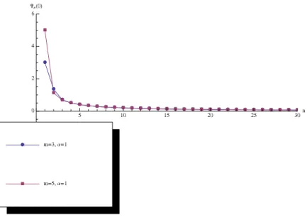
Finally, we exhibit the behavior of the Verblunsky parameters associated to the perturbation (22)for an absolutely continuous weightσdefined by the F´ejer kernel as follows (see [16])
dσ = 1 N+1 zN+1−1 z−1 2 dθ 2π
whose MOPSΦn(z), 0⩽n⩽N+1,N =0,1,2, . . .are given by Φ0(z)=1 Φn(z)= 1 2N−n+3 − 2N−n+2 2N−n+3z n−1+zn, 1 ⩽n⩽N+1.
ForN=30,Fig. 3shows the behavior of the perturbed Verblunsky coefficients for several values ofmandα.
Fig. 2. Behavior of Verblunsky coefficients for perturbations of the Bernstein–Szeg˝o measure.
Fig. 3. Behavior of Verblunsky coefficients for perturbations of the F´ejer Kernel.
Acknowledgments
The authors are grateful to the valuable comments of the anonymous referees. They greatly contributed to the improvement of this manuscript. The works of the first and third authors have been supported by Comunidad de Madrid-Universidad Carlos III de Madrid, grant MTM2009-12740-C03-01.
References
[1] A. Cachafeiro, F. Marcell´an, C. P´erez, Lebesgue perturbation of a quasi-definite Hermitian functional. The positive definite case, Linear Algebra Appl. 369 (2003) 235–250.
[2] M.J. Cantero, L. Moral, L. Vel´azquez, Polynomial perturbations of hermitian linear functionals and difference equations, J. Approx. Theory (2011)doi:10.1016/j.jat.2011.02.014.
[3] K. Castillo, L. Garza, F. Marcell´an, Linear spectral transformations, Hessenberg matrices and orthogonal polynomials, Rend. Circ. Mat. Palermo (II) 82 (2010) 3–26.
[4] K. Castillo, L. Garza, F. Marcell´an, Perturbations on the subdiagonals of Toeplitz matrices, Linear Algebra Appl. 434 (2011) 1563–1579.
[5] L. Daruis, J. Hern´andez, F. Marcell´an, Spectral transformations for Hermitian Toeplitz matrices, J. Comput. Appl. Math. 202 (2007) 155–176.
[6] L. Garza, J. Hern´andez, F. Marcell´an, Orthogonal polynomials and measures on the unit circle. The Geronimus transformations, J. Comput. Appl. Math. 233 (2007) 1220–1231.
[7] Ya.L. Geronimus, Polynomials orthogonal on a circle and their applications, in: Amer. Math. Soc. Transl. Series, vol. 1, Amer. Math. Soc., Providence, RI, 1962, pp. 1–78.
[8] Ya.L. Geronimus, Orthogonal polynomials, in: Two papers on Special Functions, in: Amer. Math. Soc. Transl., Series 2, vol. 108, Amer. Math. Soc., Providence, Rhode Island, 1977, English translation of the appendix to the Russian translation of Szeg˝o’s book [18], Fizmatzig, Moscow, 1961.
[9] E. Godoy, F. Marcell´an, An analogue of the Christoffel formula for polynomial modification of a measure on the unit circle, Boll. Unione Mat. Ital. 5-A (1991) 1–12.
[10] E. Godoy, F. Marcell´an, Orthogonal polynomials and rational modifications of measures, Canad. J. Math. 45 (1993) 930–943.
[11] U. Grenander, G. Szeg˝o, Toeplitz Forms and their Applications, 2nd ed., University of California Press, Berkeley, 1984, Chelsea, New York.
[12] E. Levin, D.S. Lubinsky, Universality limits involving orthogonal polynomials on the unit circle, Comput. Methods Funct. Theory 7 (2007) 543–561.
[13] X. Li, F. Marcell´an, Representation of Orthogonal Polynomials for modified measures, Commun. Anal. Theory Contin. Fract. 7 (1999) 9–22.
[14] F. Marcell´an, Polinomios ortogonales no est´andar. Aplicaciones en An´alisis Num´erico y Teor´ıa de Aproximaci´on, Rev. Acad. Colombiana Cienc. Exact. F´ıs. Natur. 30 (2006) 563–579 (in Spanish).
[15] F. Marcell´an, J. Hern´andez, Christoffel transforms and Hermitian linear functionals, Mediterr. J. Math. 2 (2005) 451–458.
[16] J.C. Santos-Le´on, Szeg˝o polynomials and Szeg˝o quadrature for the Fej´er kernel, J. Comput. Appl. Math. 179 (2005) 327–341.
[17] B. Simon, Orthogonal Polynomials on the Unit Circle, in: Amer. Math. Soc. Coll. Publ. Series, vol. 54, Amer. Math. Soc., Providence, RI, 2005.
[18] G. Szeg˝o, Orthogonal Polynomials, 4th ed., in: Amer. Math. Soc. Colloq. Publ. Series., vol. 23, Amer. Math. Soc., Providence, RI, 1975.
[19] C. Tasis, Propiedades diferenciales de los polinomios ortogonales relativos a la circunferencia unidad, Doctoral Dissertation, Universidad de Cantabria, 1989 (in Spanish).
[20] M.L. Wong, Generalized bounded variation and inserting point masses, Constr. Approx. 30 (2009) 1–15. [21] A. Zhedanov, Rational spectral transformations and orthogonal polynomials, J. Comput. Appl. Math. 85 (1997)