Elastic wave modes for the assessment of structural timber: ultrasonic echo for building elements and guided waves for pole and pile structures

1

Elastic wave modes for the assessment of structural timber: Ultrasonic echo

for building elements and guided waves for pole and pile structures

Martin Krause1*_{, Ulrike Dackermann}2_{, Jianchun Li}2

1_{Federal Institute for Materials Research and Testing (BAM), Division 8.2, Unter den Eichen 87,} 12205 Berlin, Germany

2_{Centre for Built Infrastructure Research, Faculty of Engineering and Information Technology,} University of Technology, Sydney, 15 Broadway, Ultimo NSW 2007, Australia

* Email address: [email protected], Tel.: +49 30 8104-1442, Fax: +49 30 8104-1447

Abstract This paper presents the state-of-the-art of using non-destructive testing (NDT) methods

based on elastic waves for the condition assessment of structural timber. Two very promising approaches based on the propagation and reflection of elastic waves are described. While the first approach uses ultrasonic echoes for the testing of wooden building elements, the second approach uses guided waves (GW) for the testing of timber pole and pile structures. The basic principle behind both approaches is that elastic waves induced in a timber structure will propagate through its material until they encounter a change in stiffness, cross-sectional area or density, at which point they will reflect back. By measuring the wave echoes, it is possible to determine geometric properties of the tested structures such as back walls of timber elements or underground lengths of timber poles or piles. In addition, the internal state of the tested structures can be assessed since damage and defects such as rot, fungi or termite attacks will cause early reflections of the elastic waves as well as it can result in changes in wave velocity, wave attenuation and wave mode conversion. In the paper, the principles and theory of using elastic wave propagation for the assessment of wooden building elements and timber pole/pile structures are described. The state-of-the-art in testing equipment and procedures are presented and detailed examples are given on the practical application of both testing approaches. Recent encouraging developments of cutting edge research are presented along with challenges for future research.

Keywords Elastic wave, ultrasonic echo, SAFT (Synthetic Aperture Focusing Technique), guided

wave, timber structure, timber pole, impulse response, condition assessment

1 Introduction

The non-destructive testing (NDT) of timber structures is important for i) the quality assurance of new construction works, and ii) the monitoring and health assessment of in-situ structures. For both applications, NDT methods are well suited to determine the current state of the tested structures.

In the present paper, the state-of-the-art of applying echo methods based on elastic wave modes for the assessment of timber building elements and pole/pile structures is presented. For this application, ultrasonic echo methods and guided wave (GW) methods that are already successfully used for concrete elements may be partially adopted.

For ultrasonic echo methods, the conventional procedures for concrete (an inhomogeneous material) demand ultrasonic techniques in the low frequency range. Timber structures, which are often made from glue laminated timber, have highly anisotropic elastic properties that must be considered in the ultrasonic echo testing and analysis. In order to obtain back wall echoes in sound timber, shear wave point contact transducers can enable the transmission of polarized wave modes without using a coupling agent. The disadvantage of large angle radiation may have an advantageous use for synthetic aperture imaging methods. The application of ultrasonic imaging by means of Synthetic Aperture Focusing Techniques (SAFT) is currently under test at a timber bridge for research.

2

For GW methods for pole/pile structures, traditional methods for concrete piles demand an impact excitation either from the top head or top side of the structure, which for timber poles/piles, is mostly not possible. In addition, the orthotropic nature of timber results in highly complex wave propagation with wave mode conversion and dispersive effects. While modifications of the conventional GW methods can be applied to timber pole and pile structures, their results may be inconclusive and inaccurate due to several complicating factors. The application of advanced signal processing techniques such as continuous wavelet transform, predictive deconvolution and machine learning may, however, provide solutions to some of these challenges.

The paper is organized as follows: in part A, the state-of-the-art of ultrasonic echo methods for building elements is described, and part B deals with GW methods for pole and pile structures. Each chapter summarizes the basics of wave propagation theory in timber, measuring equipment and handling, as well as examples of application.

A) Building elements investigated applying ultrasonic echo methods

The first part of this state of the art report describes non-destructive testing via ultrasonic echo methods. This is a rather new approach, which has started at Technical University Berlin and BAM with a diploma work in 2002 [1]. In order to understand the current state of the art in section 1 the theory of wave propagation in timber is summarized considering its strongly anisotropic behaviour in wood, whereas section 2 summarizes the existing measuring equipment and evaluating possibilities including ultrasonic imaging. In section 3 examples of results from research work and practical application on site are described

2 Physical principles and theory

2.1 Elastic wave propagation and reflection

Building elements made from timber have principally three axes of symmetry as depicted in figure 1: Longitudinal (L), Tangential (T) and Radial (R), where L is the direction of the fibres and R and T correspond to the current angle relative to the annual rings.

There are two approaches to apply ultrasonic echo methods for timber: One is rather simple in using the adequate instruments, whereas the second one needs to take into account the full anisotropic elastic properties of wood.

In the first approach, shear waves are used propagating in R and T-direction that means at right angles to the fibre direction L, having the polarisation in L-direction. These two wave modes have a large penetration depth in sound timber allowing to measure a clear back wall echo up to large depths (0.5 m and more). Shadowing effects of the back wall echo may indicate suspicious areas caused e.g. by fungi decay or insect attack. This method was developed since 2003 during several research projects [2, 3, 4].

Fig. 1 Timber beam (dimension: Naming of axes of symmetry in timber: Longitudinal (L~X1), Radial (R~X2), Tangential (T~X), image cited from [3] (left). Small specimen as used for specimens of glue laminated timber with quasi homogeneous anisotropic conditions (negligible curvature of annual rings) (right).

3

A 2nd _{possibility is to use ultrasonic imaging methods by means of synthetic aperture focusing} techniques (SAFT) in the low frequency range, as it is frequently applied for ultrasonic testing of concrete elements being an inhomogeneous but acoustically isotropic material [4]. The main requirement to do so is to consider the full angle dependent anisotropic behaviour of elastic wave propagation, as it is described e.g. in [6, 8].

The modelling of wave propagation and reconstruction calculation in this field is still under research and development with first applications for real structures. For investigating this, specimens from homogeneous anisotropic conditions are used (figure 1 right).

In the following paragraphs the basic knowledge of the two approaches is briefly summarised. 2.1.1 Elastic wave propagation and reflection in timber along axes of symmetry

Elastic wave propagation in timber is determined by its anisotropic properties. In a first approach there are three different directions of propagation corresponding to the 3 axes of symmetry: Longitudinal (L), Tangential (T) and Radial (R), where L is the direction of the fibres, where as R and T correspond to the currently valid angle relative to the annual rings (figure 1).

In a first simplified approach ultrasonic wave propagation on timber is described in an orthorhombic symmetry, without considering the curvature of the angular rings. An approach in order to determine the elastic constants is then to measure the ultrasonic velocities under approximate homogeneous anisotropic conditions. This means to measure ultrasonic velocities e.g. in small specimens.

In isotropic media, there are two elastic wave modes: pressure wave and shear waves. As in anisotropic media the polarisation of the shear waves relative to the symmetry axes has to be respected, there are principally 9 velocities propagating in the 3 axes of symmetry:

Vik : VLL, VRR, VTT, VRL, VRT, VTL, VTR, VLR, VLT where: i= L, R, T are the 3 axes of symmetry and

k = L,R,T are the three directions of the shear wave polarisation

In a similar manner, the different wave modes are indicated in the way that the first index indicates the direction of the wave propagation whereas the 2nd _{index indicates the direction of the polarisation.}

In this nomenclature VLL, VTT, VRR mean the pressure wave velocities (Vp), when the direction of polarisation is consistent with the direction of propagation. To give some examples: VLL stands for the p-wave velocity in direction of the fibres. Furthermore VTL means the shear wave velocity Vs of the TL shear wave mode propagating in T-direction with the polarisation in L-direction, whereas VLT is the velocity of the shear wave mode propagating in L-direction being polarised in T-direction.

Systematic experimental results on angle dependent velocity in wood were published between 1996 and 2002 by V. Bucur and co-authors [6, 7, 8]. Experiments at pine wood result in precise velocity values of all 3 wave modes in all symmetry axes. In order to achieve this immersion ultrasonic technique (p-waves) and piezoelectric transducers (s-waves) at cubic specimens having a edge length of 60 mm are applied. These results are published together with the effect of birefringence of the shear waves and an investigation of nonlinearity under uniaxial stress [7].

In case of spruce all velocities in symmetric directions were measured by means of ultrasonic transducers of 1 MHz mean frequency at cubic specimens of 16 mm edge length [8].

Transmission measurements at small specimens in the frequency range of 500 kHz to 2 MHz are also published in frame of a research work on through transmission measurement for application of tomography for spruce and pine trunks. This also includes transmission in off symmetry axes (see section 1.2.1)

Ultrasonic transmission measurements applying main frequencies of 500 kHz or 1 MHz are only feasible for specimens of low dimensions. For measuring ultrasonic through transmission or echo in real timber building elements, the attenuation of the elastic waves would be too high. This is caused by interfaces and inhomogeneities like knots and micro cracks.

4

In order to overcome these difficulties, low frequency ultrasound can be applied. For laboratory experiments at glued laminated timber this is feasible in the frequency range of 250 kHz shear wave transducers [10]. In applying low frequency p-wave transducers this was also successful for p-waves. Therefore broadband p-wave transducers were used being developed in the 1990ies for ultrasonic echo testing of concrete elements [2, 11]. As an example, Figure 2 presents the result of through transmission velocity measurement at pine wood for different locations relative to the annual rings. The measured velocity depends on the symmetry, but only measuring bar b4, indicating VRR and bars a1 and b1 indicating VTT are approximately fulfilling the condition of propagation along the axes of symmetry. For other sound paths, the results cannot be generalised because of the difference between group and phase velocity (see section 1.1.2).

Fig. 2 Velocity of longitudinal wave pulses for pine (main frequency 100 kHz) in dependence of

direction of fibre, (vRRl > vTT) [1]

Shear wave ultrasonic probes with dry coupling, which were successfully applied for ultrasonic imaging of concrete members, are successfully applied for ultrasonic echo measurement of timber since 2003 [1, 3]. Experimental work shows that these transducers can be successfully used for ultrasonic echo testing of structural timber in exciting both, the TL and the TR wave mode, respectively (see section 2.2)

The p-wave velocity in fibre direction is well known and can be used e.g. for pile length measurement, if the pile head is accessible. This wave mode is currently not used for beam like building elements. It is partly discussed in Part B of the present article in connection to bending waves.

As example Table 1 presents the velocities of the mostly applied wave modes for spruce for different frequencies found by different authors.

Generally it has to be stated that in large specimens exact velocity measurement by through transmission along the axes of symmetry in many cases is only successful for p-waves. This follows from the fact that transit time measurement is typically read from the first arrival of the transmitted pulse. When slower wave modes like VRL or VTL have to be measured, the first arrival of the transmitted pulse is often hidden by faster wave modes exited by the same transducers [13].

velocity [m/s] v e loc it ys [m/s]

5

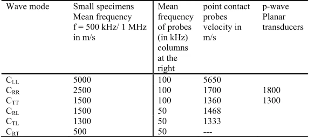
Table 1 Velocity of elastic waves in pine (Typical values from literature for different specimens and

frequencies)

Wave mode Small specimens Mean frequency f = 500 kHz/ 1 MHz in m/s Mean frequency of probes (in kHz) columns at the right point contact probes velocity in m/s p-wave Planar transducers CLL 5000 100 5650 CRR 2500 100 1700 1800 CTT 1500 100 1360 1300 CRL 1500 50 1468 CTL 1300 50 1333 CRT 500 50

---The comparison of the measured velocity shows rather large differences for identical wave modes. This is caused by individual differences of material properties, but is probably also due to the difficulty to make a clear distinction between the different wave modes. Investigations on the influence of different influencing factors on the velocity, such as frequency, dimensions of specimen relative to wavelength and homogeneity of the material have to be carried out at identical specimens of the same type of wood. Also the uncertainty of measuring the time of flight has to be taken into account.

The probability and intensity of wave propagation may not be deduced from the measured velocities. This depends strongly on direction of propagation. In order to know this, modelling of wave propagation following the elastic theory has to be performed (see below). The velocities are also measured in oblique-angled axes in order to determine the three dimensional off diagonal stiffness parameters (see section 2.2.1.).

Since the wave velocity of the shear wave modes RL and RT are rather similar in the low frequency range around 50 kHz, the angle between the propagation direction and the annual rings is less important. That is the reason why these wave modes can be used very successfully for non-destructive testing of timber and glue laminated beams (more details see Section 2.1 and 2.2)

Therefore this method is frequently used, and point contact transducers allow fast measurement without necessity to use any coupling agent (see section 2.1)

2.1.2 Reflection of Ultrasonic wave pulses

Shortly described, ultrasonic echo method means to measure the time of flight of elastic pulses, which are reflected at internal interfaces or internal objects. From the measured time of flight and the pulse velocity known from calibration measurements, the depth of the scatterers and interfaces can be deduced. Pressure waves (p-waves, longitudinal waves) as well as shear waves (s-waves, transverse waves) are used for non-destructive testing in numerous applications, in most cases in the frequency range of several megahertz and higher. Especially for the application in civil engineering, low frequencies are applied, because they enable high penetration depths in building materials. For concrete and timber building elements typical frequency range is from 25 kHz to 150 kHz.

Generally the wave propagation velocity for a monochromatic wave (phase velocity) can be written as:

c = λ * f (1)

6

For timber pressure waves as well as shear waves are applied. To give two examples, for a 100 kHz p-wave in the longitudinal direction of a pine specimen (typical velocity c = 5000 m/s) the wavelength results in = 50 mm, whereas a shear-wave of f = 50 kHz propagating in radial direction R (typical velocity VLR = 1400 m/s) has a wavelength of  = 28 mm.

The reflection R of p-waves at planar interfaces depends on the difference of the acoustic impedance between two materials. The acoustic wave impedance is a material property defined as the density ρ multiplied by p-wave phase velocity.

Zp = cP (2)

Then the reflectivity is

) 1 ( ) 2 ( ) 1 ( ) 2 ( P P P P z z z z R    (3)

where z is the acoustic impedance z in material 1 and 2, respectively.

In the case of shear waves the principle of the acoustic impedance is similar, but in this case the characteristic shear wave impedance has to be applied (cS: shear wave velocity) [13].

ZS = cS (4)

Then, in the case of the mostly applied horizontal polarised shear wave mode (SH), the reflection coefficient is similar to that of p-waves, but has opposite sign:

) 1 ( ) 2 ( ) 1 ( ) 2 ( S S S S z z z z R     (5)

Since the acoustic impedance of air can be neglected compared to timber or other building materials, the reflection coefficient at air interfaces is R = 1. When the impedance of material 2 is greater than for material 1, the sign of R is positive. When the acoustic impedance of the material 2 is smaller than for material 1, the sign of R is negative, that means that a phase jump of = 180° appears for the reflected wave pulse. This effect allows principally distinguishing between the reflection at a timber/steel interface and reflection at the timber/air interface because of its difference in the phase value. For prestressed concrete elements this effect is applied to indicate grouting defects in tendon ducts [15]. For timber elements this effect might principally be used for testing glued anchors or connecting sheets.

Generally ultrasonic pulses are produced and measured by means of piezoelectric probes. Thus the measured AC voltage for pressure waves is proportional to the sound pressure Ps in the material, which is defined by:

Ps = c= z  (6)

where z is the acoustic impedance (see Eq. (3), is the angular frequency (with = 2 f ) and  is the amplitude of particle oscillation.

For small timber specimens (length of the edge in the order of 100 mm), also relatively high frequencies like 0.5 or 1 MHz may be applied. But the development of ultrasonic echo applications for real building elements made from timber is based on frequency probes having a centre frequency of around 100 kHz, which must transmit broadband pulses. After basic research for ultrasonic testing of

7

concrete in the 1990’s, transducers and equipment were developed, which allow large area automated measurement and evaluation by reconstruction calculation and imaging [15, 16].

The ultrasonic echo method has the potential to locate and identify discrete defects or objects if sufficient focusing is achieved by the transducers. Because building elements made from timber usually contain inhomogeneities like knots or small cracks, structural noise may appear in the measuring curves reducing significantly the signal to noise ratio.

In order to overcome this problem, special transducers and imaging methods based on array techniques and synthetic aperture are applied. They have originally been developed for ultrasonic 13testing of concrete elements (and are continuously improved) in research and development activities [17, 18, 19, 5]. Some applications for timber are described in section 2.4.2.

2.2 Elastic wave propagation and reflection considering the full angle range

The basic ultrasonic testing procedure for, e.g. homogeneous steel specimens component parts made from steel, is to transmit a focussed ultrasonic beams having a well defined polarisation in a well defined direction and to register the echo from a reflector of interest. The distance into the known emitting angle then follows from multiplying the measured time of flight and the well known homogeneous wave speed of the material. For ultrasonic testing of timber elements none of the described conditions would be fulfilled:

a) Because anisotropy, neither the wave energy of the of an transmitted nor of a reflected pulse will in general have the same direction as the initiated pulse relative to the surface (following from the difference between phase and group velocity, see section 2.2.1).

b) The dimension of probe diameter and wavelength of ultrasonic waves will be in the same order of magnitude that results in the fact that the emitted and reflected pulse will cover a broad angle range.

In consequence the classical ultrasonic echo methods are not applicable for timber elements, except for wave propagation following the symmetry axes. This is the reason for discussing briefly the basics of wave propagation in timber (this section) and approaches for ultrasonic imaging applying the concept of synthetic aperture (section 2.2.2).

Since remark b) leads to successful application of ultrasonic imaging it seems obvious to adapt synthetic aperture techniques from concrete to timber. The principally broad angle characteristics of low frequency ultrasonic transmitter and receivers may be ideally used for broad angle sounding and synthetic focusing procedures afterwards. Since timber is anisotropic, one possible concept would be modelling the wave propagation in the frame of back propagation of measured ultrasonic A-scans (inverse propagation of wave fields in accordance with Huygens principle [19]).

As mentioned above and depicted in figure 1 right, the wave propagation is first discussed under homogeneous anisotropic conditions meaning that the curvature of the annual rings is neglected for the timber elements in focus.

2.2.1 Elastic properties of timber and wave propagation in orthotropic symmetry (Theory)

In a first step the anisotropic properties of timber are discussed in quasi homogeneous conditions meaning that the curvature of the annual rings could be neglected (see figure 1 right).

The fundamental elastodynamic equations describing the propagation of elastic waves in anisotropic media are based on the combination of Newton’s law (Newton-Cauchy) in three-dimensional tensional notation and the generalised Hooke’s law. Basic explanations and derivation of these elastodynamic properties in relation with respect to ultrasonic testing can be found in the research works cited in the next paragraph or in schoolbooks like [13].

Extensive theoretical approaches on elastic properties and wave propagation in wood are known since the publications by Musgrave (1960) [34] and Bucur [6, 29]. Later this was applied and updated by several PhD works and research projects by e.g. by Schubert [9], Chinta [20] and Krause [12].

The basic equation for describing the elastic behaviour is Hooke’s (or Cauchy-Hooke’s) law describing the relation between the mechanical Tension (T) and the strain (S):

8 T = c * S Where T: Tensor of tension c: Tensor of stiffness S: Tensor of strain _                   66 55 44 33 32 31 23 22 21 13 12 11 0 0 0 0 0 0 0 0 0 0 0 0 0 0 0 0 0 0 0 0 0 0 0 0 C C C C C C C C C C C C (2.1)

The stiffness is a tensor of the fourth stage and reduces to 36 components because of consideration of symmetry. Finally in orthotropic (orthorhombic) symmetry the stiffness tensor C has 9 independent components (Equation 2.1. right).

They may be estimated by mechanical measurement (static stiffness tensor) (see in [35], [36], [37]) or from ultrasonic velocity and density measurement (dynamic stiffness tensor, see below).

From theoretical considerations it follows that there are three wave types (as in all anisotropic materials), one quasi p-wave (qP) and two quasi shear waves (qS). The prefix quasi means, that the polarisation of the waves is either not strictly parallel to the pressure wave propagation, neither it is strictly perpendicular to the propagation direction as for pure shear wave modes. The stronger the anisotropy is, the weaker is the relation between wave propagation and polarization. In wood generally the notation qP qS1 and qS2 are used for the quasi pressure wave and the two quasi shear waves, respectively. In timber the qS2 wave is mostly polarised perpendicular to the plane of incidence that means it is polarised out of plane.

In order to estimate the stiffness components of the stiffness tensor the propagation velocity of the wave pulses in timber elements has to be measured along the different symmetry axes in timber. This means it has to be measured in six principal axis and three inclined axes of 45 grd. 1 _{with knowledge} of the parameters the so called slowness curves can be calculated, which visualize the reciprocal function of the velocity.

It has to précised that the velocity represented in the slowness curves is the phase velocity, meaning the value of the velocity (or the reciprocal slowness, respectively) depending on the propagation direction in the wooden “crystal”. For measuring the reflection of ultrasonic waves, for instance at an inhomogeneity in a timber specimen, we have to respect the propagation of the wave energy in order to localize the reflector. The velocity of the wave energy is the group velocity (in a non-dissipative material) and is different from the direction of the phase velocity.

From the derivation of the elastodynamic equation it follows that the vector of group velocity is always perpendicular on to the slowness surface (that means parallel to the wave normal n.) This is

demonstrated in figure 3 (left) that shows as an example the slowness curve of spruce in the L-T plane together with unite vectors of group velocity at several points of the qS wave mode. It should be noted remarked that the arrows indicating the group velocity in the concave section of the slowness curve lead to a kind of ambiguity: Different wave vectors point into in the same direction. This illustrates the reason for the so called cusps in the representation of the group velocity depicted in figure 3 on the right.

9

Fig. 3 Slowness curve (left) phase velocity (centre) and group velocity (right) of spruce in the

L~v1/T~v3~ plane (from [20])

When comparing slowness surfaces and group velocities for timber published from different authors it can be remarked, that they have principally the same typical attributes as crossing points of wave velocities and cusps, but they are different in details. This probably follows from the fact that the authors might have used different stiffness tensors for calculating the graphs of velocities. As mentioned above the components of the stiffness tensor (eq. 2.1) may be deduced from mechanical experiments or different measurements of wave velocities. However, as timber being a natural material it might not seem to be realistic to use material constants from tables in order to perform accurate ultrasonic testing in practise (as it is the case e.g. for steel). In order to overcome these difficulties an approach of interactively adapting the stiffness components in optimising the image of known reflectors inside the wood specimen of interest was developed. Those known reflectors may be e.g. corners of the rear face or known built in parts. This software is part of the software system Inter-SAFT (interactive Inter-SAFT) and was developed during a research work [12].

Based on the theory just discussed the wave propagation and scattering effects in wood can be effectively realized using numerical modelling: Elastodynamic Finite Integration Technique (EFIT) [30].This a numerical tool developed for the non-destructive testing of inhomogeneous isotropic and anisotropic materials. There are many applications in studying wave propagation and reflection in building elements as concrete [5] and, recently, wood [21]. It is also the requirement for applying reconstruction algorithms using elastic waves in timber (see section 2.2.2).

In figure 4 an example of wave propagation in spruce is demonstrated as snapshot from an EFIT movie after shear pulse excitation polarized in L-direction [20, 12].

10

Fig. 4 Snapshot of wave propagation in spruce after excitation of wave pulse Calculated with

3D-EFIT [21] applying stiffness parameter from [29]

2.2.2 Synthetic aperture imaging by means of synthetic data

Before applying reconstruction principles on experimental data, it was developed and tested using synthetic data. It is demonstrated in the following for wave propagation in the LT-plane of spruce, summarizing recent research work [19, 20, 21].

The geometry consists of circular Dirichlet scatterers (circular defects) with varying distance between them. A vertical excitation i.e. orthogonal to the fibre direction is applied. 2D-EFIT time domain snapshots are displayed in figure 5. It can be observed that a large part of the energy of qS1 wave is reflected by the inhomogeneities.

Fig. 5 2D-EFIT time domain snapshots of elastic wave propagation in the LT-plane (xz-plane: z-axis

corresponds to tangential axis (T) and x to longitudinal axis (L) which is fibre orientation direction) (from [20])

The synthetic data shown in figure 6a are obtained by EFIT simulation for a pulse-echo experiment. They are used for reconstruction of the defects. For reconstruction with isotropic SAFT each A-scan on the measurement surface is back projected into the material applying an isotropic (circular) travel time profile (here 1050 m/s, see figure 6b). The indistinct result of this SAFT reconstruction is shown

11

in 6b right. In contrast anisotropic SAFT using the qS1 group velocity (shown in figure 6c left) for back propagation succeeds in correct imaging the defects.

a) b)

c)

d)

Fig 6 Reconstruction of the scatterers from synthetic data. (from [20])

a) 2D-EFIT synthetic data, b) Left: Travel time profile used for isotropic SAFT, Right: Isotropic SAFT reconstruction with velocity 1050 m/s.

c) Group velocity used in anisotropic SAFT, d) Left: Travel time profile used for anisotropic SAFT, Right: Reconstruction with anisotropic SAFT.

3 Measuring Equipment, Visualisation of results and Imaging

In this chapter the basic information about the frequently applied measuring and evaluation techniques for timber is briefly summarized. This overview focuses on the low frequency application in order to obtain results of ultrasonic echo measurement for real building elements made from timber.

3.1 Measuring Equipment and Handling

For single point measuring, there are generally two types of equipment: transducers with planar contact on the measuring surface and dry contact transducers (point contacts). An instrument or development equipment contains four general features:

 A Electrical Pulse generation (AC Peak Voltage between 150 V and 1000 V)

 A piezoelectric transducer

 A receiving unit and an amplifier

 Displacement device of ultrasonic measuring curve (amplitude vs. time; A-scan) and indication of time of flight or reflector depth.

Transmitting / Receiving probes

Since the mid-1990s broadband transducers have been developed in the frequency range of 20 kHz to 300 kHz, for p-waves as well as for shear waves.

Low frequency shear and pressure wave transducers developed around the year 2000 have two main advantages: 1 The wave is directly generated by a ceramic tip pressed to the surface. There is no

12

centre frequency around 50 kHz (s-wave) and 100 kHz (p-wave). The polarisation axis of shear waves can be selected by the orientation of the device, thus SV and SH wave pulses can be excited [16]. Figure 7 depicts some examples of ultrasonic probes applicable for timber building elements. These are contact transducers requiring coupling agent, and point contact transducers, which are available as single transducers and transducer arrays in different arrangements. The frequency for the planar p-wave probes ranges from about 40 kHz to 200 kHz. The range of the point contact transducers is 70 kHz to 130 for the p-waves and 30 kHz to about 80 kHz for shear waves. That means the wavelength ranges around about 50 mm to 30 mm for the velocities around C = 2500 to 1300 m/s corresponding to the typically applied wave modes in timber (see table 1). The bandwidth of the probes is broad enough to obtain short ultrasonic pulses. For manual measurements an electronic interface can be used. The probe has twelve transmitting and twelve receiving transducers, which are working simultaneously.

Fig. 7Left: Broadband p-wave transducer 85 kHz .Centre: Point contact shear wave transducer (broad

band, 55 kHz centre frequency). Right: T/R probe with 12 transmitting (center) and 12 receiving (right) point contact transducers. Red arrow: Axes of polarisation .Yellow rectangle: Driven in the 1 transmitter – 1 receiver mode.

In a frame of a research project for testing the adhesive joints of glue laminated timber by ultrasonic echo measurement, shear wave planar probes were successfully applied by dry coupling [10].

For developing and optimizing low frequency ultrasonic techniques, often arbitrary pulses are applied. Typical equipment is shown in figure 8, in this case in application for a specimen made from concrete.

Fig. 8 Excitation of transmitting/receiving (T/R) transducer with arbitrary function generator, power

amplifier (not imaged) and oscilloscope (left). Principle sketch for working with arbitrary pulses and data processing (right).

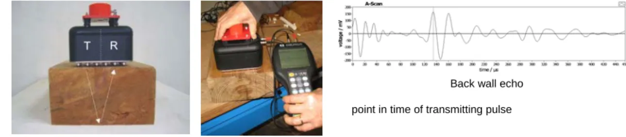
One of the commercially available instruments is depicted in figures 9, left and centre. It permits point measurement with preferable separate transmitter and receiving transducers as it is explained above and shown in figure 7. Since the transducer tips are made of ceramics, they are simply pressed at the measuring surface without any need of coupling agent.

The handling of the electronic part of the device in figure 9 is similar to the frequently used commercial equipment, which is applied for ultrasonic testing of steel in the frequency range between 1 MHz and 10 MHz. Figure 9, right, shows as an example a typical ultrasonic time curve (A-Scan, non

13

rectified, HF mode, see below) when the transducer is positioned above a tendon duct. The echo signals of the back wall is visible at t = 145 s (read at peak amplitude). From 0 s to about 40 s surface wave signals occur.

Single position thickness measurement of timber can be carried out with shear wave probes having the polarization RL of TL, as described in section 1.1. This is demonstrated in figure 9.

Fig. 9 Ultrasonic Echo Device with dry contact shear wave transducer (left) Handheld electronic

device (middle). Ultrasonic time curve (A-scan), non-rectified (HF-mode) (right).

For the purpose of enabling fast scanning of measuring surfaces with subsequent 3D imaging evaluation similar approaches applying point contact shear wave probes are developed [18]. With such systems either fast ultrasonic point measurement along lines or multistatic measurement is feasible. Linear Array

For fast measuring of surface areas there is an innovative device, which consists of 12 transducer modules. Each module consists of 4 parallels switched dry contact shear wave transducers (50 kHz as described above). The polarization axis is orientated orthogonal to the longitudinal axis.

The transducers and the electronics are mounted in a handheld box easily to be applied at concrete surfaces. The 12 transducer lines are switched as a multistatic array, meaning that one line acts as transmitter, and all others as receiver, then the second as transmitter, and so forth as shown in figure 10 left. In this way the whole area below the array is equally treated with ultrasound.

The data transfer is organized in the way that the whole data set is measured and stored in less than one second per location. The data measured along the line are combined to one data set and evaluated with fast reconstruction calculation following the principle of synthetic aperture (Synthetic Aperture Focusing Technique, SAFT) (see also section 3.2.3).

This system was originally developed for fast ultrasonic testing of building elements made from concrete. Together with imaging technique, the scatterers and reflectors in the volume of interest can be analyzed quickly on site with cross and longitudinal sections, as well as depth sections and phase evaluation. Since the point contact transducers used are similar to those described above they may be applied in the same manner for timber elements: Wave propagation into R and T having a polarisation in L (RL and TL mode).

Fig. 10 Principle of multi static measurement by means of a Linear Array (left). Example of

application with linear Array imaging of Timber (right).

point in time of transmitting pulse Back wall echo

14 Other Measuring Methods

Laser vibrometer (interferometer) are frequently used instruments for picking ultrasonic pulses at surfaces. For wood this was done by through transmission measurements in order to characterise wave propagation in stems [9].

Recently air coupled ultrasound becomes applicable also in the low frequency area. Already in 2005 through transmission for localisation of defects in pine specimens applying air coupled ultrasound in the frequency range of 100 kHz was demonstrated. This technique is now applicable for ultrasonic echo measurement of planar concrete elements [23]. In a thesis from ETH Zurich through transmission of air coupled ultrasound was applied also for slanted sound passes, which describes the future possibility for through transmission tomography [24].

3.2 Visualisation of Results

3.2.1 Naming conventions in ultrasonics

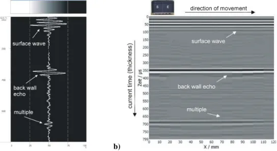
In technical language the visualisations of ultrasonic measurement results are named A-scan, B-scan and C-scan. To say with usual words, these are respectively: the ultrasonic point measurement in the time domain (A-scan), an ultrasonic cross- or longitudinal section (B-scan) or a depth section, parallel to the surface (C-scan).

Especially in low frequency ultrasonic technique, a more general application of the terms is used.

 A-scan: Amplitude of the measured signal vs. time (output voltage proportional to the sonic

pressure) vs. time. Three types of A-scans are used: HF-signal (not rectified), rectified and calculated envelope function. Figure 11 left shows the HF Signal of an echo measurement of a tendon duct in a concrete slab.

 B-scan: Amplitude of the time signal along the measuring (or a selected) axis showing the

depth information of the reflection (alternatively named: longitudinal or cross section of ultrasonic amplitude. It consists of a line (x-axis) of several A-scans and corresponds to the Radargram for Radar or sonogram of geophysical experiments. It is usually shown in a false colour (or grey scale) representation. The y-axis is either the time of the receiver after pulse excitation or the depth after calibrating the sound velocity (figure 11b).

 C-scan: Amplitude of the measured time signal along a plane parallel to the surface at a

specific depth (or time, respectively) showing the depth information. Alternatively named: depth section of ultrasonic amplitude. It corresponds to the “time slices” in case of Radar results.

15

a) b)

Fig. 11 Principle for controlling the homogeneity of a timber beam (idealized images measured at a

Polyurethane specimen)

A-scan with back wall echo and multiple (colour bar on top (black/ white) (left). B-scan measured stepwise with T/R-Probe (50 kHz shear waves) with back wall echo and multiple of the calibration specimen (right) (From [4]).

The basic principle for ultrasonic measuring and evaluation methods applied to material testing and medical diagnosis is focussing the ultrasonic wave field in a desired direction and distance. This is only feasible when the transducer wavelength is much larger than the wavelength in the material under investigation. Transducers that have a diameter in the order of the wavelength or smaller, produce a wave field with a large angle of aperture containing pressure and shear waves. Therefore scanning and imaging methods have a special relevance in low ultrasonic frequency applications.

The measuring procedure depends on the testing task. For instance, for thickness measurement of timber beams, simple point measurements with handheld equipment may be applied. But in most cases the evaluation of data requires imaging methods, which means that the data are measured almost along lines and are represented in B-scans.

3.2.2 Applicationsof use (B-scan visualisation) Gluelam compounds

In order to perform quality assurance of gluelam compounds, the use of ultrasonic echo technique was applied during a research project [25, 26]. In order to test the significance of ultrasonic testing, artificial defects like adhesive defects and cured adhesive layers are placed in specimens with thick glue lines. Defect edge length between 200 mm and 500 mm having gap width between 2.5 mm and smaller than 0.2 mm are realized in component thicknesses around 100 mm. The specimens are glued with typically applied adhesive, hydraulic pressure and pressing time.

Ultrasonic testing applying 250 kHz shear wave transducers permit to compare through transmission and echo measurements and presenting them in ultrasonic C-scans. For all specimens the ratio of echo and through transmission is compared. From the systematic study it follows that significance of the results depends on defect size and defect type, varying between missing adhesive, strip wise missing, and kissing bond.

In a subsequent research project point contact transducers were applied for the localisation of gaping joints, combined with measuring Finite Element modelling of angular radiation in gluelam specimens [27]. As a result it is derived that the method is applicable for some simple and few complex defects. However it has to be remarked that the modelling of wave propagation in this case

16

does not completely consider the anisotropic behaviour of timber, as it is described e.g. in section 2.2.1.

The capability to image a continuous adhesion defect in a gluelam beam (width 120 mm) is also demonstrated applying stepwise automated scanning with a point contact transducer (compare figure 9). The crack having a depth of z = 340 mm is significantly shadowing the back side echo of the beam, which is visible in the sound areas [4].

Bongossi bridges

After a damage of a Bongossi footbridge in 2008, special tests were carried out at numerous timber bridges in Germany. The reason was that the main supporting structure of the mentioned bridge was damaged by fungi attack without any externally visible signs.

Especially timber bridges crossing main roads have been in the scope of such investigations because of safety reasons. In the following one example is presented [quoted after 28]. It is a 30 years old, footbridge having longitudinal girder from Bongossi. Ultrasonic testing was carried out in the crossing region of longitudinal and cross girders. Figure 12 shows an example of an ultrasonic B-scan (longitudinal section). With exception of the region at the right hand (marked by an circle), the B-scan shows a sound back wall echo, the significance is demonstrated at the right showing the amplitude vs. time of the ultrasonic signal (A-scan). The conspicuous areas were tested by means of drilling resistance. In the present example the presence of fungi attack was confirmed, but its dimension was judged not to compromise structural safety [28].

Fig. 12 Ultrasonic testing of a footbridge made from Bongossi. Measurement along a line (B-scan)

and Ultrasonic signal at marked point indicating sound condition. Damaged region at the right (x = 30 … 40 cm) verified by drilling resistance (Image from [28], temporary copy, request for permission started).

This example demonstrates a very helpful combination of strict non-destructive and minor destructive methods. With ultrasonic testing the integrity of the structure may be verified, where as suspicious areas are localized and may be further investigated more precisely by means of more time-consuming methods.

3.2.3 Scanning and imaging techniques

In order to apply ultrasonic testing for concrete structures, there is a lot of experience using automated scanning systems. This technique can also be applied for timber structures with minor adaption work. As an example figure 13 depicts a scanning experiment applying a shear wave sensor head at a gluelam specimen from spruce with a scanning step width of 10 mm.

For ultrasonic testing of glue laminated timber also 2D-scaners are applied. Areas of one to two square meters may be scanned having a typical step width of 20 mm. Since the location of the scanner

Location on measuring axis Amplitude (HF-Signal)

de pt h in m m de pt h in m m

17

can be easily changed because of it’s fixing by suction foots, large areas can automatically be measured in relatively short time.

3D-Evaluation tools were developed for all types of data acquisition. In the current version of the reconstruction software, the important parameters such as wave velocity and opening angle can be selected interactively (program system Inter-SAFT [31]).

In order to realize this SAFT-reconstruction for wood, the reconstruction calculation is realized applying the slowness and group velocity curves describing the anisotropic sonic wave propagation in wood. On the base of these values the velocities can be interactively changed corresponding with the correct locations of known reflectors applying the features of inter-saft. This replaces the necessity to use values taken from literature in order to perform reconstruction calculation [32].

In figure 14 one example of imaging results is presented. The specimen made from spruce (size: 50cm x 40cm x 9cm), for symmetry. Circular disc shaped reflectors are realized via flat bottom hole. The measurement was done with a scanning system driven in a 1 transmitter - 1 receiver probe (see figure 7, right) exciting 75 kHz pressure waves in T~z direction.

Figure 14 depicts representative slices and projections from the result of 3D reconstruction by InterSAFT. As the comparison with the sketch of the specimen (Fig 14 right) shows, reflectors no. 1 to 5 and 11 are exactly imaged. The reason why the positioned reflector no. 6 to 9 are not imaged is not yet well understood. It is indeed true that they are positioned below a glued joint in the specimen, (depth z = 45 mm), but since the back wall echo is clearly measurable, the reason should not be a bad condition of the joint. It has to be noted that the back wall echo is nit clearly visible in the SAFT-B-scan depicted in figure 14, because it is reduced to the projection of the y-area of the circle slices.

Fig. 13 Automated scanner

working with shear wave point contact transducers as presented in figure 7 (right), transducer driven in the 1 transmitter – 1 receiver mode.

18 Linear Array

There are different evaluation procedures for the Linear array shown in figure 13 (2- and 3- dimensional). The 2-dimensional version is integrated in the system, as it is commercially available. It works quasi online for every location and is shown on the screen. For the 2-dimensional evaluation there are two approaches.

 One evaluates all stored datasets applying SAFT reconstruction showing the 3D- envelope function of the reflectors [33]. This is sometimes named sampling phased array, although it isn’t a real steering of the sonic beam.

 In second approach, a 3D-SAFT reconstruction is performed for the whole dataset including phase evaluation. The data measured with the linear array can additionally be used for testing the transverse transmission through different lamellas in gluelam [31]. As example we present a result obtained at a pedestrian bridge (object of study). It is constructed of Siberian larch gluelam. The measurement was done with a scanning system similar to that shown in [32] and also with the linear array described above. For the SAFT-reconstruction the velocity was adapted in a so called elliptical approach using the interactive features of in the software.

A part of the result is depicted in figure 15. It is the SAFT-C-Scan (depth section parallel to the surface, depth: 103 mm). It indicates two reflectors in a depth of 103 mm. It is a repeated measurement seven moths after an initial result and shows a stable location of the reflectors. The experiment shows the capability of the measuring system to imaging reflectors in gluelam. In the present case the reflectors, which are probably vertical cracks in the lamellas, are not relevant for static consideration.

Fig. 15left: Segment of a footbridge tested by means of automated ultrasonic scanning echo with

indicated reflectors from ultrasonic imaging procedure (blue) OP: reference point for scanner location..

Right: Part of 3D reconstruction result obtained by Inter-SAFT: SAFT-C-scan in a depth of

z ~T = 103 mm indicating significant reflection amplitude.

B) Assessment of timber pole and pile structures using guided waves

The second part of this state-of-the-art report presents the non-destructive testing using guided wave (GW) methods for the assessment of timber pole and pile structures. This testing approach is based on the propagation of elastic waves (stress waves) along an elongated structure with final boundaries, and is used, in particular, for the assessment of non-accessible areas, i.e. the underground section of timber pole/pile structures. In the presented paper, section 4 gives a brief introduction on the need of GW testing for timber poles/piles, section 5 describes the principles and theory of applying traditional GW methods - the sonic echo/impulse response (SE/IR) method and bending wave (BW) method - to timber pole/pile structures, section 6 gives details on required testing equipment for GW testing,

Fig. 14 Imaging result for spruce specimen F245, Polarisation TT, result of the

3D-SAFT-reconstruction with elliptic velocity profile and 2D-3D-SAFT-reconstruction (x~L, y~R, z~T) Projection of the y-area of the circle slices (left). Sketch of location and depth of the inner reflectors of the spruce specimen results presented in figure 9 (right).

19

section 7 presents typical examples of using the SE/IR method and the BW method for the embedment length estimation and condition assessment of timber poles/piles, section 8 describes the limitations and challenges of applying GW techniques to timber poles/piles, and section 9 presents recent research developments on advanced GW testing and analysis techniques for the condition assessment of timber poles.

4 Background

The non-destructive assessment of timber pole and pile structures is of crucial importance for reasons of old age and ill “health” condition of many currently installed structures, concerns of public safety and reliability, and budget restraints of asset management authorities. Most commonly used timber assessment techniques, such as visual inspection [1,2], sounding [3], resistography [4-6] or drilling [2,7,8], are typically restricted to the assessment of freely accessible sections of the structure, and have therefore only limited use for the testing of pole/pile structures due to their inability to assess the underground section of a pole/pile, which is indeed the most critical and vulnerable section [9]. The limitations of the common inspection techniques led to the development of GW-based methods for the non-destructive condition assessment of pole and pile structures. GW methods are based on the propagation of elastic waves (stress waves) along elongated rod-like structures with well-defined boundaries. They are capable of detecting internal damage and of evaluating the condition of non-accessible areas such as underground sections of piles and poles including their length estimation. GW methods have originally been researched and developed for the testing of deep foundation concrete piles [10]. Since their first practical application in the 1960th_{, various types of GW-based methods} have been developed and include the following most commonly used methods: the SE method, the IR method and the BW method. Based on the successful application of these techniques to concrete piles, modifications of these methods have been developed for their use on timber poles and piles. As such, Anthony and Pandey used the principles of the SE and IR method with modified testing configurations for the length estimation of timber piles in bridges [11,12]. The BW method was successfully applied by the researchers Douglas and Holt [13,14] for length determination of timber piles. And Kim et al. [15] investigated the use of the BW method for the condition assessment and length estimation of timber bridge piles. Recent research undertaken by the University of Technology Sydney led to further modifications and advancements of the SE/IR and BW method for their application to timber utility poles [16-18,9,19,20].

5 Physical principles and theory

5.1 General GW theory and testing

GW testing is based on the propagation of elastic waves, which are induced to a structure by applying an impact or impulse to its surface (typically by applying a hammer hit) whereby a sudden pressure or deformation is generated. A GW arises when the smaller dimension of the waveguide (its width or its diameter) is of the order of magnitude of the wavelength. The disturbance propagates through the structure and is reflected back from changes in stiffness, cross-sectional area and density. The propagation behaviour of the GW is a function of the modulus of elasticity (MOE), the density (ρ), the Poisson’s ratio (ν), and the geometry conditions of the structure [10]. As damage and deterioration changes the structure’s properties, the wave propagation behaviour is altered, resulting, for example, in early wave reflection, reduced wave velocity, increased wave attenuation and wave mode conversion. By analysing GW signals through identification of wave velocities, wave reflections and resonant frequency peaks, GW methods typically aim to detect damage and to determine the underground length of a structure. The schematic testing principles of the most commonly used GW methods, i.e. the SE method, IR method and BW method, are depicted in figure 16.

20

Fig. 16 Schematic testing principle of (a) SE and IR method and (b) BW method.

For the SE and IR method, the testing procedure is identical and involves the longitudinal excitation of a pile/pole structure with an impact hammer (ideally delivered at the head centre of the test structure) to generate longitudinal compression waves (see figure 16a). The imparted waves travel down the structure until a change in acoustic impedance (a function of velocity, density, moisture content and cross-sectional diameter) is encountered. At this point, the wave reflects back and is recorded by at least one sensor that is attached to the structure in close proximity to the impact location. While the SE method analyses the measurement data in the time domain, the IR method processes the data in the frequency domain. Both methods work best for the assessment of pole/pile structures with free access to the top of the structure. Modifications of the testing technique shave been developed to also enable the testing of structures with obscured access to the top. Both methods are suitable to assess structures with a ratio of underground length to diameter smaller than 20:1 to 30:1 [21], which is mostly given for timber poles and piles.

For BW testing, a transversal impact is applied to the pile/pole structure generating flexural/bending waves (see figure 16b), and wave signals are measured by multiple sensors located on the side of the structure. Thereby, the method is applicable for cases where the top of the structure is obscured such as bridge piles, foundation columns or utility poles for electricity and communication distribution. Since bending waves are highly dispersive in nature, dispersive analysis is required in which wave data is extracted from a selected group of frequencies.

5.2 Principles of SE and IR method for timber pole/pile assessment

For the condition assessment of timber poles and piles, both the SE and IR method can be applied to estimate the soil embedment length and to identify internal and underground damage/deterioration. Principles and details of both methods are described in the following sections.

The traditional SE method (also known as echo, seismic echo, sonic, impulse echo, pulse echo method and pile integrity test), is the earliest of all elastic-wave-based methods to become commercially available [22-24]. As mentioned above, the method operates in the time domain and analyses the reflection of longitudinal waves from the bottom of the tested structure or from a discontinuity (a change in acoustic impedance). The traditional IR method (termed also as sonic transient response, mobility, transient dynamic response and sonic method) is an extension to a technique originally proposed by Davis and Dunn [25] and is based on the elastic theory of cylindrical structures, which describes the relation of the wave reflection time to the resonant frequency of a structure. The technique operates in the frequency domain and evaluates dynamic resonance features of a pile/pole structure generated by longitudinal wave travel.

For both techniques, the first step in the data analysis procedure is to determine the velocity of the propagating longitudinal waves. Therefore, the times of the first arrival wave of two consecutive sensors of known distance are determined and the wave velocity is calculated according to:

a Impact Hammer b Sensor Pole/ Pile Soil Pole/ Pile Impact Hammer Sensor Soil Sensor

21    s V t (7)

where Δs is the spacing between two sensors and Δt the time difference between the first wave arrivals of the two sensors. To enhance weak echoes and to compensate for high soil damping, it is recommended to apply damping compensation techniques [26]. Thereby, damped signals can be retrieved and a clearer pattern of wave reflections obtained.

If only a single sensor is used for the testing, as for the traditional SE/IR testing, typical wave velocity values from the literature must be used. Table 2 lists typical ranges of the longitudinal wave velocities of different wood species depending on the moisture content. Due to the wide range of wave velocities in timber, the authors recommend to calculate the actual wave velocity of the test specimen from multiple sensors (see above) - large errors can occur when using wrongly predicted wave velocities from the literature.

Table 2 Longitudinal wave velocities of sound wood for different wood species

Wood species Longitudinal wave velocity _(m/s) Moisture content _(%) Reference

White Ash 3968–5076 12 Smulski [27]

Birch 4695–5747 4–6 Armstrong, Patterson & _{Sneckenberger [28]}

Yellow Birch 4348–5556 11 Smulski [27]

Black Cherry 4831–5435 4–6 Armstrong, Patterson & _{Sneckenberger [28]}

Douglas Fir 4926 10 Gerhards [29]

Sugar Maple 3906–5155 12 Smulski [27]

Red Oak 4425–5650 4–6 Armstrong, Patterson & _{Sneckenberger [28]}

Red Oak 3817–5000 11 Smulski [27]

Red Oak 3311–4425 12 Jung [30]

Southern Pine 5000–5882 9 Pellerin, De Groot & Esenther _[31] Yellow Poplar 5155–5747 4–6 Armstrong, Patterson & _{Sneckenberger [28]}

Sitka Spruce 5882 10 Gerhards[32]

For the SE method, the length of a pile/pole structure is derived from measurement data of a single sensor based on the time separation between the first arrival and the first reflection (echo) event according to [33]:  _   fw rw ( SE ) t l V 2 (9)

where l(SE) is the length of the structure, V the wave velocity calculated from Equation (7) or from literature and Δtfw-rw the time difference between the first wave arrival and the reflection wave. The actual embedment length can then be determined based on the calculated total length and the visible above-ground length of the structure.

For the IR method, the length is determined from frequency domain data. This can be done since the resonant frequencies of a pile/pole are related to the overall length of the structure. First, the time-history sensor measurement/s must be converted into frequency data using the using the fast Fourier

22

transform (FFT) algorithm [10]. If an impact hammer with a load cell is used for the testing (preferred), the Frequency Response Function/s (FRF/s) should be determined. Next, the resonant frequencies are identified from the FRF data. The pole/pile length can then be calculated from the wave velocity and computed frequency differences between the resonance peaks according to [25]:

   ( IR ) V l 2 f (11)

where l(IR) is the length of the pile/pole, V the wave velocity computed from Equation (7) or from the literature, and Δf the frequency difference between two resonance peaks in the FRF. The embedment length can again be calculated from the total length and the visible above-ground length of the structure. If the force of the impact hammer cannot be measured, resonant peaks and corresponding differences can also be determined using only the FFT/s of the sensor measurements.

Damage and/or deterioration can be identified through several indicators.

Multiple/early wave echoes in the measured time-history data indicate the existence of damage such as voids (e.g. from termite attack), cross-sectional changes or cracks. Principle: A change in acoustic impedance/discontinuity (change in stiffness or density) results in wave reflections.

A reduced wave velocity (calculated from wave arrivals of multiple sensors) compared to typical wave velocities from the literature, indicates the existence of timber deterioration such as rot or advanced fungi decay. Principle: Changes in the material properties such as high moisture content from rot result in slower wave propagation. Note: A slow wave velocity can also stem from generally high moisture content in the full structure. Measurement of the moisture content is therefore recommended before concluding an unsound state of the structure.

A large decrease in the amplitudes of the reflecting waves is a further indication of damage. Principle: Increased wave attenuation and wave mode conversion occurs due to wood deterioration such as rot or advanced fungi decay.

5.3 Principles of BW method for timber pole/pile assessment

The BW method is based on the travel of flexural/bending waves and can be used (similar to the SE and IR method) to determine the embedment length and to assess the internal and underground conditions of timber piles and poles [13,34,15]. Unlike the SE and IR method, the BW method analyses the propagation of flexural/bending waves (not longitudinal/compression waves). Since the impact is executed from the side of the structure opposed to its top, it is able to assess pile/pole structures where the top is obstructed or inaccessible. A challenge of the BW method is that flexural waves are highly dispersive in nature, which means that they are composed of many frequencies travelling at their own specific speed. Hence, the velocity of wave travel is not a constant, but a function of frequency (f) and wavelength (λ) [35]. A number of waves travelling together at their own individual velocity will therefore result in a constant change of the shape of the waves. To overcome the obstacle of wave dispersion, in the traditional BW method, the Short Kernel Method (SKM) is applied to identify the velocity of individual wave frequencies in the waveform and to thereby facilitate the data processing of the BW method [35]. The SKM is a mathematical technique based on the cross-correlation procedure described by Bendat and Piersol [36]. It was developed for digital signal processing and determines the velocity of selected frequencies inside dispersive time records. More details on the SKM can be found in [14].

To estimate the underground length of timber piles/poles using the BW method, wave patterns in the derived SKM plots of two sensors are analysed and characteristic features (positive or negative amplitude peaks) that are visible in SKM plots of both sensors are located and the amount by which this feature has shifted in time between the two sensors is determined. Similar to the SE method, this time shift is used to calculate the phase velocity of the selected kernel frequency according to Equation (7), where V is the phase velocity of the frequency from which the kernel is formed, Δs the distance of two sensors, and Δt the time difference between a feature (peak) of two sensors. The length of a test

23

structure is determined by identifying significant positive or negative amplitude peaks of the first arrival and the returning signals (reflections/echoes from an end of the specimen) in the SKM plot of a single sensor signal. By determining the time difference between the feature peak of the first signal and its corresponding peak in the return wave, the length of the pile/pole structure can also be calculated similar to Equation (9) of the SE method, where V is the computed phase velocity and Δt the time difference between a feature (peak) and the corresponding return feature.

The BW method can also be used to evaluate the soundness of timber pile/pole structures. The researchers Chen [2] and Qian [37] have found specific trends between wave speed and deterioration in timber piles. In general, a reduction in wave velocity indicates deterioration in timber. However, increased moisture content also results in a reduction in wave velocity, as shown by Ross and Pellerin [38], and must therefore be considered when using the BW method for the condition assessment of timber piles/poles. For preliminary soundness evaluation, Kim et al. [15] derived a chart based on in-field and laboratory data from timber piles that can be used for qualitative assessment of the integrity of timber piles/poles. In the graph illustrated in figure 17a, phase velocity data (determined from SKM plots) of intact and deteriorated timber poles are plotted against liquid content (LC) measurements. In their experiments, the researchers determined the LC using a Halogen Moisture Analyzer. This procedure gives a LC measurement which represents the true moisture content (MC) plus any additional volatile liquid (creosote) removal attributed to the heating process. Thereby, the assessment of treated wood is considered. Based on their data set, Kim et al. [15] established a divide, characterised by a 95% confidence interval, that distinguishes between intact and damaged pile data. This means, if measurement data falls below the 95% confidence interval, the tested pile is likely to be damaged while data above the dividing interval indicates an undamaged structure. Although some data points of externally damaged piles are located within the intact confidence interval of the graph, the chart is still considered as valid since the external damage would have easily been detected by visual inspection, making condition assessment based on GW redundant.

Fig. 17 (a) Relationship between phase velocity and liquid content for preliminary qualitative

condition assessment, and (b) condition evaluation chart for determination of RCSA (both graphs

adapted from Kim et al. [15]).

For ultimate quantitative condition assessment, Kim et al. [15] derived an equation that can be used to calculate their main cross-sectional area (RSCA) of a timber pile/pole based on phase velocity and liquid content measurements following:

-0.8294 450 723 e     p LC V RCSA (16)

where RCSA is the remaining cross-sectional area in %, Vp is the phase velocity in m/s and LC the liquid content. This relationship was derived by Kim et al. [15] from laboratory testing of timber piles. More detailed information on the derivation and calculation of the RCSA can be found in Kim et al.

24

[15]. Besides the empirical determination of the RCSA, the researchers also presented a condition evaluation chart that can be used to estimate RCSA values based on determined phase velocities and liquid contents. This chart, which was also derived from laboratory testing data, is illustrated in figure 17b. It is noted here, that while Kim et al. established the qualitative and quantitative assessment charts and equations using a reasonable large data set, uncertainties from different types of timber, natural wood defects and properties, temperature variations and soil properties will have influences on the wave velocity. Hence, these uncertainties must be considered when using the presented charts and equations. This is in particular important for quantitative assessment equation (16), which supposedly gives accurate values for up to one decimal point.

6 Testing equipment

The equipment required to perform GW testing consists of an impact hammer, multiple sensors (accelerometers), a multi-channel signal conditioner, a data acquisition system and a personal computer equipped with signal acquisition software.

6.1 Impact device

To generate guided waves in piles/poles, the structures must be excited by an impact device such as a hammer. For the SE method, an ordinary hammer is sufficient, while for the IR method and the BW method, a modally tuned impact hammer equipped with a load cell (see figure 18a) is beneficial to capture the force of the impact needed to calculate FRF data. An important feature of the hammer is the type of the hammer tip (hard, medium or soft). While hard tips produce high energy signals at high frequencies, soft tips generate lower energy signals at lower frequencies [12]. In general, it is important to execute an impact that produces a frequency spectrum that provides adequate information for GW analysis. For SE/IR testing, the authors recommend to generate an impact with a frequency range of up to 5000 Hz, while for BW testing, frequencies up to 3000 Hz should be excited. A higher excitation frequency bandwidth can also be achieved by mounting a steel plate (see figure 18b) or inserting a steel bolt (see figure 18a) to the timber pile/pole and inducing the hammer impact at the steel plate or steel bolt. To generate high quality wave data, the hammer impact should produce signals of minimal signal attenuation. The researchers Pandey & Anthony [12] found that a hammer of about 1.4 kg with a medium density plastic tip produces a good combination of signal energy with minimal signal attenuation for high quality signal data. For the SE/IR method, it is crucial to induce waves that are aligned primarily along the longitudinal axis of the pile/pole to generate mainly longitudinal waves. Hence, ideally, the impact is executed from the free top of the pile/pole structure. In practical applications, however, the top is often obscured by either a superstructure such as a bridge deck, or it is not accessible such as for utility poles with live electricity lines. In these situations, the impact must occur from the side of the structure. Therefore, it is recommended to use either a 90° impact bracket (see figure 18c) or a 45° steel bolt/lag screw (figure 18a) to provide an impact surface that allows the longitudinal excitation of the structure [12]. For the BW method, the impact can usually easily be imparted directly to the structure perpendicular to its longitudinal axis.

a b c

Fig. 18 (a) Modally tuned impact hammer (PCB HP 086C05) and steel bolt, (b) piezoelectric