Asymmetric and Non-Linear Adjustments in Local Fiscal Policy

Asymmetric and Non-Linear Adjustments in

Local Fiscal Policy

G

ABRIELLA

L

EGRENZI

CES

IFO

W

ORKING

P

APER

N

O

.

2550

C

ATEGORY

1:

P

UBLIC

F

INANCE

F

EBRUARY

2009

An electronic version of the paper may be downloaded

• from the SSRN website: www.SSRN.com

• from the RePEc website: www.RePEc.org

CESifo

Working Paper No. 2550

Asymmetric and Non-Linear Adjustments in

Local Fiscal Policy

Abstract

We analyse the revenue-expenditure patterns of local governments, allowing for asymmetric

and non-linear adjustments of local spending and taxation to disequilibrium errors. Our results

provide evidence of a downward inflexibility of both local government spending and local

taxation, pointing to a budget-maximising local government.

JEL Code: H10, H71, C22.

Keywords: fiscal federalism, fly-paper effect, non-linear time-series, asymmetric adjustment.

Gabriella Legrenzi

Department of Economics

School of Economic and Management Studies

Keele University

Staffordshire, ST5 5BG

United Kingdom

g.d.legrenzi@keele.ac.uk

February 13, 2009

A former version of this paper has been presented at the North American Summer Meeting of

the Econometric Society, at the annual meeting of the European Public Choice Society, and at

the annual congress of the International Institute of Public Finance. I would like to thank the

participants and discussants for their useful feedback. The usual disclaimer applies.

1

Introduction

The focus on …scal federalism and the potential role of local governments in dis-ciplining an excessive growth of public expenditure, has considerably increased in the recent years, following a remarkable growth of the public sector in indus-trialized countries. The debate on …scal federalism is even more pressing for the European Monetary Union member countries, given the budgetary constraints they are subject to.

Traditional public …nance analysis emphasizes the advantages of …scal de-centralization, as local governments have an informational advantage on central governments with respect to local costs and demand conditions, allowing them, under some conditions, to better satisfy local demands and deliver public ser-vices at a lower cost for public funds (see on this, Oates 1972, 1999). On the other hand, second generation models of …scal federalism point to the existence of con‡icting objectives between local and central governments, casting some doubts on the e¤ectiveness of …scal decentralisation (Oates, 2005). Besley and Coate (2003), in particular, introduce a political economy model where the con-‡ict of interests between central and local administrations results in excessive spending by local governments. The soft-budget constraint of local governments is also analysed in Kornaiet al. (2003).

In the light of the discussion above, it becomes very important to analyse more in detail the relationships among the spending and taxing decisions of local governments and the level of transfers received from higher levels of government. For this purpose, the empirical analysis on the revenues-expenditure patterns of local governments is traditionally based on the implicit assumption of symme-try: e.g. local expenditure is expected to increase and decrease symmetrically

following changes in unconditional transfers received and own resources. To the best of our knowledge, very few studies have considered possible asymmetries and non-linearities in local …scal policy, as in Gamkar and Oates (1996), Stine (1994) and Heyndels (2001).

Using annual time-series data for Italian municipalities, our paper examines the relationship between local revenues and expenditures in a non-linear frame-work. The analysis of Italy is of particular interest, not only because Italy is an EMU country, but also because it introduced some important reforms, where the country initially strenghtened its centralisation process, only to subsequently enhance the delegation of spending powers to local authorities.

There are two main di¤erences between our paper and the studies mentioned above. First, we use the Johansen (1988, 1995) multivariate cointegration tech-nique, which allows for long-run properties and short-run dynamics of local expenditure, taxation and state transfers to be jointly analyzed, allowing for possible endogeneity of the variables1_{. Second, we allow for asymmetric and}

non-linear adjustment to disequilibrium deviations of the …scal variables from their equilibrium levels, following the methodology introduced by Escribano and Granger (1998).

We …nd evidence of a "strong" ‡y-paper e¤ect, in the form of a high transfer-elasticity of local spending, associated with an insigni…cant long-run e¤ect of local taxation. This means that local spending is ultimately driven only by the size of transfers received, regardless of the ability of local governments to raise revenues from their own resources.

The adoption of non-linear modelling allows us to report asymmetric

ad-1_{Knight (2002) argues that transfers are the result of a political bargaining process and} therefore should be considered as endogenous.

justment, in the form of downward in‡exibility of both local expenditure and taxation. When local expenditure is below its equilibrium level with transfers, it raises relatively fast, while when it is below, its reduction is not statistically signi…cant. In the case of municipal taxation, taxes raise faster when they are below their equilibrium level, than they reduce when they are above.

Our empirical results therefore point to the existence of a budget-maximising local government, questioning the opportunity of further delegation of spending powers to local governments, when unaccompanied by a corresponding increase in their …scal responsibility and control over local spending.

The paper is organized as follows; the next section presents a short survey of the economic literature on the local revenue-expenditure models. Section 3 estimates the long-run relationships among local expenditure, transfers and taxes whereas section 4 reports the short-run equations allowing for asymmetric and non-linear adjustment. Finally, section 5 provides some concluding remarks and suggestions for further research.

2

Local Revenue-Expenditure Models and the

Fly-Paper E¤ect.

Traditional economic literature on the revenue-expenditure patterns of local gov-ernments has emphasised the existence of a "‡y-paper" e¤ect2. The ‡y-paper e¤ect refers to the empirical regularity that the transfers-elasticity of local ex-penditure is higher than its own-resources elasticity. It is important to consider that the ‡y-paper e¤ect is not an anomaly3 _{within the rational choice, as}

ar-gued by Hines-Thaler (1995), but, instead, it is a signal that local and central

2_{The term ”‡ypaper” is derived from the well-known remark by Arthur Okun that ”money} sticks where it hits”.

governments might have di¤erent (and potentially con‡icting) objectives. This happens because …scal discipline at a general government level has the charac-teristics of a non-excludable public good4_{. As a consequence, there is a common}

pool problem where local governments are incentived to overspend, to promote the interests of the local citizens/taxpayers, in the case of a responsive govern-ment, or of their elected politicians/bureaucrats in the case of a Leviathan-type of government5.

The costs of the ‡y-paper e¤ect (state transfers to cover local …scal unbal-ances, given the soft-budget constraint of local governments) will be shared at a national level, while its advantages will be internalized by the single jurisdic-tions. If the ‡y-paper holds, delegation of spending powers to local jurisdictions, unaccompanied by a corresponding increase in their …scal responsibilities, will have the e¤ect of expanding rather than contracting public sector size (Legrenzi 2000, Milas-Legrenzi 2002), as local governments are incentived to free-ride on the national …scal discipline.

The ‡y-paper e¤ect has received considerable empirical support in the lit-erature (Hines and Thaler 1995), but has generally being analysed under the assumption of symmetry.

Under the hypothesis of symmetry, the local government reduces its expen-ditures in response to reductions in transfers received, whereas in the presence of asymmetries, the local government might decide to enhance its capacity to raise revenues, in order to keep unchanged the level of local expenditure. This is the so-called positive …scal replacement hypothesis, and it is empirically supported

4_{At a general government level, the …scal discipline can be identi…ed in the compliance to} Maastricht and Amsterdam criteria for the EMU, while at a local level there is no such de…n-ition, although a local balanced budget would be desirable to achieve the nation’s budgetary ob jectives.

5_{For further information on the distinction between ”responsive” and ”excessive”} govern-ment, see Buchanan (1977) and Legrenzi and Milas (2002).

by Gramlich (1987), for the US. On the other hand, Paine and Stine (1994) identify a ”super ‡ypaper” e¤ect for a panel of Pennsylvania counties: when grants are cut, own revenues also fall, resulting in a negative …scal replacement. The …ndings of Gamkar and Oates (1996) for the US suggest that the ‡ypaper e¤ect operates in both directions, providing no support in favor of asymmetric behavior.

On the other hand, non-linearities may arise if the …scal authorities react di¤erently to deviations of state transfers from their equilibrium level. For instance, the local authorities may be more willing to raise taxes rapidly when they are below their equilibrium level with respect to transfers, rather than lowering taxes rapidly when these are above their long-run level.

In the context of the European Stability and Growth Pact, testing for asym-metries and non-linearities in the revenue-expenditure models becomes increas-ingly important for economic policy purposes, in order to evaluate reforms in the transfer system and the e¤ectiveness of decentralization in constraining the growth of government spending.

3

The Empirical Model.

We base our empirical analysis on the Italian municipalites. Italy is a member country of the European Monetary Union with a typically high level of public debt (around 122% of GDP in 2006), a high de…cit (4.6% of GDP in 20066), for which the control of public spending is particularly important. Increasing the authonomy of local governments is highly debated in the political arena, as a possible solution to constrain public expenditure growth. The …nancing of

6_{The data on the Italian de…cit and debt are taken from the 2005Annual Report of the} Italian Central Bank (Banca d’Italia).

local expenditure is heavily reliant on transfer-…nancing from the state, and the Italian Constitution links the levels of transfers granted to local governments to their "…nancing needs".

Italian municipalities are the lowest level of local government in Italy, being therefore closer both to the local preferences and the local costs conditions, with respect to the central government. They enjoy some degree of …scal autonomy, setting their own property taxes, and are responsible for the local public ser-vices provision (transport and public utilities)7. Another advantage deriving from the choice of the Italian municipalities derives from the policy switches in their …scal autonomy. The 1973 reform limited the taxing powers of the Italian municipalities, on the grounds of the higher e¢ ciency of a centralised tax collection system. On the other hand, the reforms of the 1990s enhanced the taxing powers of municipalities, increasing their autonomy, on the belief that this would help constraining the public expenditure and help the country to respect the EMU requirements8_{. An Internal Stability Pact was introduced}

in 1999, requiring to extend to local governments the European Stability Pact requirements, in the annual Budget Law. 9

Our sample consists of annual observations over the 1955-200310 _{period, and}

is taken from the Italian o¢ cial statistics from ISTAT, in real terms. Gmeasures

the expenditures of the Italian municipalities,T R the transfers received from

higher levels of government, andT AX the municipal taxation.

All the variables are expressed in logs. We chose annual data on the grounds of the annual frequency of the budgetary choices of local governments. Higher

7_{For more detailed information on the competencies of the Italian municipalities, see} Legrenzi (2000).

8_{For further information and analysis on the Italian reforms, see OECD (2005).}

9_{For a critical review on the reforms of the Italian …scal federalism, see Bordignon (2004).} 1 0_{The year 2003 is the latest available in the national statistics. The data from 2001 onwards} are nevertheless provisional.

frequency data will give us more degrees of freedom, but, nevertheless, will bias the analysis, given the annuality of the municipal budgets11_.

Levels and …rst di¤erences of the variables are plotted in Figure 1.

Preliminary analysis of the time-series properties of the data suggested that all variables are non-stationary in levels12 _{. Given the possible endogeneity}

among the variables in question, we employ the Johansen approach to cointe-gration. Following Johansen (1988, 1995), we write a p-dimensional vector error correction model as:

yt= k 1

X

i=1

i yt 1+ yt 1+ +"t (1)

whereyt= [G; T R; T AX]0is the set of non-stationary I(1) variables discussed

above,"t niid(0; ); is a drift parameter, and is a(p p) matrix of the

form = 0 , where and are(p r)matrices of full column rank, with

containing the r cointegrating vectors and carrying the corresponding loadings in each of the r vectors.

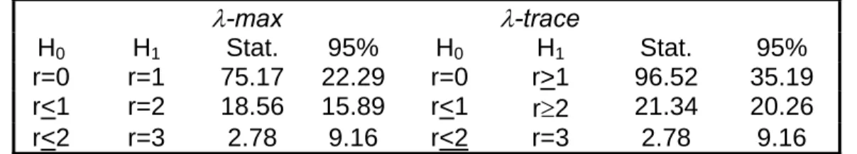
Allowing for an unrestricted intercept term and a lag length of k = 1 in the VAR model13_{, Table 1 reports the -max and the -trace test statistics}

for cointegration together with their corresponding 95% critical values (calcu-lations are done in Micro…t 4.1; see Pesaran and Pesaran, 1997, and in E-views 5.1). The empirical results provide evidence of two cointegrating vectors, which is stronger for the -max rather than the -trace statistic. We consequently proceed by assuming the existence of two cointegrating vectors. For exact

iden-1 iden-1_{A further di¢ culty arises since the municipal …scal year does not coincide with the calendar} year, which forms the basis of the municipal data collection.

1 2_{Results are available on request.}

1 3_{The k=1 is chosen by both the Schwarz information criterion and by the Hannan-Quinn} information criterion. The Akaike would have supported a lag lenght of 3. Given the small sample considered, we set k=1 to avoid the loss of too many degrees of freedom.

ti…cation we impose a unit coe¢ cient on municipal expenditure ( 11= 1) and

a zero coe¢ cient on taxes ( ₁₃= 0) in the …rst vector, and a unit coe¢ cient on municipal taxation ( ₂₃ = 1) and a zero coe¢ cient on municipal expenditure ( ₂₁= 0)in the second one. These restrictions are justi…ed on the grounds that, given the possibility of one cointegrating vector based on the tracestatistics,

we also normalized onGand tested for zero long-run e¤ects from taxes within

one cointegrating vector. This hypothesis was not rejected at conventional levels of statistical signi…cance14. This result motivates the exclusion of taxes from the …rst cointegrating vector as a valid identifying restriction. We have also tested for weak exogeneity of transfers for the rest of the system. This is a test on the adjustment (alpha, ) coe¢ cient on TR in the two cointegrating vectors. The test is a Likelihood Ratio (LR) test distributed as a 2_{(2) under the null,}

giving a value of 4.204, which is insigni…cant at the 5 percent level (p-value = 0.122). In statistical terms, weak exogeneity of transfers implies that we can proceed by estimating short-run equations forGandT AX conditioning onT R

without loss of any signi…cant information. In economic terms, conditioning on transfers has the interpretation that within current local government …scal pol-icy decision-making, state transfers are exogenous, con…rming our normalization choice.

Imposing the restrictions discussed above yields the following restricted cointegrating vectors:

G= 0:71T R(s.e.=.02) (2)

and

T AX= 0:50T R(s.e.=.03) (3)

The highly positive coe¢ cient of transfers in the …rst vector con…rms the existence of a ‡y-paper e¤ect: a 10% increase in state transfers raises municipal expenditure by 7%. The irrelevance of municipal taxation in determining lo-cal expenditure represents a peculiarity of the Italian municipalities, which we consider to be a ”strong” version of the ‡y-paper e¤ect. This means that the long-run equilibrium values of local expenditure are entirely driven by the level of transfers received from higher levels of government.

The second cointegrating vector describes the relationship between local tax-ation and state transfers. Local taxtax-ation in the long-run is expected to increase by 5% in response to a 10% increase in state transfers. This means that in-creases in state transfers do not bring tax relief to the community. In addition to the long-run analysis, further useful insight to understand the spending and taxing decisions of the Italian municipalities is provided in the short-run analysis below.

4

Short-run adjustments of local taxes and

spend-ing.

Having veri…ed the existence of a long-run equilibrium among the local …scal policy variables, we model their short-run adjustments conditioning on transfers. The two cointegrating vectors given by equations (2) and (3) above are denoted by CV1 and CV2, respectively. We initially estimate a linear error-correction

model for local expenditure and local taxation and subsequently test for possi-ble non-linearities. In case where the null of linear adjustment is rejected, we proceed by estimating non-linear error-correction models.

Various authors have examined non-linearities in the behavior of error cor-rection models (see e.g. Granger and Lee, 1989; Escribano and Pfann, 1998; Escribano and Granger 1998; and Escribano and Aparicio, 1999, among oth-ers). In particular, Granger and Lee (1989) partition the error correction term into its positive and negative components, and feed them back into the short-run dynamic equation. The idea here is to test for di¤erent speed of adjustments depending on whether the …scal variables are above or below their unique (at the zero point) equilibrium. However, imposing a unique equilibrium around zero may be too restrictive. In order to relax this assumption, Escribano and Granger (1998) and Escribano and Aparicio (1999) among others, use a cubic error correction term. This type of nonlinear adjustment is more ‡exible than the Granger and Lee (1989) type of asymmetric adjustment as it allows for the possibility of more than one equilibrium point. This type of non-linear adjust-ment also allows for a faster adjustadjust-ment when deviations from the equilibrium level get larger.

4.1

Short-run adjustments of municipal expenditure.

We initially estimate the error correction model on the assumption of linear response of municipal expenditure with respect to increases and decreases of State transfers from their equilibrium value. The model estimated is therefore:

Gt=C+ 1 T AXt+ 2 T Rt+ 3CVt11+ut (4)

We also considered an EMU dummy, taking the value of 1 from 1993 onwards, to capture the impact of the European Monetary Union, and a centralisation dummy, taking the value of 1 between 1973 and 1990, to capture the central-isation of tax collection under the 1973 reform. The Internal Stability Pact

is captured by a dummy taking the value of 1 from 1999 onwards. All these variables were statistically insigni…cant in all models.

Regression results are reported in Table 2(i). The linear model is rather poor, failing most of the diagnostic tests. This might be due to omitted non-linearities. To detect this, we initially test for linearity in the residuals of the error correction model. We apply the well known Brock, Dechert and Sheinkman (1996, thereafter BDS) test statistic. Under the null hypothesis of linearity in the residuals, the BDS test follows the normal distribution whereas rejection of the null implies an unspeci…ed non-linear structure15_{. Based on the p-values}

associated with the BDS test, the results in Table 3 suggest the presence of non-linear structure in the residuals of the error correction model.

Table 2 (columns (ii) and (iii)) reports the error correction equation based on di¤erent types of non-linear adjustment. First, as in Granger and Lee (1989), we take the deviations of lagged CV1around its mean value, and partition them

into their positive and negative components (denoted by CV+₁ and CV₁, respec-tively). Then, as in Escribano and Granger (1998) and Escribano and Aparicio (1999), we estimate a cubic error correction model. More speci…cally, we allow for lagged CV2

1and CV31to enter the short-run equation. The asymmetric model

takes the form:

Gt=C+ 1 T AXt+ 2 T Rt+ 3CV1+;t 1+ 4CV1;t 1+zt (5)

The non-linear model takes the form:

Gt=C+ 1 T AXt+ 2 T Rt+ 3CV1;t 1+ 4CV12;t 1+ 5CV13;t 1+et (6)

1 5_{Several non-linearity tests exist in the literature. However, as Ashley and Patterson} (2001, p.20) point out, the BDS test is the best among di¤erent tests for use as a non-linearity screening test.

The results in Table 2(ii) show the presence of an asymmetric adjustment for local expenditure that relies on a downward in‡exibility of this …scal policy variable. Indeed, the coe¢ cient associated with the lagged value of CV+₁ is statistically insigni…cant. This means that when local expenditure is below its equilibrium level with state transfers, it increases relatively fast, whereas when it is above its equilibrium, its reduction is not statistically signi…cant.

The non-linear ECM results, in Table 2(iii), provides some evidence of pos-sible non-linearities in the adjustment of local expenditure, given the statistical signi…cance at a 90% con…dence level of the CV2

1 (but not the CV31) regressor.

Therefore, there is some evidence of a faster adjustment when deviations from the equilibrium level get larger.

Next, we plot the asymmetric and non-linear types of adjustment against CV1(see Figure 2 and Figure 3, respectively). From Figure 2 there is evidence

of asymmetric adjustment as the cross-plot is far from being a straight line. The plot of the nonlinear cubic polynomial in Figure 3 suggests the existence of asymmetric adjustment around a unique equilibrium point.

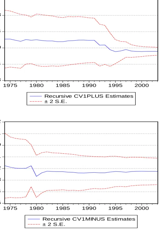
The recursive estimates of the asymmetric ECM for local spending, in Figure 6, verify the insigni…cance of CV+₁ as the estimates the 2 standard error bands always include zero. On the other hand, the recursive estimates for CV₁ suggest that the asymmetry gets stronger over time, in the sense that the point estimate starts from around -0.18 to reach -0.25 at the end of the sample.

4.2

Short-run adjustments of the local taxation.

We now report the ECM model for local taxation, allowing for possible non-linear and asymmetric behaviour. Results are reported in Table 4. As for local spending, we perform a BDS test on the residuals of the linear ECM. Based on

the p-values associated with the BDS test, the results in Table 5 strongly suggest the presence of non-linear structure in the residuals of the error correction model for TAX. Table 4(ii) and 4(iii) report the estimated error correction equation, based on the di¤erent types of non-linear adjustment discussed earlier. The CV+₂, CV₂, CV2

2 and CV32 variables are constructed in the same way as the

corresponding CV1regressors.

The results in Table 4(ii) demonstrate the presence of an asymmetric adjust-ment for local taxation that relies on a downward in‡exibility of this …scal policy variable. Indeed, the coe¢ cient associated with the lagged value of CV+₂ (i.e. -0.01) is lower than the coe¢ cient on CV₂ (i.e. -0.30), and it is also statistically insigni…cant. This means that when local taxes are below their equilibrium level with respect to state transfers, they increase relatively fast, whereas when they are above their equilibrium, they fall relatively slowly.

The linear ECM results in table 4(iii) show the existence of possible non-linearities in the adjustment of local taxes, backed by the statistical signi…cance of the CV2

2 (but not the CV32) regressors. Therefore there is evidence of faster

adjustment when deviations from the equilibrium level get larger.

Next, we plot the asymmetric and non-linear types of adjustment against CV2(see Figure 4 and Figure 5, respectively). From Figure 4 there is evidence

of asymmetric adjustment as the cross-plot is far from being a straight line. The plot of the nonlinear cubic polynomial in Figure 5 suggests the existence of one equilibrium.

The recursively estimated coe¢ cients of the asymetric ECM for local taxa-tion, plotted in Figure 7, show that the e¤ect of the asymmetry is stable over time.

by the Italian local governments, that the di¤erent reforms have so far been unable to tackle. A stronger link between municipal expenditure and municipal taxation, as well as spending and transfers reforms will be needed in order for decentralisation to e¤ectively constrain the growth of government spending in Italy.

However, some caution must be taken when interpreting the results above. The use of aggregate data has the e¤ect of lumping together the responses of all Italian municipalities, and therefore, the estimated response could re‡ect some mixture of symmetric and asymmetric coe¢ cients (Gamkhar and Oates, 1996). Further, the degree of asymmetry might also depend on some characteristics of the local jurisdictions, that cannot be captured by the aggregate data (Gamkar and Oates, 1996). Territorial distinctions can also be relevant for Italy, given the importance of state transfers to southern areas (see also OECD, 2005). On the other hand, as our main focus is on the macro-economic impact of local …scal policy, the use of aggregate data is necessary to assess the macro-asymmetries in the local revenue-expenditure models.

5

Conclusions

This paper models the local revenue-expenditure relationship in the case of Italian municipalities, using both linear and non-linear cointegrating techniques. The long-run analysis shows the absence of a direct link between local ex-penditure and taxation, as local spending is entirely driven by the amount of transfers received by the central government. The short-run asymmetric model shows evidence of revenue-maximising behaviour by local governments, driven by the downward in‡exibility of both local expenditure and taxation.

del-egation to local governments of further power to spend should be attached to a higher level of …scal responsibility, that is linking local expenditure to local taxation, in order for local governments to face an e¤ective budget constraint. If this were not the case, the decentralization of public expenditure might provide the undesired outcome of an expansion rather than contraction in public sector size, given the downward in‡exibility of both the local …scal policy variables.

Further, the downward in‡exibility of local expenditure appears to be a relevant problem in this context, that so far has not been explicitly tackled by the di¤erent reforms, evidenced by the insigni…cance of the policy dummies as well by the analysis of the recursively estimated asymmetric ECM coe¢ cients.

There are at least two possible extensions of our analysis. First, territorial and dimensional di¤erences might be captured within a panel data model of Italian municipalities. Second, it would be interesting to introduce and estimate a two-regime smooth transition autoregression model (STAR, see e.g. Granger and Terasvirta, 1993), where adjustment takes place in every period but the speed of adjustment varies on whether disequilibrium deviations are large or small. These issues can be addressed in future research.

References

[1] Ashley, R.A. and D.M. Patterson (2001). ”Nonlinear Model Speci…ca-tion/Diagnostics: Insights from a Battery of Nonlinearity Tests”, Eco-nomics Department Working Paper E99-05, VirginiaTech.

[2] Besley T. and Coate S. (2003). "Centralized versus Decentralized Provision of Local Public Goods: a Political Economy Approach",Journal of Public Economics 87: 2611-2637.

[3] Bordignon M. (2004), "Fiscal Decentralization: How to Harden the Budget Constraint", paper presneted st the Worksho "Fiscal Surveillance in EMU: New Issues and Challenges", Bruxelles, Novemner 2004.

[4] Brock, W.A., D.A. Hsieh and B.D. LeBaron (1991). Nonlinear Dynamics, Chaos and Instability, MIT Press, Cambridge.

[5] Brock, W.A., W. Dechert and J. Scheinkman (1996). A Test for Inde-pendence Based on the Correlation Dimension, Econometric Reviews 15: 197-235.

[6] Buchanan J.M. (1977) Budgets and Bureaucrats: The Sources of Govern-ment Growth, Duke University Press.

[7] Escribano, A. and F. Aparicio (1999). "Cointegration: Linearity, Nonlin-earity, Outliers and Structural Breaks" in Dahiya, S.B. (ed), The Current State of Economic Science, Spellbound Publications, Vol 1, 383-407. [8] Escribano, A. and C.W.J. Granger (1998). "Investigating the Relationship

between Gold and Silver Prices".Journal of Forecasting 17: 81-107. [9] Escribano, A. and G.A. Pfann (1998). "Nonlinear Error Correction,

Asym-metric Adjustment and Cointegration". Economic Modelling 15: 197-216. [10] Gamkhar S. and Oates W. (1996), ”Asymmetries in the Response to

In-creases and DeIn-creases in Intergovernmental Grants: Some Empirical Find-ings”, National Tax Journal 49(4): 501-12.

[11] Gramlich E. M. (1987). "Federalism and Federal De…cit Reduction". Na-tional Tax Journal 40(3): 299-313.

[12] Granger, C.W.J. and T.H. Lee (1989). "Investigation of Production, Sales and Inventory Relationships Using Multicointegration and Non-symmetric Error Correction Models".Journal of Applied Econometrics 4: S145-S159. [13] Granger, C.W.J. and T. Teräsvirta (1993).Modelling Nonlinear Economic

Relationships. Oxford University Press, Oxford.

[14] Heyndels B. (2001). "Asymmetries in the Flypaper E¤ect: Empirical Evi-dence for the Flemish Municipalities",Applied Economics, 33, 1329-1334. [15] Hines J.R. and Thaler R.H. (1995), ” The Fly-Paper E¤ect”, Journal of

Economic Perspectives, 9(4), pp.217-226.

[16] Johansen, S. (1988). Statistical Analysis of Cointegration Vectors.Journal of Economic Dynamics and Control: 12, 231-254.

[17] Johansen, S. (1995).Likelihood-based inference in cointegrated vector au-toregressive models. Oxford University Press, Oxford.

[18] Knight B. (2002), ”Endogenous Federal Grants and Crowd-Out of State Government Spending: Theory and Evidence from the Federal Highway Aid Program”,American Economic Review, 92(1), 71-92.

[19] Kornai J., Maskin E. and Roland G. (2003), "Understanding the Soft-Budget Constraint",Journal of Economic Literature 41(4), 1095-1136. [20] Legrenzi G. and Milas C. (2002), ”The Role of Omitted Variables in

Iden-tifying a Long-Run Equilibrium Relationship for the Italian Government Growth”,International Tax and Public Finance 9(4), 435-450.

[21] Legrenzi G. (2000), ”An Empirical Analysis of the Revenue-Expenditure Patterns of the Italian Local Governments”,Journal of Public Finance and Public Choice, 18, 2/3, 171-185.

[22] Oates, W. E. (2005), "Toward a Second-Generation Theory of Fiscal Fed-eralism", International Tax and Public Finance,12(4), 349-73.

[23] Oates W.E. (1999), ”An Essay on Fiscal Federalism”,Journal of Economic Literature, 37, 1120-1149.

[24] Oates W.E.(1972),Fiscal federalism, Harcourt, New York. [25] OECD (2005).Economic surveys: Italy. Paris.

[26] Pesaran, M.H. and B. Pesaran (1997).Micro…t 4.0: an interactive econo-metric software package, Oxford University Press, Oxford.

[27] Roemer J. and Silvestre J. (2002), ”The Flypaper E¤ect is not an Anom-aly”,Journal of Public Economic Theory, 4(1), 1-17.

[28] Stine W.F. (1994), ”Is Local Government Revenue Response to Federal Aid Symmetrical? Evidence from Pennsylvania County Governments in an Era of Retrenchment”, National Tax Journal, 47(4), 799-816.

Figure 1: Levels and first differences of the variables

-2 -1 0 1 2 3 4 55 60 65 70 75 80 85 90 95 00 LEG -6 -4 -2 0 2 4 55 60 65 70 75 80 85 90 95 00 LETAX -4 -3 -2 -1 0 1 2 3 4 55 60 65 70 75 80 85 90 95 00 LETR -.1 .0 .1 .2 .3 .4 55 60 65 70 75 80 85 90 95 00 DLEG -1 0 1 2 3 4 55 60 65 70 75 80 85 90 95 00 DLETAX -0.4 -0.2 0.0 0.2 0.4 0.6 0.8 1.0 55 60 65 70 75 80 85 90 95 00 DLETR

Figure 2. Asymmetric adjustment in local expenditure

-.08 -.04 .00 .04 .08 .12 .16 -.8 -.6 -.4 -.2 .0 .2 .4 .6 .8 CV1 CV1 A SY

Note: CV1ASY = -0.08*CV1PLUS –0.22*CV1MINUS

Figure 3. Non-linear adjustment in local expenditure

-.5 -.4 -.3 -.2 -.1 .0 .1 .2 -.8 -.6 -.4 -.2 .0 .2 .4 .6 .8 CV1 C V 1N O N LI N

Note: CV1NONLIN = -0.12*CV1 +0.13*CV1

2

-.16*CV1

3

Figure 4. Recursive estimates for the asymmetric ECM for local expenditure.

-0.8 -0.4 0.0 0.4 0.8 1.2 1975 1980 1985 1990 1995 2000

Recursive CV1PLUS Estimates ± 2 S.E. -.5 -.4 -.3 -.2 -.1 .0 .1 .2 1975 1980 1985 1990 1995 2000

Recursive CV1MINUS Estimates ± 2 S.E.

Figure 5. Asymmetric adjustment in local taxation

-0.2 0.0 0.2 0.4 0.6 0.8 1.0 -4 -3 -2 -1 0 1 2 3 CV2 CV2 ASY

Note: CV2ASY = -0.01*CV2PLUS –0.30*CV2MINUS

Figure 6. Non-linear adjustment in local taxation

-.2 -.1 .0 .1 .2 .3 .4 .5 .6 -4 -3 -2 -1 0 1 2 3 CV2 C V 2N O N LI N

Note: CV2NONLIN=-0.13*CV2 +0.06*CV2

2

Figure 7. Recursive estimates for the asymmetric ECM for local taxation.

-20 -15 -10 -5 0 5 10 15 1965 1970 1975 1980 1985 1990 1995 2000

Recursive CV2PLUS Estimates ± 2 S.E. -1.0 -0.8 -0.6 -0.4 -0.2 0.0 0.2 0.4 1965 1970 1975 1980 1985 1990 1995 2000

Recursive CV2MINUS Estimates ± 2 S.E.

Table 1. Long-run analysis

λ

-max

λ

-trace

H

0

H

1

Stat. 95% H

0

H

1

Stat. 95%

r=0 r=1 75.17

22.29

r=0 r>1 96.52

35.19

r<1 r=2 18.56

15.89

r<1

r

≥

2

21.34 20.26

r<2 r=3 2.78 9.16 r<2 r=3 2.78 9.16

Table 2. Error correction models for local expenditure*

(i) (ii) (iii)

C

0.26 (.00)

0.07 (.00)

.08 (.00)

Δ

TR

0.10 (.01)

0.11 (.00)

.11 (.03)

CV1

-0.14 (.00)

-

-.12 (.03)

CV1PLUS(-1)

- -.08

(.09) -

CV1MINUS(-1)

- -.22

(.00) -

CV1

2

(-1)

- -

.13

(.15)

CV1

3

(-1)

- -

-.16

(.47)

Adjust. R

2

.47

.49

.49

s.e. .05

.05

.05

Breusch-Godfrey .83

.62

.89

Heteroscedasticity .02

.14

.81

RESET .19

.54

.73

(*) Figures in parentheses are the p-values. Adjust. R

2

is the adjusted coefficient

of determination of the regression. RESET is the Ramsey’s RESET test.

(includes the square of the fitted value).

Table 3. BDS test on the residuals of the local expenditure linear ECM

1

=

ε

0.025

ε

=

0.05

ε

=

0.10

M

2 0.94

0.53

0.27

3 0.10

0.33

0.06

4 0.00

0.03

0.31

5 0.00

0.00

0.16

Table 4. Error correction models for local taxation.

(i) (ii) (iii)

C

.21 (.00)

.09 (.41)

.11 (.00)

Δ

TR

-.61 (.08)

-.41 (.25) -.38

(.17)

CV2(-1)

-.20 (.00)

-

-.13 (.03)

CV2PLUS(-1)

- -.01

(.95)

-

CV2MINUS(-1)

- -.30

(.00) -

CV2

2

(-1)

- -

.06

(.02)

CV2

3

(-1)

- -

.01

(.79)

Adjust. R

2

.18

.21

.20

s.e. .45

.43

.43

Breusch-Godfrey .12

.30

.28

Heteroscedasticity .00

.00

.00

RESET .34

.89

.26

1

The BDS test statistic tests the null hypothesis that a series is i.i.d. against the alternative of realization from an unspecified non-linear process. m is the embedding dimension and ε equals 0.5σL, 1.0σL and

2.0σL, respectively, where σL = 0.05 is the standard deviation of the

residuals. Given that the choices of m and ε are crucial for the power of the test, we report the results for different plausible values of m and ε as suggested by Brock, Hsieh and LeBaron (1991). Only the bootstrapped p -values are reported.

Table 5. BDS test on the residuals of the local taxation linear ECM.

=

ε

0.225

ε

=

0.45

ε

=

0.90

M

2 0.00

0.00

0.00

3 0.00

0.00

0.00

4 0.00

0.01

0.00

5 0.00

0.00

0.00

CESifo Working Paper Series

for full list see

T

www.cesifo-group.org/wp

T

(address: Poschingerstr. 5, 81679 Munich, Germany, office@cesifo.de)

___________________________________________________________________________

2489

Mikael Elinder, Henrik Jordahl and Panu Poutvaara, Selfish and Prospective: Theory

and Evidence of Pocketbook Voting, December 2008

2490

Maarten Bosker and Harry Garretsen, Economic Geography and Economic

Development in Sub-Saharan Africa, December 2008

2491

Urs Fischbacher and Simon Gächter, Social Preferences, Beliefs, and the Dynamics of

Free Riding in Public Good Experiments, December 2008

2492

Michael Hoel, Bush Meets Hotelling: Effects of Improved Renewable Energy

Technology on Greenhouse Gas Emissions, December 2008

2493

Christian Bruns and Oliver Himmler, It’s the Media, Stupid – How Media Activity

Shapes Public Spending, December 2008

2494

Andreas Knabe and Ronnie Schöb, Minimum Wages and their Alternatives: A Critical

Assessment, December 2008

2495

Sascha O. Becker, Peter H. Egger, Maximilian von Ehrlich and Robert Fenge, Going

NUTS: The Effect of EU Structural Funds on Regional Performance, December 2008

2496

Robert Dur, Gift Exchange in the Workplace: Money or Attention?, December 2008

2497

Scott Alan Carson, Nineteenth Century Black and White US Statures: The Primary

Sources of Vitamin D and their Relationship with Height, December 2008

2498

Thomas Crossley and Mario Jametti, Pension Benefit Insurance and Pension Plan

Portfolio Choice, December 2008

2499

Sebastian Hauptmeier, Ferdinand Mittermaier and Johannes Rincke, Fiscal Competition

over Taxes and Public Inputs: Theory and Evidence, December 2008

2500

Dirk Niepelt, Debt Maturity without Commitment, December 2008

2501

Andrew Clark, Andreas Knabe and Steffen Rätzel, Boon or Bane? Others’

Unemployment, Well-being and Job Insecurity, December 2008

2502

Lukas Menkhoff, Rafael R. Rebitzky and Michael Schröder, Heterogeneity in Exchange

Rate Expectations: Evidence on the Chartist-Fundamentalist Approach, December 2008

2503

Salvador Barrios, Harry Huizinga, Luc Laeven and Gaёtan Nicodème, International

Taxation and Multinational Firm Location Decisions, December 2008

2505

Wenan Fei, Claude Fluet and Harris Schlesinger, Uncertain Bequest Needs and

Long-Term Insurance Contracts, December 2008

2506

Wido Geis, Silke Uebelmesser and Martin Werding, How do Migrants Choose their

Destination Country? An Analysis of Institutional Determinants, December 2008

2507

Hiroyuki Kasahara and Katsumi Shimotsu, Sequential Estimation of Structural Models

with a Fixed Point Constraint, December 2008

2508

Barbara Hofmann, Work Incentives? Ex Post Effects of Unemployment Insurance

Sanctions – Evidence from West Germany, December 2008

2509

Louis Hotte and Stanley L. Winer, The Demands for Environmental Regulation and for

Trade in the Presence of Private Mitigation, December 2008

2510

Konstantinos Angelopoulos, Jim Malley and Apostolis Philippopoulos, Welfare

Implications of Public Education Spending Rules, December 2008

2511

Robert Orlowski and Regina T. Riphahn, The East German Wage Structure after

Transition, December 2008

2512

Michel Beine, Frédéric Docquier and Maurice Schiff, International Migration, Transfers

of Norms and Home Country Fertility, December 2008

2513

Dirk Schindler and Benjamin Weigert, Educational and Wage Risk: Social Insurance vs.

Quality of Education, December 2008

2514

Bernd Hayo and Stefan Voigt, The Relevance of Judicial Procedure for Economic

Growth, December 2008

2515

Bruno S. Frey and Susanne Neckermann, Awards in Economics – Towards a New Field

of Inquiry, January 2009

2516

Gregory Gilpin and Michael Kaganovich, The Quantity and Quality of Teachers: A

Dynamic Trade-off, January 2009

2517

Sascha O. Becker, Peter H. Egger and Valeria Merlo, How Low Business Tax Rates

Attract Multinational Headquarters: Municipality-Level Evidence from Germany,

January 2009

2518

Geir H. Bjønnes, Steinar Holden, Dagfinn Rime and Haakon O.Aa. Solheim, ‚Large’ vs.

‚Small’ Players: A Closer Look at the Dynamics of Speculative Attacks, January 2009

2519

Jesus Crespo Cuaresma, Gernot Doppelhofer and Martin Feldkircher, The Determinants

of Economic Growth in European Regions, January 2009

2520

Salvador Valdés-Prieto, The 2008 Chilean Reform to First-Pillar Pensions, January

2009

2521

Geir B. Asheim and Tapan Mitra, Sustainability and Discounted Utilitarianism in

Models of Economic Growth, January 2009

2522

Etienne Farvaque and Gaёl Lagadec, Electoral Control when Policies are for Sale,

January 2009

2523

Nicholas Barr and Peter Diamond, Reforming Pensions, January 2009

2524

Eric A. Hanushek and Ludger Woessmann, Do Better Schools Lead to More Growth?

Cognitive Skills, Economic Outcomes, and Causation, January 2009

2525

Richard Arnott and Eren Inci, The Stability of Downtown Parking and Traffic

Congestion, January 2009

2526

John Whalley, Jun Yu and Shunming Zhang, Trade Retaliation in a Monetary-Trade

Model, January 2009

2527

Mathias Hoffmann and Thomas Nitschka, Securitization of Mortgage Debt, Asset Prices

and International Risk Sharing, January 2009

2528

Steven Brakman and Harry Garretsen, Trade and Geography: Paul Krugman and the

2008 Nobel Prize in Economics, January 2009

2529

Bas Jacobs, Dirk Schindler and Hongyan Yang, Optimal Taxation of Risky Human

Capital, January 2009

2530

Annette Alstadsæter and Erik Fjærli, Neutral Taxation of Shareholder Income?

Corporate Responses to an Announced Dividend Tax, January 2009

2531

Bruno S. Frey and Susanne Neckermann, Academics Appreciate Awards – A New

Aspect of Incentives in Research, January 2009

2532

Nannette Lindenberg and Frank Westermann, Common Trends and Common Cycles

among Interest Rates of the G7-Countries, January 2009

2533

Erkki Koskela and Jan König, The Role of Profit Sharing in a Dual Labour Market with

Flexible Outsourcing, January 2009

2534

Tomasz Michalak, Jacob Engwerda and Joseph Plasmans, Strategic Interactions

between Fiscal and Monetary Authorities in a Multi-Country New-Keynesian Model of

a Monetary Union, January 2009

2535

Michael Overesch and Johannes Rincke, What Drives Corporate Tax Rates Down? A

Reassessment of Globalization, Tax Competition, and Dynamic Adjustment to Shocks,

February 2009

2536

Xenia Matschke and Anja Schöttner, Antidumping as Strategic Trade Policy Under

Asymmetric Information, February 2009

2537

John Whalley, Weimin Zhou and Xiaopeng An, Chinese Experience with Global 3G

Standard-Setting, February 2009

2538

Claus Thustrup Kreiner and Nicolaj Verdelin, Optimal Provision of Public Goods: A

Synthesis, February 2009

2539

Jerome L. Stein, Application of Stochastic Optimal Control to Financial Market Debt

Crises, February 2009

2540

Lars P. Feld and Jost H. Heckemeyer, FDI and Taxation: A Meta-Study, February 2009

2541

Philipp C. Bauer and Regina T. Riphahn, Age at School Entry and Intergenerational

Educational Mobility, February 2009

2542

Thomas Eichner and Rüdiger Pethig, Carbon Leakage, the Green Paradox and Perfect

Future Markets, February 2009

2543

M. Hashem Pesaran, Andreas Pick and Allan Timmermann, Variable Selection and

Inference for Multi-period Forecasting Problems, February 2009

2544

Mathias Hoffmann and Iryna Shcherbakova, Consumption Risk Sharing over the

Business Cycle: the Role of Small Firms’ Access to Credit Markets, February 2009

2545

John Beirne, Guglielmo Maria Caporale, Marianne Schulze-Ghattas and Nicola

Spagnolo, Volatility Spillovers and Contagion from Mature to Emerging Stock Markets,

February 2009

2546

Ali Bayar and Bram Smeets, Economic and Political Determinants of Budget Deficits in

the European Union: A Dynamic Random Coefficient Approach, February 2009

2547

Jan K. Brueckner and Anming Zhang, Airline Emission Charges: Effects on Airfares,

Service Quality, and Aircraft Design, February 2009

2548

Dolores Messer and Stefan C. Wolter, Money Matters – Evidence from a Large-Scale

Randomized Field Experiment with Vouchers for Adult Training, February 2009

2549

Johannes Rincke and Christian Traxler, Deterrence through Word of Mouth, February

2009

2550

Gabriella Legrenzi, Asymmetric and Non-Linear Adjustments in Local Fiscal Policy,

February 2009