Brokers and business cycles: Does financial market volatility cause real fluctuations?

econ

stor

www.econstor.eu

Der Open-Access-Publikationsserver der ZBW – Leibniz-Informationszentrum Wirtschaft

The Open Access Publication Server of the ZBW – Leibniz Information Centre for Economics

Nutzungsbedingungen:

Die ZBW räumt Ihnen als Nutzerin/Nutzer das unentgeltliche, räumlich unbeschränkte und zeitlich auf die Dauer des Schutzrechts beschränkte einfache Recht ein, das ausgewählte Werk im Rahmen der unter

→ http://www.econstor.eu/dspace/Nutzungsbedingungen nachzulesenden vollständigen Nutzungsbedingungen zu vervielfältigen, mit denen die Nutzerin/der Nutzer sich durch die erste Nutzung einverstanden erklärt.

Terms of use:

The ZBW grants you, the user, the non-exclusive right to use the selected work free of charge, territorially unrestricted and within the time limit of the term of the property rights according to the terms specified at

→ http://www.econstor.eu/dspace/Nutzungsbedingungen By the first use of the selected work the user agrees and declares to comply with these terms of use.

zbw

Döpke, Jörg; Pierdzioch, Christian

Working Paper

Brokers and business cycles: Does

financial market volatility cause real

fluctuations?

Kiel Working Papers, No. 899

Provided in cooperation with:

Institut für Weltwirtschaft (IfW)

Suggested citation: Döpke, Jörg; Pierdzioch, Christian (1998) : Brokers and business cycles: Does financial market volatility cause real fluctuations?, Kiel Working Papers, No. 899, http:// hdl.handle.net/10419/47026

Kieler Arbeitspapiere

Kiel Working Papers

Kiel Working Paper No. 899

Brokers and Business Cycles: Does Financial Market Volatility

Cause Real Fluctuations?

by

Jorg Dopke and Christian Pierdzioch

Institut fiir Weltwirtschaft an der Universitat Kiel

The Kiel Institute of World Economics

Kiel I n s t i t u t e of W o r l d E c o n o m i c s Dusternbrooker Weg 120, D-24105 Kiel

Kiel Working Paper No. 899

Brokers and Business Cycles: Does Financial Market Volatility

Cause Real Fluctuations?

by

Jorg Dopke and Christian Pierdzioch

December 1998

The authors themselves, not the Kiel Institute of World Economics, are responsible for the contents and distribution of Kiel Working Papers. Since the series involves manuscripts in a preliminary form, interested readers are requested to direct criticisms and suggestions directly to the authors and to clear quotations with them.

Dr. Jorg Dopke Christian Pierdzioch

Kiel Institute of World Economics Kiel Institute of World Economics Diisternbrooker Weg 120 Diisternbrooker Weg 120

D- 24105 Kiel D- 24105 Kiel

Phone: (0)49-431-8814-261 Phone: (0)49-431-8814-269 Fax: (0)49-431-8814-525 Fax: (0)49-431-8814-525

Email: j.doepke@ifw.uni-kiel.de Email: c.pierdzioch@ifw.uni-kiel.de

Abstract

This paper elaborates on the link between financial market volatility and real economic activity. Using monthly data for Germany from 1968 to 1998, we specify GARCH models to capture the variability of stock market prices, of the real exchange rate, and of a long-term and of a short-term rate of interest and test for the impact of the conditional variance on the future stance of the business cycle and on the volatility of industrial production. The results of our empirical investigation lead us to reject the hypothesis that financial market volatility causes the cycle or real volatility.

Keywords: uncertainty, GARCH models, forecasting, Granger-non-causality, causality-in-variance

Table of Contents

1. Introduction 1 2. Theoretical Background and Empirical Evidence 2 3. Empirical Measures of Financial Market Volatility 3

3.1 The Data 3 3.2 Estimation of Financial Market Volatility 5 3.3 Characterization of the Estimated Volatility Series 11

4. Financial Market Volatility and the Business Cycle 13

4.1 Testing for Cyclical Patterns in Financial Market Volatility 13 4.2 Does Financial Market Volatlity Send the Right Signal? 17 4.3 Testing for Causality Patterns 20

5. Conclusion 26 References 30

1. Introduction*

It is a popular belief that the volatility of prices in financial markets is a reliable indicator for the future stance of the business cycle. Most of the academic studies in this area, however, investigate whether economic fundamentals help to explain fluctuations in financial markets (cf. e.g. Schwert 1989a). Only a few work has been done to examine if a reverse causality running from financial market volatility to the evolution of the real sector can empirically be estab-lished (Lijleblom and Stenius 1997). The present study investigates whether causality in this direction can be observed and, thus, whether financial fluctua-tions provide any information about a coming change of the level of economic activity.

In order to check the validity of these propositions, we perform several econometric tests to investigate whether the variability of important financial time series has predicitive power for subsequent changes of real economic activity. Focussing on Germany, we first obtain measures of financial market volatility by applying an autoregressive conditional volatility approach to compute the conditional variance of the real exchange rate, a long-term and a short-term interest rate, and a stock market index. We then construct a measure of the stance of the business cycle and perform several tests to examine whether financial market volatility helps to predict subsequent real fluctuations.

The remainder of the paper is organized as follows. In Section 2 we discuss possible theoretical arguments supporting this conjecture. The data utilized in our empirical analyses, descriptive statistics of the time-series under investiga-tion, and the empirical measures of financial market volatility employed in the present paper are introduced in Section 3. In Section 4, the link between finan-cial market volatility and the business-cycle is analyzed by applying three dif-ferent techniques. The first step of the analysis is to test for a potential cyclical pattern of the volatility series. We then use a signal approach to examine the forecasting power of financial market volatility. Finally, we elaborate whether financial market volatility causes either the level or the volatility of real eco-nomic activity, et vice versa. Some concluding remarks are offered in Section 5.

The authors thank C. Buch, E. Langfeldt and J. Scheide for helpful comments on an earlier draft of this paper. We are responsible for all remaining errors.

2. Theoretical Background and Empirical Evidence

The theorectical groundwork linking real economic activity to financial market volatility might be seen in recent theoretical contributions to the investment literature which emphasize that the possibility to postpone an irreversible investment project under uncertainty creates a positive option value of waiting to invest (see e.g. Bernanke 1983, Ingersoll and Ross 1988, Pindyck 1991, Dixit 1992, Dixit and Pindyck 1994). As the uncertainty regarding the future realizations of important factors influencing the investment climate grows, the value of the real option to postpone an irreversible investment project increases, and the volume of investment actually undertaken declines. In order to test whether a negative impact of uncertainty on investment can empirically be detected, Federer (1993) defines uncertainty in terms of a risk premium on long-term bonds derived from the term structure of interest rates. He then shows for the United States that this measure of uncertainty exhibits a significant negative mutual relationship with aggregate investment. Similar results are obtained in Leahy and Whited (1996) who use the variance of firm's daily stock returns as a measure of uncertainty. Using several important economic time series, Episcopos (1995) finds that the conditional annualized volatility of a stock index and of a long-term rate of interest exert a statistically significant dampening effect on investment expenditure. Empirical evidence for Germany on the link between financial market variability and investment is provided by Mailand (1998). The results documented by Mailand suggest that increasing variability of the real exchange rate as well as a high volatility of short-term interest rates are accompanied by a slowdown of investment spending. However, the results of this author also indicate that other financial variables like stock prices or the long-term interest rate do not influence real investment significantly (Mailand 1998: pp. 22).

Some authors employ the real options approach to discuss the influence of uncertainty on exports as well (see e.g. Dixit 1989 and Sercu 1992). This theo-retical discussion has stimulated empirical studies trying to clarify whether ex-change rate volatility and real economic activity are linked. For example, Scheide and Solveen (1998) expand an empirical export function into an equa-tion which also contains a variable measuring exchange rate volatility. They

find only very weak evidence for an influence of the volatility variable, if any at all. In contrast, Bell and Campa (1998) use firm level data for the US chemical processing industry and find a significant impact of exchange rate volatility on investment spending. Similiarly, Campa and Goldberg (1995) present evidence for the US that exchange rate volatility exerts a weakly significant impact on investment spending.

Uncertainty might also influence real economic activity through its impact on consumption spending. As has been formally proven by Mirman (1971), certain types of utility functions imply that utility maximizing agents increase pre-cautionary savings as an insurance against a possible decline of future produc-tion possibilities. A negative impact of uncertainty on consumpproduc-tion spending is also derived in Caballero (1992) who employs a sunk costs argument similar to the one known from the irreversibility literature to demonstrate that the con-sumption of durable goods can be negatively affected by uncertainty. Empirical studies relying on measures of financial market volatility to test for the link between uncertainty and the level of household consumption spending on durable goods include Romer (1990) and Hassler (1993). Hassler finds that the demand for durable goods is significantly lower during periods characterized by high financial volatility represented by the variability of the S&P-500 index. Romer argues that the significant increase in monthly squared returns of the stock market in the aftermath of the tremendous decline of stock prices in Octo-ber 1929 generated substantial household uncertainty concerning the level of future income. She thus concludes that the uncertainty hypothesis might explain the substantial fall of purchases of largely irreversible durable goods observed as the Great Depression gathered steam in the fall of 1929 and in 1930.

3. Empirical Measures of Financial Market Volatility 3.1 The Data

Our empirical analysis of the link between financial market volatility and real economic activity uses monthly data for West Germany. The source for all vari-ables are various issues of the monthly reports published by the Deutsche

Bun-desbank. The time period under investigation ranges from 1968:01 to 1998:08. More specifically, we use the German share market index (DAX) to measure the situation on the stock market (1987:12 = 100). We use the index level at the end of each month. Stock market returns are modelled as log(DAX/DAXH). The

exchange rate is measured by the inverse of the index of the real external value of the DM provided by the Deutsche Bundesbank. Again, we use changes of the logarithm over the previous month. The situation on the capital market is captured by a long-term interest rate. We use the yield of Federal securities outstanding with an average time to maturity of about five years. The course of monetary policy is represented by the three months money market rate. The stance of the business cycle is measured by the index of industrial production including construction (1991=100). The series is seasonally adjusted using the census x-11 method. Though this index stands only for about one third of real GDP, the industrial sector shows the most pronounced business cycle behavoir and is therefore a good measure for the changes of prospects of the overall eco-nomy. Moreover, monthly data for a broader measure are not available. Table 1 reports summary statistics for the time series used in the following analyses.

Table 1 — Summary Statistics of the Time Series under Investigation 1968-1998

Mean Median Maximum Minimum Std. Dev. Skewness Kurtosis Observations Stock market return 0.01 0.01 0.16 -0.24 0.5 -0.60 5.26 368 Change of the real exchange rate 0.00 0.00 0.03 -0.07 0.01 -1.31 9.05 368 Long-term interest rate 7.51 7.50 11.50 4.40 1.49 0.27 2.59 368 Short-term interest rate 6.47 5.83 14.57 3.09 2.68 0.79 2.92 368 Percentage change of industrial production 0.00 0.00 0.11 -0.09 0.02 0.06 8.94 368

3.2 Estimation of Financial Market Volatility

In order to analyze the link between financial market volatility and real eco-nomic activity, an empirical measure of volatility is needed. Several concepts to compute series of financial market volatility have been discussed in the litera-ture (see Pagan and Schwert 1990). We follow the empirical literalitera-ture examin-ing the impact of uncertainty on irreversible investment (cf. e.g. Episcopos 1995, Seppelfricke 1996, and Mailand 1998) and employ the autoregressive conditional heteroscedasticity framework introduced by Engle (1982) and Bollerslev (1986) to obtain time series of the conditional variances of our financial market data. The first step in estimating a conditional variance is to specify an appropriate model for the conditional mean of the financial variables (/) under investigation. Following. Seppelfricke (1996), simple autoregressive processes (AR) are used:

(1) /, = Yo + Y.,i/,-. + e,

Such a specification makes sense only, if the series of the financial variables /, are stationary. However, unit root tests (see Appendix) indicate that the level of the selected time series are integrated of order one. Therefore, we use returns in the cases of the stock market index and the real exchange rate and first differen-ces of the interest rates. The model given in equation (1) further requires a proper specification of the lag length. This is done here using the Schwartz information criterion. Additionally, it is tested whether the residuals obtained from estimating equation (1) are white noise.

Once the autoregressive process has been specified, a model describing the dynamics of the conditional variance needs to be constructed. Trying to find a parsimonious representation for the conditional variance, a natural starting point is to model the residual series of the mean equation as a generalized autoregres-sive conditional heteroscedastic process (GARCH). Our equation for the con-ditional variance takes the form of a GARCH(1,1) model:

(2) a? = co + aef_, + (3af_, , e,|^,_, ~ /V(0,a,)

where Qt_{ denotes the set of information available in period M. In equation

information available in period /-I. According to this model, the conditional variance depends on a mean GO, on the lagged squared residuals e?_, from the mean equation, and the last period's forecast variance a^_, (the GARCH-term). The economic interpretation of these terms is straightforward. Suppose an investor assesses the risk of a given investment. Trying to get an impression of the riskiness of the investment project, he will look at the variance of the payoff series. Equation (2) states that this measure of the risk of the investment depends on some kind of average (the mean), on last periods forecasted variance (the GARCH-term), and on information about the volatility of the last period. If the squared forecast error is large, the investor increases his estimate of the variance for the next period.

Equations (1) and (2) can be efficiently estimated simultaneously using a non-linear maximum likelihood routine. The results of this exercise are summarized in Table 2. The second column of Table 2 presents the order of the AR-terms used to model the conditional mean of the corresponding series. The stock market return was regressed on a constant. Modelling the long-term interest rate required an AR(2) specification, the dynamics of the short-term interest rate were found to be appropriately modeled as AR(1), and the real exchange rate was specified as an AR(1) process. Breusch-Godfrey LM-tests presented in column 3 of Table 2 indicate that there is no remaining autocorrelation in the residuals. The Lagrange multiplier (LM) tests for remaining GARCH effects presented in the fourth column of Table 2 strongly reject the Null of no conditional heteroscedasticity. Hence, the residuals of the regressions of the mean equations should be modeled by means of a GARCH process. The coefficient estimates for the variance equation of a paisimonious GARCH(1,1) model are presented in the fifth and sixth column of Table 1. All coefficients turn out to be significantly different from zero. Moreover, the sum a + (3 indi-cates that volatility shocks are highly persistent.

To evaluate the adequacy of the simple GARCH(1,1) specification, we applied several diagnostic tests. The z-values indicate that both the ARCH as well as the GARCH-terms are significant at the 1 percent level in any of the estimated equations. Moreover, the squared standardized residuals of the GARCH model should be independently standard normally distributed.

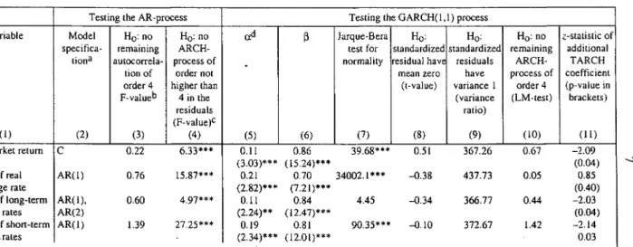
Table 2 — Testing the AR/GARCH Models for the Financial Variables

Variable

(1) Stock market return Change of real exchange rate Change of long-term interest rates Change of short-term interest, rates

Testing the AR-process Model specifica-tion3 (2) C AR(1) AR(1), AR(2) AR(1) HQ: no remaining autocorrela-tion of order 4 F-value" (3) 0.22 0.76 0.60 1.39 Ho: no ARCH-process of order not higher than 4 in the residuals (F-value)c (4) 6.33*** 15.87*** 4.97*** 27.25*** ad (5) 0.11 (3.03)*** 0.21 (2.82)*** 0.11 (2.24)** 0.19 (2.34)*** (3 (6) 0.86 (15.24)*** 0.70 (7.21)*** 0.84 (12.47)*** 0.81 (12.01)***

Testing the GARCH(1, Jarque-Bera test for normality (7) 39.68*** 34002.1*** 4.45 90.35*** Ho: standardized residual have mean zero (t-value) (8) 0.51 -0.38 -0.34 -0.10 1) process Ho: standardized residuals have variance 1 (variance ratio) (9) 367.26 437.73 366.77 372.67 Ho: no remaining ARCH-process of order 4 (LM-test) (10) 0.67 0.05 0.44 1.42 c-statistic of additional TARCH coefficient (p-value in brackets) (ID -2.09 (0.04) 0.85 (0.40) -2.03 (0.04) -2.14 0.03

aC denotes a constant, AR(p) an autoregressive process of order p. — ^Breusch/Godfrey-Test. — cLM-test. — ^The number in brackets are z-statistics for

a test whether the ARCH(cc) or ARCH(f3) coefficient are equal to zero. — *(**,***) denotes rejection of the null hypothesis at thei 1 (5, 10) percent level. Source: Own estimates.

Figure 1 — Quantile/QuantiIe(Q0-Plots of the Standardized Residuals of the GARCH(l.l) Models against the Normal Distribution

O

0-- 6 0-- 4 0-- 2 0 2 4 Real exchange rale of the DM

- 4 - 2 0 2 4 6 Short-icrm interest rale

However, normality is mostly rejected by a Jarque-Bera test as can be seen from column seven of Table 2. As the QQ-p\ols depicted in Figure 1 confirm, this is mainly due to some influential outliers. In spite of this rejection, the results can nevertheless be interpreted in a meaningful way as long the squared standard-ized residuals are at least distributed with mean zero and a standard deviation of one. Hence, we apply tests of these hypotheses. The test statistics documented in the sixth and seventh column of Table 1 do not reject the null hypotheses that the standardized residuals of the estimated models have zero mean and a vari-ance equal to unity. Moreover, a well behaved process requires that the remain-ing innovations contain no autocorrelation and no additional ARCH-effects.

Both hypotheses have been tested using standard LM-tests. It turns out that with respect to this criterion the residuals are well behaved.

Finally, we employ the statistic developed by Brock, Dechert, and Scheink-man (henceforth BDS) (1987) to test for independence of the standardized residuals obtained from the GARCH(1,1) model. This test utilizes the concept of the correlation integral (Grassberger and Procaccia 1983) which gives the probability to find two m-dimensional vectors within a certain radius to each other. The idea behind the BDS test is to compare the correlation integral ob-tained for an embedding dimension m with the correlation integral of an i.i.d. series simply computed as the correlation integral of dimension one raised to the power m. BDS show that under the null hypothesis of i.i.d. random data their statistic is asymptotically /V(0,l) distributed. In order to neatly equalize the empirical size to the nominal size of the test, we follow De Lima (1996) and take the natural logarithm of the squared standardized residuals of our GARCH models before testing for independence. Table 3 reports the results of the BDS test for various embedding dimensions m. Following the literature (cf. e.g. Hsieh 1989), the radius has been set equal to the standard deviation of the data.

The results of employing the BDS test presented in Table 3 indicate that the standardized residuals of the GARCH(1,1) model can be considered as i.i.d. The only exception is obtained in the case of the short-term interest rate when choosing an embedding dimension of two. However, the test statistic declines rapidly as the dimension of the vector space increases. Thus, the simple GARCH(1,1) model seems to capture the main characteristics of the conditional mean and conditional variance of the financial time series.

Table 3 — BDS-tests on i.i.d. Standardized Residuals of the GARCH(1,1) models Time series

Stock market return Change of real exchange rate Change of long-term interest rate Change of short-term interest rate

2 -0.91 -0.24 -0.75 2.67* Dimension 3 -0.93 0.51 -0.17 1.96 * denotes significance at the 5 percent level. Radius set to the

- 1 1 0 1 4 5 00 -0.74 19 15 42 standard deviation under investigation. See text for details. Estimates were obtained by

developed by Dechert (1988). running the 1.52 0.48 1.13 of series program

10

Though the results of the diagnostic tests suggest that the chosen specification of the conditional vaiiance equations models work well we also tested whether a more sophisticated model possibly outperforms the simple GARCH(1,1) process. In order to detect possible asymmetries, we test whether the Thresh-old-ARCH(l,l) model independently developed by Glosten, Jagannathan and Runkle (1993) and Rabenmananjara and Zakoian (1993) outperforms the GARCH(1,1) model. The specification for the conditional variance of the TARCH(U) model is:

(3) a,2 = a) + ae;_, + (3a,2, + SD^e2.,

where D, = 1 if e, < 0. The z-values of the TARCH coefficients reported in the eleventh column of Table 1 indicate that only the real exchange rate seems to be adequately modeled by a symmetric GARCH model. In spite of the statistically significant results obtained from the tests for asymmetric GARCH effects, the impact of allowing for asymmetric news impulse functions on the time series of the conditional variance turned out to be rather modest. The time series of the conditional variance computed by applying the competing GARCH specifications were found to be very close to each other. A similar proposition holds true for the news impulse functions (Figure 2). Thus, resorting to more sophisticated conditional variance equations results only in a slightly modified magnitude of the conditional variance estimates and leaves the qualitative characteristics of the variance series unaffected.

To summarize, the GARCH(1,1) model frequently employed in empirical work captures the essential features of the volatility processes very well. Nevertheless, the departure from normality of the standardized residuals visual-ized in Figure 1 suggests that it is necessary to take heteroscedasticity into ac-count when estimating the models. In the following, the quasi-maximum likeli-hood method developed by Bollerslev and Woolridge (1992) is used to accomplish this task.

11

Figure 2 — The Estimated News Impact Curves for the GARCH and TARCH Models of the Financial Variables

Slock market returns

GARCH TARCH

Short-term interest rates

1.2 1.0 0.8 - 0.60.4 -0.2 . on. \ \ \ / /

Long-term interest rates

•GARCH TARCH

Real exchange rale

-GARCH — - T A R C H -GARCH TARCH

3.3 Characterization of the Estimated Volatility Series

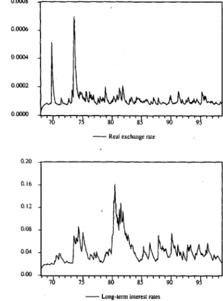
Figure 3 shows estimates of the conditional variances of our series of financial market data. All in all, the models produce economically reasonable results. The volatility of the real exchange rate is considerable lower under the Woods-System than afterwards. Not surprisingly, the end of the Bretton-Woods-System produced a sudden burst of volatility. The other peaks of the volatility series of the real exchange rate reflect realignments in the EMS sys-tem (for example 1982, 1990, 1992). The picture for the short-term interest rate volatility contrasts the result for the exchange rate. The frequency of short-term

Figure 3 — Conditional Variances of Selected Financial Variables

'70 ' ' ' 75 ' ' ' 80 ' ' ' 85 ' ' ' '96 ' ' ' '95 ' ' ' Slock market returns

J

75 80 85 90 95 Short-term interest rate

0.0008 0.0006 0.0004 0.0002 0.0000 0.20 0.16 0.12 0.08 0.04 -0.00 '76 ' ' ' '75 ' ' ' '80 ' '85 Real exchange rate

'70 ' ' ' '75 ' ' ' '86 ' ' ' '85 ' ' ' "90 ' '95 • Long-term interest rates

interest rate volatility peaks is clearly higher under the Bretton-Woods system than under a system of freely floating exchange rates or under the EMS ex-change rate target zone. Obviously, the Bundesbank had to accept more volatile short-term interest rates to stabilize the external value of the currency. In recent years, the volatility of both long- and short-term interest rates has been remark-ably low. This seems to reflect a non hectic monetary policy. Moreover, the volatility of short-term interest rates is considerably higher than the volatility of long-term rates. This in line with previous studies (cf. e.g. Sill 1993) and sounds quite reasonable since short-term rates should be seen as a political instrument. However, the gap between the two volatility measures is obviously narrowing. The graph depicting stock market volatility exhibits two pronounced peaks in 1987 and in 1991 which reflect the bearish stock market during these episodes. For example, the burst of volatility in 1987 clearly captures the magnifying im-pact of the Crash on stock market volatility. Visual inspection of the conditional variance series also suggests that stock market volatility typically decline im-mediately after crashes. Such a result has also been found by Schwert (1990).

4. Financial Market Volatility and the Business Cycle 4.1 Testing for Cyclical Patterns in Financial Market Volatility

To test whether a link between financial market volatility and real economic activity exists, one first has to define the phases characterizing the cyclical movement of the business cycle in an appropriate way. There are, in general, two ways of defining the phases of the business cycle which can be found in the literature. One idea is that a business cycle should be seen as a deviation of out-put from a trend or a potential outout-put variable. We use the filter developed by Hodrick and Prescott (1997) to measure the trend, choosing a smoothing para-meter of A = 14 400 as it is usually done for monthly data. Declines of real eco-nomic activity, that is, recessions are then defined as a negative trend deviation of more than 1.0 percent. Alternatively, we measure the time from business cycle peaks to troughs to identify phases of downswing of real economic activity. The second approach in classifying business cycle phases is to define

14 Figure 4 — Phases of West Germany's Business Cycle

Peak to Trough - Based on Trend Deviations

p.c.

p.c.

68 70 72 74 76 78 80 82 84 86 88 90 92 94 96 98 Recession Phases - Based on Trend Deviations

68 70 72 74 76 78 80 82 84 86 88 90 92 94 96 98 Recession Phases - Based on Year-on Year-Changes

p.c.

68 70 72 74 76 78 80 82 84 86 88 90 92 94 96 98 Shaded areas: Downswings and Recessions, respectively.

15

the cycle using absolute changes over the previous year. A recession period is then defined as months with a negative change of industrial production as com-pared to the year before. Applying these classification schemes, we obtain the business cycle phases depicted in Figure 3. In this figure, the shaded areas represent downswings and recessions, respectively. The large outliers in 1984 are due to a strike in the manufacturing sector.

If financial market volatility should provide information concerning the busi-ness cycle it should have a cyclical pattern itself. In order to test for potential cyclical characteristics of our volatility series, we investigate whether financial market volatility exhibits a similar behavior in recession as compared to non-recession periods. A shortcoming of this technique is that the data are grouped according to a recession/non-recession scheme which neglects valuable infor-mation potentially provided by the chronological ordering of the data. The first test is, therefore, supplemented by the computation of the autocorrelation coefficients of the volatility variables for various lag lengths.

Table 4 compares the level of conditional variances during recessions and during expansions (for similar results using U.S. data see Schwert 1989b). Overall, the results of this analysis indicate that financial market volatility is significantly higher during periods of economic downswings and recessions, respectively. There are only minor exceptions: real exchange rate and long-term interest rate volatility are not higher in or prior to recessions defined on the basis of trend deviations. This difference in the results obtained by applying the two definitions of recession might reflect the fact that, given that there is some positive trend growth, an absolute decline of industrial production will indicate a relatively strong recession, whereas the trend deviation will count more months as recession months.

These results suggest that a link between financial market volatility and the business cycle situation exists. This proposition can further be tested by examining the autocorrelation functions of the volatility series. Table 5 provides the time series autocorrelation coefficients for selected lags. As can be seen from this table, the autocorrelation functions decay slowly and are strictly positive in almost all cases. The autocorrelation functions confirm the result already obtained in Section 2 that the volatility series exhibit a remarkable degree of persistence. The results, however, do not support the notion that the

16

conditional volatility of our financial market series show any cyclical behavior which could be claimed to match the length of a typical business cycle.

Table 4 — Tests for a Similar Behavior of Financial Market Volatility in Recession as Compared to Non-recession Periods

Variable Stock market volatility Real exchange rate volatility Long-term interest rate volatility Short-term interest rate volatility *(**,***) denotes percent level. Downswing phases defined on the basis of

trend deviations t-test Mann Whitney test Recession defined on trend deviations t-test Mann Whitney test Recession defined on year on year changes

t-test Mann Whitney test 2.27** 0.35 3.07*** 2.17** 3.71*** 3.26*** 3.13*** 3.80*** 1.91* 0.73 0.75 5.66*** 7.68*** 5.80*** 1.64 0.79 9.56*** 7.56*** 4.30*** 2.82** 0.35 3.49*** 6.14*** 4.73*** that the null hypothesis of an equal mean is rejected at the 10 (5, 1)

Table 5 — Autocorrelation Coefficients of the Volatility Variables

Stock market volatility Volatility of

the real ex-change rate Volatility of long-term interest rates Volatility of short-term interest rates Pi 0.92 0.80 0.93 0.93 P2 0.82 0.57 0.87 0.83 P3 " 0.74 0.40 0.81 0.71 P4 0.66 0.29 0.75 0.61 P8 0.39 0.04 0.59 0.42 Pl2 0.20 0.05 0.49 0.34 P24 0.16 -0.00 0.06 0.14 P36 0.22 -0.02 -0.12 -0.08 Q(36) 1702.9*** 485.7*** 2557.8*** 1748.9*** Q(36) denotes a Liung-Box-Statistic for a test whether there is autocorrelation of order 36. — *** denotes a rejection at the 1 jercent level.

17

4.2 Does Financial Market Volatlity Send the Right Signal?

In order to analyze the properties of the conditional variances of our financial market variables as potential leading indicators of the business cycle in more detail, we now use the signal approach as outlined for example in Kaminsky and Reinhard (1998). This method works as follows (see also Schnatz 1998).

Assume that an appropriate variable has been detected which is suspected to provide some information regarding the value of coming realizations of another series or the subsequent occurence of a certain event. Say this indicator gives a "signal" and it turns out to be correct and denote this case with an A. A false signal is denoted by a B. If the indicator gives no signal and this turns out to be correct symbolize this event by a D. Finally, the letter C represents the case that the indicator does not send a signal but an event takes place. Given these defini-tions, it is possible to compute the following numbers:

- The share of correct signals compared to the number of all signals: (A/(A+C)).

- The noise-to-signal ratio given by (B/(B+D) I A/(A+C)). This number should

be as small as possible since the indicator should give in the best case no false signals. For a pure random forecasting process the expected value of this ratio is 1.

- The odds-ratio definded as (A*D)/(B*C). If the forecast is purely random, there will be as many correct as false signals, i.e. the odds-ratio will be equal to one. If it exceeds one, the probability of receiving a correct signal is larger than the probability of receiving a false signal.

In the context of the present analysis, the indicator variables are the estimated conditional variances of the financial time series. The events which are to be predicted correctly are slowdowns of economic activity. A realization of finan-cial market volatility is counted as a "signal" of a future slowdown of real economic activity if it exceeds its median computed for the entire sample period. In order to give the conditional financial market volatility series a fair chance to send a right signal, a warning is counted as a correct information if an "event", i.e. a downswing or a recession, respectively, indeed takes place within a period of twelve months after the financial market volatility has sent the sig-nal.

Having already constructed time series describing the phases of the business cycle, we are now in a position to apply the signal approach to check the

fore-18

casting properties of financial market volatility. Table 6 reports the results of this:exercise. The numbers plotted in Table 6 show that in almost all cases the

financial market volatility series provide only very limited information about the coming business cycle situation. Comparing the results obtained for the different measures of real economic activity, it can further be seen that the forecasting power of the volatility series critically depends upon the measure of real economic activity used in the analysis. For example, the noise to signal and the odds ratio obtained for the volatility of the real exchange rate indicate a significant informational content of this indicator if real economic activity is classified utilizing downswings defined on the basis of trend deviations. In contrast, if one uses negative trend deviations of more than 1.0 percent to identify recessions the quality of a signal sent by the volatility of the real ex-change rate does not exceed the quality of a signal received from a purely random variable. As regards short-term and long-term interest rate volatility, the forecasting power of these indicators reaches a maximum if a recession is defined on the basis of year-to-year changes. The quality of these indicator variables is, however, poor if the other two measures of the business cycle are used to compute the noise to signal and the odds ratio. Computing these ratios for stock market volatility indicates that the signals sent from this measure of financial market volatility do not provide reliable information for all measures of the business cycle. This result, thus, confirms Samuelson's remark that "The stock market has predicted nine out of the last five recessions." (Samuelson 1966).

In a nutshell, the results obtained by applying the signal approach suggest that our measures of financial market volatility almost always do not send reliable signals regarding subsequent changes of real economic activity. However, Table 6 also indicates that the forecasting power of the volatility series might depend upon the classification scheme utilized to measure the stance of the business cycle. This finding suggests that it is necessary to apply more formal techniques to test for the link between financial market volatility and the business cycle.

Table 6 — "Noise to Signal" and "Odds"-Ratio for the Volatility as a Leading Indicator for the Output Gap

Variable

Stock market volatility Real exchange rate

volatility Long-term interest

rate volatility Short-term interest

rate volatility

Downswings defined on the basis of trend deviations Number of correct signals 0.45 0.59 0.53 0.50 Noise to signal ratio 1.34 0.55 0.86 0.99 Odds ratio 0.55 2.97 1.35 1.02

Recession defined on the basis of trend deviation Number of correct signals 0.55 0.53 0.53 0.55 Noise to signal ratio 0.83 0.90 0.88 0.83 Odds ratio 1.47 1.23 1.29 1.47

Recession defined on year on year

Number of correct signals 0.50 0.59 0.66 0.56 changes Noise to signal ratio 1.01 0.68 0.51 0.79 Odds ratio 0.99 2.18 3.81 1.60 Source: Own calculations.

20

4.3 Testing for Causality Patterns

In this section we utilize alternative methodologies to elaborate on the possible link between the volatility of financial variables and real economic activity. In addition to an analysis of the relation between the level of real activity and financial market volatility measures as already performed in the preceding sections we now also examine whether the financial market series and the business cycle measures are linked through the conditional second moments. We, thus, test the hypothesis that real volatility and financial market volatility are interrelated.

An oftenly used statistical technique in the business cycle literature to test for the predictive power of an economic variable with respect to future changes of the level real economic activity is the test for Granger-non-causality. Let the (stationary) time series measuring the business cycle be denoted by Y,. Then the following bivariate autoregressive representation is estimated:

(4)

The lag length s is chosen using the minimum Schwartz-information-criterion. Then, the hypothesis that the conditional variance does not Granger cause the output gap (i.e. (3, = 0) can be tested performing a standard F-test. It will also be analyzed whether the output gap does not Granger-cause volatility (i.e.

<5, =0). If both hypothesis cannot be rejected it is a feedback relationship. Table 7 gives the results of this testing procedure. It turns out that none of the financial variable volatility measures Granger-causes the level of the business cycle variable. The reverse relationship only occurs in the case of the volatility of long-term interest rates. Hence, the volatility of the series under investiga-tion provides no predictive power for the business cycle as measured by the level of industrial production.

21

Table 7 — Testing for Granger-non-causality with Respect to the Output Gap Time Series Stock market volatility Volatility of real exchange rate Long-term interest rate volatility Short-term interest rate volatility Lag-length of VAR 2 2 2 2 Schwartz criteria -8.33 -13.67 -3.01 1.52 Ho: Volatility does not Granger cause real 0.08 0.04 1.15 0.39 Ho: Real economic activity does not Granger cause the volatility 0.15 1.14 4.02** 0.02 Decision no causality no causality gap causes volatility no causality

Since the volatility series exhibit some strong peaks, one might ask whether the VAR's used to estimate the Granger-non-causality are stable over time. There are indeed several points in time at which a structural break might have taken place. For example, the influence of real exchange rate (volatility) could have changed after the breakdown of the Bretton-Woods system. The same might hold true for the volatility of the short-term interest rates since they are much more volatile under the fixed exchange rate system than afterwards. Moreover, there has been a substantial change in the direction of monetary policy in the eighties as compared to the seventies. To test for possible structural breaks reducing the power of the Granger-non-causality tests we apply a simple recursive procedure outlined in Bianchi (1995). Basically, a dummy variable is added to the two equations of the VAR which assumes the value 0 before a breakpoint and 1 afterwards. Then, beginning at January 1970, the possible breakpoint is moved forward in time and the VAR are estimated recursively. Figure 5 depicts the marginal probabilities of the resulting tests on Granger-non-causality for the output gap. As can be read off Figure 5, the results of the tests are fairly stable.

Figure 5 — Recursive Tests on Granger-non-causality Stock market return

I BO: yplaulHV does not wanner-cause cycle .. i HO: Cycle does not granger-cause volatility

10 percent level

76 78 80 82 84 86 90 92 94 96

Short term interest rate

HO: Volatility docs not granger-cause cycle

HO: Cycle does not granger-cause volatility

10 percent level

76 78 80 82 84 90 92 94 96 98

Real exchange rate

0.6

0.4

0.2

0.0 -\

HO: Volatility docs not granger-cause cycle

HO: Cycle does not granger-cause volatility

10 percent level

76 78 80 82 84 86 92 94 96

Long-term interest rate

0.6 0.5 0.4 0.3 0.2 -0.1 0.0

HO: Volatility docs not granger-cause cycle

10 percent level

HO: Cycle does not granger-cause volatility

76 78. 80 82 84 90 92 94 96 98

to to

23

It is also interesting to examine whether the relation between financial market volatility and the business cycle is asymmetric. For example, high stock market volatility combined with falling stock prices might exert another impact on the level of real economic activity than high volatility in times of a rising stock market. Thus, the reaction of the level of real economic activity to financial market volatility might depend on the sign of the change of the financial time series. To test this hypothesis, we reestimate the equations forming the VAR using dummy variables constructed in a way to capture the sign of a change of the financial market series (see Table 8). We then perform exclusion tests to study for the explanatory power of the dummies (Huh 1998). The tests are built on the following augmented equations:

Y.'= ao + 0 • dummy, + s ( a , + Q* dummy )Y .

(5)

af =yo + ©dummy, + s(y, + ®fdummy,)a,2_,

0fdummy,)]^_( + e2(

•u

The results of this exercise are reported in Table 8. In general, the hypothesis that the dummy is not significantly different from zero cannot be rejected. Thus,

Table 8 — Dummy Variable Exclusion Test on Stability of the Granger-non-causality Tests Dummy

1 if stock-market return <0, 0 else 1 if change of real exchange rate <0,

Oelse

1 if change of long-term interest rate <0, 0 else

1 if change of short-term interest rate is 1,0 else

F-statistic; p-value in brackets.

Ho: Dummies not

different from zero in equation for gap

Ho: Dummies not

different from zero in equation for volatility 0.59 (0.77) 0.79 (0.60) 2.32 (0.04) 9.41 (0.00) 1.62 (0.16) 0.12 (0.99) 0.62 (0.66) 1.84 (0.11)

24

taking asymmetries into account does not alter the conclusions drawn from the tests for Granger-non-causality. The only exception obtains in the case of real exchange rate volatility. The result of the dummy variable exclusion test indi-cates that the sign of real exchange rate changes should be taken into con-sideration when examining the impact of real exchange rate volatility on the level of real economic activity.

To summarize, the tests for Granger-non-causality confirm the results pro-duced by applying the signal approach. The results of these test procedures sug-gest that financial market volatility has only a very limited -if any- predictive power with respect to subsequent changes of real economic activity. This finding, of course, does not imply that the level of important financial variables is of no relevance for the evolution of the real sector. However, our results indicate contrary to often made assumptions that financial market turbulences do not exert a significant impact on the business cycle.

Another question is whether there is a causal relationship between the volatility of the financial variables and the volatility of industrial production (see also Kearney and Daly 1997). To investigate this, an ARCH(l) model is specified for the index of industrial production as well. To take into account the strike in the manufacturing sector, a dummy variable is added to the AR-process for IP which takes the value - 1 in 1984:06 and 1 in 1984:07.

The following results were obtained:

A\n IP, = 0.002 - 0.304 A In IP . + 0.095 A In IP . - 0.089 STRIKE + e,

(2.73) (-6.49) (2.28) (-22.9) '

Q>\ = 0.0002 + 0.223 ef,

(9.09) (2.57)

R2: 0.29; Jarque/Bera test for normality = 10.52; ARCH LM(4) = 1.39;

stan-dardized residual mean equal to zero -0.58; stanstan-dardized residuals have standard deviation of one 336.98 BDS-test on i.i.d. (dimension = 2, radius set equal to standard deviation of squared logarithms standardized residuals): 0.29, BDS(3): 0.38, BDS(4): 0.19.

We are now in a position to perform causality-in-variance tests as suggested by Cheung and Ng (1996). The test statistics utilize the cross-correlation function of squared standardized residuals to identify possible links between the second moments of two series. Let fxp{k) denote the sample cross-correlation

25

at lag k of the squared standardized residuals obtained from the (G)ARCH models specified for the financial market series x and industrial production. Premultiplying r(k) with the square root of the number of observations yields a statistic which is N(0.1) distributed under the null of non-causality in volatility at lag k. Alternatively, Cheung and Ng propose a chi-square test statistic to examine the null hypothesis of no causality from lag j to lag k:

%l_M = T • Zf=y rx,P(}f ' where T symbolizes the number of observations and the

salar (k — j + 1) denotes the degrees of freedom. Table 9 — Tests on Causality-in-variance

Ho: Stock market

volatility does not cause real volatility Ho: Real volatility does

not cause stock-market volatility Ho: Exchange rate volatility does not cause real volatility Ho: Real volatility does

not cause exchange rate volatility Ho: Long-term interest

rate volatility does not cause real volatility Ho: Real volatility does

not cause long-term interest rate volatility Ho: Short-term interest

rate volatility does not cause real volatility Ho: Real volatility does

not cause short-term interest rate volatility

1 -0.79 0.59 0.61 -0.30 -0.21 0.01 0.21 0.10 2 -1.30 -0.03 1.40 1.38 -0.44 -1.47 -0.16 -0.72

1 ^

All lags 9.85 10.68 8.18 6.09 10.77 6.91 14.05 8.05

Table 9 depicts the results of these tests. The numbers presented in the table show that there is no causality-in-variance in either direction. Neither the t-test

26

for causality at individual lags nor the chi-squared for all lags lead to a rejection of the null hypothesis of no causality in second moments. These results confirm the result of the Granger-causality tests.

5. Conclusion

This paper has used monthly data for Germany to elaborate on the possible link between financial market volatility and real economic activity. The findings of our empirical analyses spanning the period 1968 to 1998 strongly indicate that the hypothesis that the conditional variance obtained for various important financial market variables do not predict changes of real economic activity can-not be rejected.

Our result that the business cycle is not driven by the volatility of interest rates are in line with previous estimates of Schwert (1989a) for American data. This suggests that it is the level of these financial variables which is important for real economic activity rather than the volatility.

However, our insignificant estimates regarding the impact of real exchange rate and of stock market volatility on the business cycle are in contrast to results documented in related studies. As noted in the introduction, Schwert (1989) as well as Liljblom and Stenius (1997) find that stock market volatility Granger-causes the American and the Finnish business cycle, respectively. Moreover, Bell and Campa (1997), Campa and Goldberg (1995), and Mailand (1998) present evidence that the real sector of the economy is negatively affected by volatile exchange rates.

There might be several reasons for these conflicting results. With respect to the stock market, some of the studies finding significant results span an obser-vation period which includes the Great Crash of 1929. Following Romer (1990), it would thus be possible to claim that during the period covered by our sample period stock market volatility has just not been significant and enduring enough to exhibit a noticeable impact on real economic activity.

Moreover, fluctuations in financial markets might represent to some extent the influence of speculative noise trading and might, thus, be hot entirely related

27

to economic fundamentals. Such an interpretation would be in line with the findings of e.g. Flood and Rose (1995) for exchange rates.

It might also be a promising approach to highlight a potential link between uncertainty and real economic activity to resort to data on the firm level. For example, Leahy and Whited (1996) use panel date for the US and indeed find a link between stock market volatility and firm's investment decisions. In view of this evidence, it would be rather hasty to interprete our empirical results as a falsification of theories emphasizing the importance of uncertainty for invest-ment and consumption decisions.

Finally, our study has been exclusively concerned with the impact of financial market volatility on real economic activtiy. Using measures designed to capture uncertainty regarding the unpredictable future evolution of real economic vari-ables like wages and other cost determinants (Seppelfricke 1996), demand, or political factors it might be possible to empirically document a closer link between volatilty and the business cycle.

Thus, there is ample room for further research on the relevance of uncertainty for real economic activity. However, our empirical analysis in any case suggests that it might be rather fruitless to utilize financial market volalitity as a leading indicator of the business cycle.

28

Appendix Table 1 — Unit Root Test for the Variables under Investigation Time Series

Stock market index, level Real exchange rate, level Long-term interest rate, level Short-term interest rate, level Industrial production, level Stock market index, first

difference

Real exchange rate, first difference

Long-term interest rate, first difference

Short-term interest rate, first difference

Industrial production, first difference Test specification Ct,0 Ct, 1 C 2 C 1 C, t, 1 CO CO C 1 CO

c,o

29

Appendix Figure 1 —Quantile/QuantiIe(QQ)-Plot of the Standardized Residuals of the ARCH(1,1) Model for Industrial Production against the Normal Distri-bution

•"3

9

O

Industrial Production

30

References

Bell, G.K., and J. Campa (1997). Irreversible Investment and Volatile Markets: A Study of the Chemical Processing Industry. The Review of Economics and

Statistics 79: 79-87.

Bernanke, B. (1983). Irreversibility, Uncertainty, and Cyclical Investment.

Quarterly Journal of Economics 98: 85-106.

Bianchi, M. (1995). Granger Causality in the Presence of Structural Changes. Discussion Paper No. 33. Bank of England.

Bollerslev, T. (1986). A Generalized Autoregressive Conditional Hetero-scedasticity. Journal of Econometrics 31: 307-327.

Bollerslev, T., and J.M. Woolridge (1992). Quasi-Maximum Likelihood Esti-mation and Inference in Dynamic Models with Time-varying Co variances.

Econometric Reviews 11: 143-179.

Brock, W.A., D.W. Dechert, and J.A. Scheinkman (1987). A Test of Indepen-dence Based on the Correlation Dimension. SSSRi Working Paper no. 8702, Department of Economics. University of Wisconsin-Madison.

Caballero, R.J. (1992). Durable Goods: An explanation for their Slow Adjust-ment. Journal of Political Economy 101: 351-364.

Campa, J., and L.S. Goldberg (1995). Investment in Manufacturing, Exchange-Rates, and External Exposure. Journal of International Economics 38: 297-320.

Cheung, J.W., and L.K. Ng (1996). A Causality-in-variance Test and its Application to Financial Market Prices. Journal of Econometrics 72: 33-48. Dechert, D.W. (1988). BDS-STATS Version 8.21.

De Lima, P.J.F. (1996). Nuisance Parameter Free Properties of Correlation Integral Based Statistics. Econometric Reviews 15: 237-259.

Deutsche Bundesbank (various issues). Monthly Reports. Frankfurt am Main. Dixit, A.K. (1989). Hysteresis, Import Penetration, and Exchange Rate

Pass-Through. Quarterly Journal of Economics 104: 205-228.

Dixit, A.K. (1992). Investment and Hysteresis. Journal of Economic

31

Dixit, A.K., and R.S. Pindyck (1994). Investment under Uncertainty. Princeton, NY.

Engle, R.F. (1982). Autoregressive Conditional Heteroscedasticity with Esti-mates of the Variance of U.K. Inflation. Econometrica 50: 987-1008. Episcopos, A. (1995). Evidence on the Relationship between Uncertainty and

Irreversible Investment. The Quarterly Review of Economics and Finance 35: 41-52.

Federer, J.P. (1993). The Impact of Uncertainty on Aggregate Investment Spending: An Empirical Analysis. Journal of Money, Credit, and Banking 25: 3 0 ^ 8 .

Flood, R.P., and A.K. Rose (1995). Fixing Exchange Rates — A Virtual Quest for Fundamentals. Journal of Monetary Economics 36: 3-37.

Glosten, L.R., R. Jagannathan and D. Runkle (1993). On the Relationship between the Expected Value and the Volatility of the Nominal Excess Return on Stocks. Research Department Staff Report no. 157, Federal Reserve Board of Minneapolis.

Grassberger, P., and I. Procaccia (1983). Measuring the Strangeness of Strange Attractors. Physica 9D: 189-208.

Hassler, J. (1993). Effects of Variations in Risk on Aggregate Demand — The Empirics. Seminar paper no. 554, Institute for International Economics, Stockholm University, Stockholm.

Hodrick, R.J., and E.C. Prescott (1997). Postwar U.S. Business Cycles: An Empirical Investigation. Journal of Money, Credit and Banking 29: 1-16. Hsieh, D.A. (1989). Testing for Nonlinear Dependence in Daily Foreign

Ex-change Rates. Journal of Business 62: 339-368.

Huh, C. (1998). Forecasting Industrial Production Using Models With Business Cycle Asymmetry. Federal Reserve Bank of San Francisco. Economic

Review 1:29-41.

Ingersoll, J.E., and S.A. Ross (1988). Waiting to Invest: Investment and Uncertainty. Journal of Business 50: 1-29.

32

Kaminsky, G., and CM. Reinhart (1998). Financial Crises in Asia and Latin America: Then and Now. American Economic Review, Papers and

Proceed-ings 88: 444-448.

Kearney, C , and K. Daly (1997). Monetary Volatility and Real Output Volatili-ty: An Empirical Model of the Financial Transmission Mechanism in Australia. International Review of Financial Analysis 6: 77-95.

Leahy, J.V., and T.M. Whited (1996). The Effect of Uncertainty on Investment: Some Stylized Facts. Journal of Money, Credit, and Banking 28: 64-83. Liljeblom, E., and M. Stenius (1997). Macroeconomic Volatility and Stock

Market Volatility: Empirical Evidence on Finnish Data. Applied Financial

Economics 7: 419—426.

Mailand, W. (1998). Zum EinfluB von Unsicherheit auf die gesamtwirtschaft-liche Investitionstatigkeit. HWWA-Diskussionspapier Nr. 57. Hamburg. Mirman, L. (1971). Uncertainty and Optimal Consumption Decisions.

Econo-metrica 39: 179-185.

Pagan A.R., and G.W. Schwert (1990). Alternative Models of Conditional Stock Volatility. Journal of Econometrics 45: 267-290.

Pindyck, R.S. (1991). Irreversibility, Uncertainty, and Investment. Journal of

Economic Literature 29: 1110-1148.

Rabenmananjara, R., and J.M. Zakoian (1993). Threshold ARCH Models and Asymmetries in Volatility. Journal of Applied Econometrics 8: 31—49. Romer, CD. (1990). The Great Crash and the Onset of the Great Depression.

Quarterly Journal of Economics 105: 597-624.

Samuelson, P. (1966). Science and Stocks. Newsweek, September 19: 92. Scheide, J., and R. Solveen (1998). Should the European Central Bank Worry

about Exchange Rates? Konjunkturpolitik 44: 31-51.

Schnatz, B. (1998). Macroeconomic Determinants of Currency Turbulences in Emerging Markets. Discussion Paper of the economic research group of the Deutsche Bundesbank No. 3/98. Frankfurt am Main.

Schwert, G.W. (1989a). Why does Stock Market Volatility Change over Time?

33

Schwert, G.W. (1989b). Business Cycles, Financial Crises, and Stock Volatili-ty. Carnegie-Rochester Conference Series on Public Policy 31: 83-126. Schwert, G.W. (1990). Stock Volatility and the Crash of '87. The Review of

Financial Studies 3: 7-102.

Sercu, P. (1992). Exchange Rates, Exposure, and the Option to Trade. Journal

of International Money and Finance 11: 579-593.

Seppelfricke, P. (1996). lnvestitionen unter Unsicherheit: eine theoretische und

empirische Untersuchung fur die Bundesrepublik Deutschland. Frankfurt

am Main.

Sill, D.K. (1993). Predicting Stock Market Volatility. Business Review Federal