Durham Research Online
Deposited in DRO: 10 August 2016
Version of attached le: Accepted Version
Peer-review status of attached le: Peer-reviewed
Citation for published item:
Han, C. and Taamouti, A. (2017) 'Partial structural break identication.', Oxford bulletin of economics and statistics., 79 (2). pp. 145-164.
Further information on publisher's website: https://doi.org/10.1111/obes.12153
Publisher's copyright statement:
This is the accepted version of the following article: Han, C. Taamouti, A. (2017). Partial Structural Break
Identication. Oxford Bulletin of Economics and Statistics, 79(2): 145-162, which has been published in nal form at https://doi.org/10.1111/obes.12153. This article may be used for non-commercial purposes in accordance With Wiley Terms and Conditions for self-archiving.
Additional information:
Use policy
The full-text may be used and/or reproduced, and given to third parties in any format or medium, without prior permission or charge, for personal research or study, educational, or not-for-prot purposes provided that:
• a full bibliographic reference is made to the original source
• alinkis made to the metadata record in DRO
• the full-text is not changed in any way
The full-text must not be sold in any format or medium without the formal permission of the copyright holders. Please consult thefull DRO policyfor further details.
Durham University Library, Stockton Road, Durham DH1 3LY, United Kingdom Tel : +44 (0)191 334 3042 | Fax : +44 (0)191 334 2971
Partial Structural Break Identification
∗Chulwoo Han†
Durham University Business School
Abderrahim Taamouti‡ Durham University Business School July 2, 2016
ABSTRACT
We propose an extension of the existing information criterion-based structural break identification ap-proaches. The extended approach helps identify bothpure structural change (break) and partial structural change (break). A pure structural change refers to the case when breaks occur simultaneously in all pa-rameters of regression equation, whereas a partial structural change happens when breaks occur in some parameters only. Our approach consistently outperforms other well known approaches. We also extend the simulation studies of Bai and Perron (2006) and Hall et al. (2013) by including more general cases. This provides more comprehensive results and reveals the cases where the existing identification approaches lose power, which should be kept in mind when applying them.
Keywords: Identification of structural breaks, partial structural change, pure structural change, informa-tion criterion, Monte Carlo simulainforma-tion.
Journal of Economic Literature classification: C01, C1, C51, C52.
∗The authors thank the anonymous referee and the Editor Prof. Anindya Banerjee for several useful comments.
†Durham University Business School. Address: Mill Hill Lane, Durham, DH1 3LB, UK. TEL: +44 1913345892 E-mail:
‡Durham University Business School. Address: Mill Hill Lane, Durham, DH1 3LB, UK. TEL: +44 1913345423 E-mail:
Partial Structural Break Identification
ABSTRACT
We propose an extension of the existing information criterion-based structural break identification ap-proaches. The extended approach helps identify bothpure structural change (break) and partial structural change (break). A pure structural change refers to the case when breaks occur simultaneously in all pa-rameters of regression equation, whereas a partial structural change happens when breaks occur in some parameters only. Our approach consistently outperforms other well known approaches. We also extend the simulation studies of Bai and Perron (2006) and Hall et al. (2013) by including more general cases. This provides more comprehensive results and reveals the cases where the existing identification approaches lose power, which should be kept in mind when applying them.
Keywords: Identification of structural breaks, partial structural change, pure structural change, informa-tion criterion, Monte Carlo simulainforma-tion.
1
Introduction
Structural breaks have been observed in many economic and financial time series, see Stock and Watson (1996) among others. It is well established that ignoring these breaks has undesirable consequences on time series analysis. In particular, authors such as Clements and Hendry (1998, 1999) consider the ignorance of structural breaks as a main reason of forecast failure. Hence the importance of providing robust statistical procedure for detecting and estimating the number of breaks cannot be overemphasized.
Several approaches have been proposed to detect structural breaks in economic and financial time series. Andrews (1993) and Bai and Perron (1998) introduced statistical testing procedures to investigate the presence and timing of change when one or more breaks occur within the available time series data. Perron and Qu (2006) extended these results to the case where arbitrary linear restrictions on the coefficients are available a priori. Another class of approaches are based on information criteria. Yao (1988), Liu et al. (1997), and Zhang and Siegmund (2007) considered Bayesian information criterion (BIC) of Schwarz (1978), whereas Ninomiya (2005) used Akaike’s information criterion (AIC) of Akaike (1973). In addition, Bai (2000) established conditions under which an information criterion is consistent for estimation of the number of breaks in vector autoregressions with martingale difference sequence errors. Finally, recently Chen, Gerlach, and Liu (2011) have used a Bayesian computational method to identify the locations of structural breaks in the context of time-varying regression model and in the presence of heteroskedasticity and autocorrelation. In this paper, we extend the existing information criterion-based approaches to identify both pure and partial structural changes. A pure structural change refers to the case when breaks occur simultaneously in all parameters of regression equation, whereas a partial structural change refers to the case when breaks occur in some parameters only. One drawback of the existing approaches is that they assume pure (simultaneous) structural breaks only, although this may not be the case in reality. For example, if a monetary policy measure is included as one of the regressors and one wants to examine the effect of changes in this measure on a dependent macro variable, there is no reason to assume that other regressors will also experience a structural break at the same time. If breaks occur only in some of the regressors, as explained in Section 3, the existing information criterion-based approaches will underestimate the number of breaks. Our extension aims to address this problem of the existing approaches and detect partial structural breaks as well as pure structural breaks.
Another contribution of this paper is that we provide a Monte Carlo simulation study which compares the performance of our approach with the exiting ones for a large set of data-generating processes that represent different contexts encountered in practice. We extend the simulation studies of Bai and Perron (2006) and Hall et al. (2013) by including more general cases, especially the cases where break detection becomes difficult. This provides more comprehensive results and reveals the potential areas where the
existing methods lose their power. Simulation results show that our approach consistently outperforms other well known approaches such as the ones introduced by Yao (1988) and Bai and Perron (1998).
The rest of the paper is organized as follows. The framework that defines the regression model with multiple breaks and a general procedure that identifies these breaks is introduced in Section 2. Section 3 provides a brief summary of the existing information criterion-based approaches and discusses our approach for detecting partial breaks. In Section 4, we use Monte Carlo simulations to investigate the performance of our approach by comparing it with the existing ones. Section 5 concludes.
2
Framework
We consider the followingN-variable linear system with K breaks
yt=Xtβk+et, for τk−1 ≤t < τk, with k= 1,· · ·, K+ 1, (1)
whereXt= [1x1t · · · xN t] is a vector of covariates, βk= [β0k · · · βN k]′ is a vector of parameters of interest
that are subject to multiple structural breaks, and et is an error term. K breaks means that we are in presence ofK+ 1 regimes that are defined by the time set{τ0= 1, ..., τK+1=T}within the whole sample of
sizeT. The problem now is to identify the number (K) and timing (τk) of the breaks. A general procedure for this consists of the following two steps:
Identification of the timing of breaks: The first step is to findτk,fork= 1,· · · , K,that minimize the
residual sum of squares (RSS). Formally, we selectτ1,· · · , τK that minimize the RSS:
{τˆ1,· · · ,τKˆ }= argmin τ1,···,τK { RSSK = K∑+1 k=1 RSSk } , (2) where RSSk= τk ∑ t=τk−1+1 (yt−Xtβkˆ )2, fork= 1,· · ·, K+ 1. (3) This is repeated for K = 0,· · · , Kmax, a pre-specified maximum number of breaks. As noted by Bai and
Perron (2006), there areT(T−1)/2 possible regimes within the sample.1 Therefore, the global minimum of the problem in (2) can be found efficiently as follows: 1) calculateRSSk for all the possible regimes; 2) for
a given set ofτ1,· · ·, τK, choose the correspondingRSSk’s and simply add them up to obtain RSS. Determination of the number of breaks: The second step is to determine the number of breaks by comparing the global minima forK = 1,· · ·, Kmax. This normally consists of using a statistical test-based procedure such as the one in Bai and Perron (1998, 2003, 2006) and Perron and Qu (2006) or an information criterion-based approach as in Yao (1988), among others.
1
3
Information criterion-based approaches
3.1 Brief summary of the existing approaches
Several information criterion-based identification methods have been proposed to determine the number of breaks. The first and well known approach was introduced by Yao (1988). He shows that when the residuals
et in (1) are i.i.d. normal, breaks in mean can be identified using the Bayesian information criteria (BIC) of
the form:
BIC(K) =TlogRSSK
T + ((N+ 1)(K+ 1) +K) logT, (4)
whereRSSK is the residual sum of squares at its minimum as defined in (2),N is the number of covariates
in the regression equation (1),K is the number of breaks, and T is the sample size. Yao (1988) suggests to choose the number of breaksK that has the minimum BIC, i.e.,
ˆ
K = argmin
K
BIC(K). (5)
Liu, Wu and Zidek (1997) have also used a BIC for the identification of number of breaks. Their approach, however, appears to underperform in the simulation analyses reported in Bai and Perron (2006) and Hall et al. (2013), and will not be considered further in this paper.
More recently, Hall et al. (2013) proposed an alternative approach where the penalty for the breaks is 3K instead ofK. Their information criteria has the form:
BIC(K) =TlogRSSK
T + ((N+ 1)(K+ 1) + 3K) logT. (6)
With the penalty term 3K, their approach is more conservative and is likely to underestimate the number of breaks compared to Yao (1988) approach.
Finally, Bai and Perron (1998, 2003, 2006) proposed sequential statistical procedures to determine the number of breaks. Perron and Qu (2006) have extended these results to the case where arbitrary linear restrictions on the coefficients are available a priori. For more details about these statistical procedures, the reader is referred to Bai and Perron (1998, 2003, 2006) and Perron and Qu (2006) or Hall et al. (2013) for a summary.
3.2 Extended approach
One drawback of Yao (1988) and other existing approaches is that they assume pure structural changes in all the regressors. However, this is not necessarily the case in many circumstances. For example, if a monetary policy measure is included as one of the regressors and we want to examine the effect of changes in this measure on a dependent variable, there is no reason to assume that other regressors will experience structural breaks at the same time. If a break occurs only in some of the regressors, as illustrated in the
following example, the term (K+ 1)(N + 1) in (4) and (6) will impose too severe penalty, and therefore it will result in underestimation of the number of breaks in finite samples.
Our extension of the existing approaches aims to address this issue by taking partial breaks into account. Note that the BIC formula in (4) can be viewed as the BIC of a dummy variable regression equation with unknownK breaks. For example, consider a bivariate system with one break at timeτ1. A corresponding
dummy variable regression equation will have the form y1 .. . yτ1 yτ1+1 .. . yT = 1 x1 1 x1 .. . ... ... ... 1 xτ1 1 xτ1 1 xτ1+1 0 0 .. . ... ... ... 1 xT 0 0 β0 β1 β2 β3 + e1 .. . eτ1 eτ1+1 .. . eT .
The BIC of this regression is the same as the one in (4). Now, if the break occurs only inx, a corresponding dummy variable regression equation will have the form
y1 .. . yτ1 yτ1+1 .. . yT = 1 x1 x1 .. . ... ... 1 xτ1 xτ1 1 xτ1+1 0 .. . ... ... 1 xT 0 β0 β1 β2 + e1 .. . eτ1 eτ1+1 .. . eT .
In this case, the correct BIC is given by:
BIC(K) =TlogRSSK
T + (N+ 1 +N K+K) logT,
whereRSSK is the residual sum of squares from the above dummy variable regression equation. Similarly, we can construct a dummy variable regression for a break in the intercept only and obtain the corresponding BIC. In general, for a system ofN + 1 regressors including constant, there areCjN+1 possible combinations of partial breaks in j regressors out of N + 1 regressors. Therefore, the total number of potential partial breaks becomes2
D=C1N+1+· · ·+CNN+1+1.
The BIC of cased, d= 1,· · · , D, can be calculated using the following formula
BIC(K, d) =TlogRSSK(d)
T + (N + 1 +nK+K) logT (7)
2
wheren and RSSK(d) are respectively the number of regressors experiencing breaks and the residual sum of squares of the corresponding dummy variable regression in cased.3 The number of breaks is determined by choosingK that minimizes the BIC in all cases. That is:
ˆ
K= argmin
K
BIC(K, d), ford= 1,· · ·, D. (8) When onlyn < N regressors experience breaks, it is sensible to adjust the penalty term proportionately to the ration/N. In this case, Equation (7) needs to be modified as follows:
BIC(K, d) =TlogRSSK(d) T + ( N + 1 +nK+ n NK ) logT. (9)
The following proposition establishes the consistency of the estimation of the number of breaksK based on the minimization problem defined in (8), whereBIC(K, d) is given by (7) or (9). The assumptions needed to derive Proposition (1) are similar to the ones considered in Yao (1988) and Liu, Wu and Zidek (1997); see for example Assumptions 4.1-4.1′ in Liu, Wu and Zidek (1997).
Proposition 1 Assume that K0 ≤Kmax, βk0 ̸=βk0+1 for 1≤k≤K0, with superscript 0 denoting the true parameters, andτk/T for 1≤k≤K0 converges toλk as T → ∞ for some 0< λ1 <· · ·< λK0 <1. Then,
Pr ( ˆ K =K0 ) →1 as T → ∞.
See Appendix A for proof. Proposition 1 is valid for both the BIC in Equation (7) or its modified version in Equation (9).
We also consider Hannan & Quinn criterion (HQC) of the form
HQC(K) =TlogRSSK
T + 2((N+ 1)(K+ 1) +K) log(logT), (10)
and its extensions.4 As 2 log(logT) < logT for T > 2, HQC based approaches are expected to overfit compared to BIC based approaches.
Through various simulations, we observe that information criterion-based methods often select zero break when the true number of breaks is greater than zero. Furthermore, in many cases, we find that the BIC of the true number of breaks,K, is often a local minimum, i.e.,
BIC(K)<min(BIC(K+ 1), BIC(K−1)).
Based on this observation, we further improve our approach by adding the following procedure (henceforth, referred to as the modification):
3Equation (7) is an extension of Yao’s (1988) model. Hall et al. (2013) model can also be extended in the same manner by
replacingKin the last term of equation (7) with 3K.
4
1. FindK’s such that
BIC(K)<min(BIC(K+ 1), BIC(K−1)), K >0.
2. If there exist at least oneK that satisfy the above condition, chooseK that has the minimum BIC as the number of breaks.
3. Otherwise, set the number of breaks to zero.
4
Monte Carlo simulation
In this section, we use Monte Carlo simulation to compare the performance of our approaches and the existing ones for various data generating processes (DGPs) that represent different contexts encountered in practice. Our DGPs are based on those of Hall et al. (2013) and Bai and Perron (2006), but we consider additional DGPs that extend the previous ones to highlight more general cases where identification approaches could lose power. We compare 12 approaches: 8 extensions and 4 existing models, as listed in Table 1. 10% trimming value is used in all models, and 10% statistical significance level is applied for Bai and Perron (2006) approaches.
Table 1: Comparison Models
Model Description
B1 Yao (1988)
B1A Extension of Yao (1998): Partial breaks (BIC defined in (7)) B1B B1A with the modification
B1C Extension of Yao (1998): Partial breaks and fractional penalty (BIC defined in (9))
B1D B1C with the modification B3 Hall et al. (2013)
B3A Extension of Hall et al. (2013): Partial breaks HQ HQC defined in (10)
HQA Extension of HQC: Partial breaks HQB HQA with modification
BP Bai and Perron (2006) without correction for heteroscedasticity and serial correlation
BPH Bai and Perron (2006) with correction for heteroscedasticity and serial correlation using HAC estimator
We use two sample sizes T = 120 and 240 as in Bai and Perron (2006). However, for the sake of saving space, we only report the results for T = 120. The results for T = 240 are qualitatively similar to those obtained forT = 120 and are available upon request. We consider the cases ofK= 0,1, and 2, and assume that the breaks occur at same intervals,i.e., t= 60 for K = 1 andt={40,80} forK = 2. For the number of regressors, we use one or two independent variables. We have considered up to three breaks and four independent variables, but decided to exclude them from the paper as the results for those cases can be generally extrapolated from the results reported here. We run 1,000 simulations to evaluate the performances of different approaches. The performance is measured by the probability of capturing the true number of breaks. The rest of the section describes the DGPs considered in our analysis.
4.1 Data generating processes
4.1.1 No Breaks
For the cases of no break, we employ the same data generating processes as in Hall et al. (2013) with minor modifications. These DGPs are described below:
DGP1 yt=et DGP2 yt=xt+et DGP3 yt= 0.5yt−1+et DGP4 yt=ut, withut= 0.5ut−1+et DGP5 yt=ut, withut=et+ 0.5et−1 DGP6 yt=ut, withut=et−0.5et−1 DGP7 yt= 1 +x1t+x2t+et
DGP8 yt= 1 +x1t+x2t+ut, with ut= 0.5ut−1+et,
where yt is the dependent variable that we generate from et and xit, for i = 1,2, with et ∼ N(0,1) and
xit∼N(1,1). For more details about these DGPs, the reader is referred to Hall et al. (2013).
4.1.2 Multiple Breaks
We now consider DGPs with multiple breaks. These DGPs basically have either of the two forms:
yt=Xtβk+et, witheti.i.d (hereafter MA(0)) (11) yt=Xtβk+ut, with ut∼MA(1): ut= 0.5ut−1+et, (12)
whereXt is a vector of covariates. In (11), the residual is assumed to be serially uncorrelated, whereas it is serially correlated in (12). For each case, twenty one DGPs are considered as summarized in Table 2.
Both Bai and Perron (2006) and Hall et al. (2013) assume thatet∼N(0,1) andxit∼N(1,1). However, break detection becomes more challenging when the expected value ofxit is zero. This is because when the
expected value is zero, a break inxit does not automatically induce a break in the constant term. Another case where the detection is likely to fail is when the variance of the residual is larger than the variance of the regressors, i.e., when the regression has a low goodness of fit. We consider these cases in our simulation analysis by assuming four cases for each DGP:
CASE I: xit∼N(1,1), et∼N(0,1) CASE II: xit∼N(0,1), et∼N(0,1)
CASE III: xit∼N(1,1), et∼N(0,2) CASE IV: xit∼N(0,1), et∼N(0,2).
Therefore, we have a total of 200 DGPs (50 DGPs× 4 cases) in the simulation analysis.
4.2 Simulation results
The results of the Monte Carlo simulation study can be found in Tables 3 to 7. Tables 3 to 6 report the probability of correct identification for each DGP in CASE I - IV, respectively, and Table 7 provides the average probabilities across DGPs in each case. Our discussion will be mainly based on CASE I.
The first thing to note is that both extensions B1A and B3A significantly improve the performances of their counterparts B1 and B3. On average, B1A identifies breaks correctly with a probability of 57% for CASE I, 6% higher than B1. B3A also improves the performance of B3 by 6% (44% vs 38%). Furthermore, note that the existing approaches perform very poorly when the breaks occur only in some parameters. This is clear if we compare DGPs 9 and 10 with 11, or DGPs 15, 16, and 17 with 18. Break detection becomes challenging whenxithave zero mean and it becomes more so if the constant term remains the same. However,
when partial breaks are accounted for, the performance improves significantly and the detection probability remains relatively high even when xit have zero mean. For example, if we compare DGP 18 of CASE I
with that of CASE II, the correct detection probability of B1 drops from 98% to 74%, and for DGP 17 in which the constant remains the same, it is only 69% for CASE I and 50% for CASE II. On the contrary, the corresponding values of B1A and B1C are respectively 95%, 82%, 96%, and 71%, and 88%, 81%, 91%, and 79%.
For most DGPs, accounting for partial breaks turns out to improve break detection. Some of the exceptions where the performance deteriorates are found in DGPs 8, 14, and 22. These DGPs all have serially correlated error terms. In general, the extended approaches are less effective when the error term is serially correlated. Still, this can be largely avoided by employing the modification as can be seen from the results of B1B. Overall, B1B improves over B1A.
The approaches B1C and B1D that use fractional penalty term as in Equation (9) tend to slightly overestimate the number of breaks compared to their counterparts B1A and B1C. This results in much improved performance when there exist breaks at the cost of underperformance when there is no break
Table 2: Data-generating processes
One Break and One Independent Variable
et∼MA(0) ut∼MA(1) Regime 1 Regime 2 Regime 3
Const. X Const. X Const. X
DGP9 DGP12 1 1 1.5 1 -
-DGP10 DGP13 1 1 1 1.5 -
-DGP11 DGP14 1 1 1.5 1.5 -
-One Break and Two Independent Variables
Const. X1 X2 Const. X1 X2 Const. X1 X2 DGP15 DGP20 1 1 1 1.5 1 1 - - -DGP16 DGP21 1 1 1 1 1.5 1 - - -DGP17 DGP22 1 1 1 1 1.5 1.5 - - -DGP18 DGP23 1 1 1 1.5 1.5 1.5 - - -DGP19 DGP24 1 1 1 1 1.5 0.5 - -
-Two Breaks and One Independent Variable
Const. X Const. X Const. X
DGP25 DGP30 1 1 1.5 1 1 1
DGP26 DGP31 1 1 1 1.5 1 1
DGP27 DGP32 1 1 1 1.5 1 2
DGP28 DGP33 1 1 1.5 1.5 1 1
DGP29 DGP34 1 1 1.5 1.5 2 2
Two Breaks and Two Independent Variables
Const. X1 X2 Const. X1 X2 Const. X1 X2 DGP35 DGP43 1 1 1 1.5 1 1 1 1 1 DGP36 DGP44 1 1 1 1 1.5 1 1 1 1 DGP37 DGP45 1 1 1 1 1.5 1 1 2 1 DGP38 DGP46 1 1 1 1 1.5 1.5 1 1 1 DGP39 DGP47 1 1 1 1 1.5 1.5 1 2 2 DGP40 DGP48 1 1 1 1.5 1.5 1.5 1 1 1 DGP41 DGP49 1 1 1 1.5 1.5 1.5 2 2 2 DGP42 DGP50 1 1 1 1 1.5 0.5 1 1 1
Note: This table summarizes the values of the coefficients (including the constant) of the data generating processes (DGPs) that we consider in the simulation study to compare different structural break identification approaches. We consider up to two breaks and two independent variables. “et∼MA(0)” indicates that the error term in the regression
(DGPs 1 to 8). Nevertheless, the overall performance improvement is significant and B1D turns out to perform best among the models in our experiment.
As expected, the HQC based approaches over-fit compared to the BIC based approaches, resulting in underperformance for no break DGPs and outperformance for DGPs with breaks. On average, HQ outperforms B1, while HQA and HQB perform similar to B1A and B1B. We also considered HQC based approaches with fractional penalty. But the results were not promising and are not reported in this paper.
It is important to note that, in some circumstances, the detection methods have practically no power. For instance, for DGPs 25, 35, and 42, both B1 and B3 have almost zero probability of correct identification, less than 10% for BP, and around 15% for BPH. B1A and B1B do improve the performance of B1 for these DGPs, but the performance is still weak. As shown in the second column (∆τ) of the tables, which is the average of|τk−ˆτk|, low detection power is generally associated with a large estimation error of τk.5 This means that even if the number of breaks are correctly identified, the timing of the break is likely to be incorrect. Recall that τk are determined in the first step of identification by minimizing RSS. Since this step is common to all methods, any improvement in the number of breaks determination methods has a certain limit. Therefore, when the estimation error ofτk is large, a more fundamental change is required to
improve break identification. For example, a different estimator other than OLS could be considered for the estimation ofβk in (1). We leave this topic for future research.
Break detection also becomes difficult when the R2 of the regression is small. This can be seen by comparing CASE I with CASE III and CASE II with CASE IV. Overall, ifR2 is small, none of the tested
approaches are reliable.
Other observations include the followings: Hall et al. (2013) approach seems to be too conservative, therefore works well when there is no break but underestimates the number of breaks whenK > 0. BPH does not perform better than BP for MA(1) DGPs and indeed the results are often contrary.
Finally, we should mention that the values reported in the above discussed tables correspond to the probabilities of correctly identifying the number of breaks in the models and cases discussed in Section 4.1. In the presence of partial break models, our statistical procedure does search over all possible locations (intercept and slopes) of the breaks. For example, in the case of a model with an intercept, single regressor, and one break, our procedure does calculate and compare the information criteria from pure structural change; partial structural change in the intercept; and partial structural change in the slope. However, one may ask if the proposed procedure also detects the correct model that corresponds to the correct location of the break(s). To answer this question, we ran additional simulations where we look at the probability of identifying the correct models.6 These new simulations are added in Table 8 which reports the probability 5∆τ is determined by Equation (2) of the break timing identification step, and therefore is the same for all the approaches. 6We thank very much an anonymous referee for his/her remark which led to these additional simulations.
of correctly specifying the true partial break model, for some of the models and cases discussed in Section 4.1. That is, the probability that our procedure correctly identifies the covariates (including intercept) that are subject to breaks when the number of breaks has been correctly identified. As it can be seen in Table 8, the probability of correctly identifying the covariates that experience breaks is high in all models under consideration, especially when the probability of correct identification of the number of breaks is high. However, for those DGPs for which the number of breaks is difficult to identify, the probability of correctly identifying the true partial break model is low.
5
Conclusion
We have proposed extensions of the existing information criterion-based structural break identification ap-proaches that allow us to identify both pure and partial structural breaks. We provide a correct BIC formula for partial breaks and consider all the possible partial breaks when determining the number of breaks. We also introduce a modified method to further improve the break identification. A Monte Carlo simulation study with a large set of DGPs shows that the extended approaches consistently outperform other well known approaches such as the ones introduced by Yao (1988), Bai and Perron (1998), and Perron and Qu (2006). Overall, the extension of Yao (1988) model with fractional penalty term and the modification performs best among the models tested in our study. We also find that when the goodness of fit of the regression is low, all the approaches tested in this paper become unreliable. Thus, we suggest to reconsider using a break detection method when theR2 of a regression is low.
References
[1] Akaike, H. (1973). “Information theory and an extension of the maximum likelihood principle,” in B. N. Petrov and F. Csaki (eds), Second International Symposium on Information Theory, Budapest, Hungary, Akademia Kiado, pp. 267-281.
[2] Andrews, D. W. K. (1993). “Tests for parameter instability and structural change with unknown change point,” Econometrica, 61, pp. 821-856.
[3] Bai, J. (2000). “Vector autoregressive models with structural changes in regression coefficients and in variance–covariance matrices,” Annals of Economics and Finance, 1, pp. 303-339.
[4] Bai, J., and Perron, P. (1998). “Estimating and testing linear models with multiple structural changes,”
[5] Bai, J. and Perron, P. (2003). “Computation and analysis of multiple structural change models,”Journal of Applied Econometrics, 18, pp. 1-22.
[6] Bai, J., and Perron, P. (2006). “Multiple structural change models: A simulation analysis,” in D. Corbae, S. N. Durlauf, and B. E. Hansen (eds.), Econometric Theory and Practice: Frontiers of Analysis and Applied Research, pp. 212-237. Cambridge University Press, New York.
[7] Chen, C.W.S, Gerlach, R. and Liu, F.C. (2011). “Detection of structural breaks in a time-varying heteroskedastic regression model,”Journal of Statistical Planning and Inference,141, PP. 3367-3381. [8] Clements, M.P. and Hendry, D.F. (1998). “Forecasting economic time series,” Cambridge University
Press.
[9] Clements, M.P. and Hendry, D.F. (1999). “Forecasting non-stationary economic time series,” MIT Press. [10] Hall, A. R., Osborn, D. R., and Sakkas, N. (2013). “Inference on structural breaks using information
criteria,”The Manchester School, 81.S3, pp. 54-81.
[11] Liu, J., Wu, S. and Zidek, J. V. (1997). “On segmented multivariate regression,” Statistica Sinica, 7, pp. 497-525.
[12] Ninomiya, Y. (2005). “Information criterion for Gaussian change-point model,”Statistics and Probability Letters, 72, pp. 237-247.
[13] Perron, P. and Qu, Z. (2006). “Estimating restricted structural change models,”Journal of Economet-rics, 134(2), pp.373-399.
[14] Stock, J. H., and Watson, M. W. (1996). “Evidence on structural instability in macroeconomic time series relations,”Journal of Business and Economic Statistics, 14, pp. 11-30.
[15] Schwarz, G. E. (1978). “Estimating the dimension of a model,”Annals of Statistics, 6, pp. 461-464. [16] Yao, Y. C. (1988). “Estimating the number of change-points via Schwarz’ criterion,”Statistics &
Prob-ability Letters, 6, pp. 181-9.
[17] Zhang, N. R. and Siegmund, D. O. (2007). “A modified Bayes information criterion with applications to the analysis of the comparative genomic hybridization data,”Biometrics, 63, pp. 22-33.
A
Proof of Proposition 1
Proof. Our approach is similar to those that appear in Yao (1988) and Liu et al. (1997), with the exception that, in our case, we need to selectK across different values ofdor the combinations of regressors
experiencing breaks; please see Section 3.2 for more details. The total number of combinations is equal to
D=C1N+1+· · ·+CNN+1+1,where N+ 1 is the number of regressors including the constant.
Pointwise consistency or the consistency of our approach for a given d can be proven using almost the same arguments made in the proof of Yao’s (1988) Proposition in page 182 or those in the proof of Theorem 4.1 of Liu et al. (1997). Thereafter, the uniform consistency or the consistency across different d can be deduced from the pointwise consistency.
We first start with the pointwise consistency. Consider similar assumptions to those in Yao (1988) and Liu et al. (1997) (see, for example, Assumptions 4.1-4.1′ in Liu, Wu and Zidek (1997)) and assume that
βk0(d) ̸= βk0+1(d) for 1 ≤ k ≤ K0(d) ≤ Kmax with superscript 0 denoting the true parameters of the d-th case, andτk(d)/T for 1≤k≤K0(d) converges toλk(d) asT → ∞ for some 0< λ1(d)<· · ·< λK0(d)<1. Here, we implicitly assume that for eachd there is a true number of breaks that we denote by K0(d), but we assume the same upper bound for K across different d, which we denote by Kmax. Under the above
assumptions, the pointwise consistency can be obtained in two steps. In the first step, we show that Pr ( ˆ K(d)≥K0(d) ) →1, asT → ∞,
where ˆK(d) is the estimated number of breaks obtained by minimizing BIC for a givend, i.e., ˆ
K(d) = argmin
K
BIC(K, d).
In the second step, we show that, forK0(d)< K ≤Kmax,
Pr(BIC(K, d)−BIC(K0(d), d)>0)→1, asT → ∞. Hence, Pr ( ˆ K(d) =K0(d) ) →1, asT → ∞. Now, to show Pr ( ˆ K(d)≥K0(d) )
→1 as T → ∞,we use the results in Lemma 2 and 3 of Yao (1988); see also Lemma 5.4 of Liu et al. (1997). Proofs of Lemma 2 and 3 of Yao (1988) in our context can be obtained using similar arguments to the ones used in Yao (1988), hence they are omitted. The following can be immediately implied from Lemma 2 of Yao (1988): asT → ∞,
0≤ 1 T T ∑ t=1 e2t(d)−σˆK20(d) =Op ( T−1logT),
whereet(d) is the error term in the dummy variable regression of the cased, and
ˆ σK20(d) = RSSK0(d) T = K0(d)+1 ∑ k=1 τ∑k(d) t=τk−1(d)+1 (yt−Xtβˆk(d))2.
From Lemma 3 of Yao (1988), for K < K0(d), there exists ϵ >0 such that Pr(σˆK2(d)> σ20(d) +ϵ)→1, asT → ∞,
whereσ02(d) is the true variance of the error termet(d). Thus, using the results of Lemma 2 and 3 and the Schwartz’s criterion, we get
Pr ( ˆ K(d)≥K0(d) ) →1, asT → ∞. (13)
To show the final result, Pr (
ˆ
K(d) =K0(d) )
→1,as T → ∞, we need Lemma 5 of Yao (1988). Again, proof of Lemma 5 of Yao (1988) in our context can be obtained using similar arguments to the ones used in Yao (1988), hence it is omitted. Lemma 5 states that for everyK,K0(d)< K ≤Kmax, and for any ϵ >0,
with probability approaching 1,
0≤ T ∑ t=1 e2t(d)−Tˆσ2K(d)≤{ϵ+ 2(K−K0(d)−1)(1 +ϵ)}σ20(d) logT, where ˆ σK2(d) = RSSK(d) T = K∑(d)+1 k=1 τ∑k(d) t=τk−1(d)+1 (yt−Xtβˆk(d))2.
From the result of Lemma 5, for the modified Schwartz’s criterion defined in Equation (7), 2{BIC(K, d)−BIC(K0(d), d)} ≥ TlogRSSK(d) T −Tlog ∑T t=1e2t(d) T + 2 { nK+K−nK0(d)−K0(d)}logT = Tlog 1− {∑T t=1e2t(d)−TσˆK2 (d) } ∑T t=1e2t(d) + 2 { nK(d) +K(d)−nK0(d)−K0(d)}logT ≥ Tlog{1−{ϵ+ 2(K−K0(d)−1)(1 +ϵ)}σ20(d) logT /{T(σ02(d)−ϵ)}} +2{nK+K−nK0(d)−K0(d)}logT,
which, using log (1−x)>(1 +ϵ) (−x) for small x, is greater than
−(1 +ϵ){ϵ+ 2(K−K0(d)−1)(1 +ϵ)}σ02(d) logT /{T(σ20(d)−ϵ)} (14) +2{nK+K−nK0(d)−K0(d)}logT, for largeT.
Since the term (14) is positive for sufficiently smallϵ >0,we have Pr(BIC(K, d)−BIC(K0(d), d)>0)→1.
Hence the pointwise consistency, Pr ( ˆ K(d) =K0(d) ) →1, asT → ∞. The argument above also holds using Equation (9) instead of (7).
Now, because the inequalityBIC(K, d)> BIC(K0(d), d) holds for all d, we have
Thus, if we assume that the global minimum of BIC, min{BIC(K, d), ford= 1,· · · , D}, corresponds to a combinationd0 (in this paper, dis not considered as random and the focus is only on the selection of K), then
BIC(K, d0)> BIC(K0(d0), d0) for K0(d0)< K ≤Kmax.
In addition, because the result in (13) holds for alld, it also holds ford=d0. Hence, Pr
( ˆ
K(d0) =K0(d0))→1 asT → ∞, which completes the proof of Proposition 1.
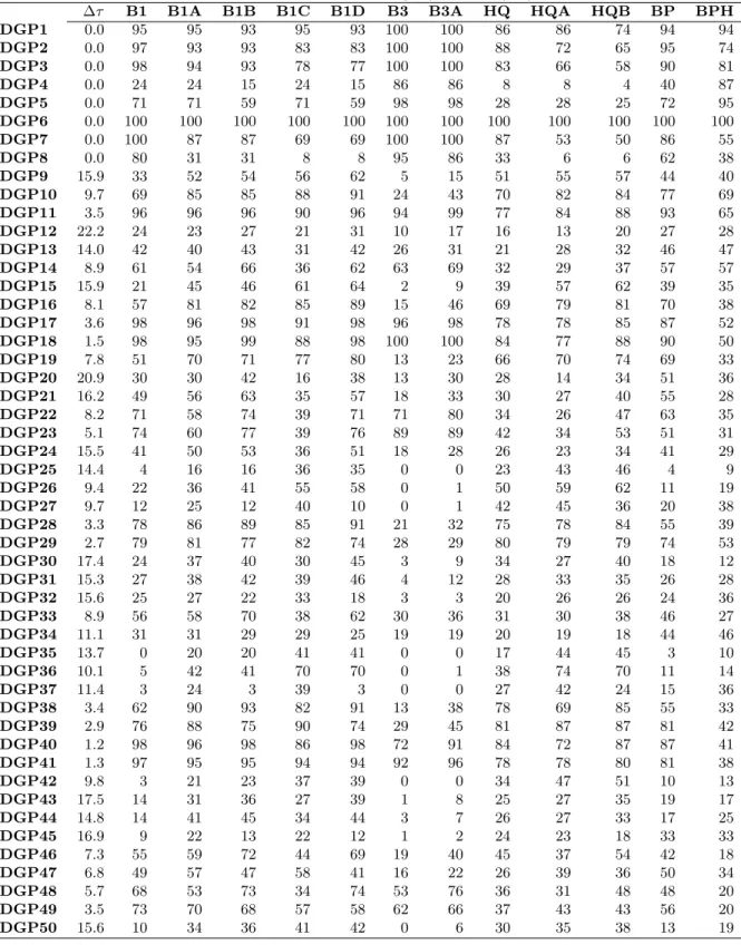
Table 3: Performance of structural break identification approaches: CASE I CASE I:Xt∼N(1,1), et∼N(0,1)
∆τ B1 B1A B1B B1C B1D B3 B3A HQ HQA HQB BP BPH
DGP1 0.0 95 95 93 95 93 100 100 86 86 74 94 94 DGP2 0.0 97 93 93 83 83 100 100 88 72 65 95 74 DGP3 0.0 98 94 93 78 77 100 100 83 66 58 90 81 DGP4 0.0 24 24 15 24 15 86 86 8 8 4 40 87 DGP5 0.0 71 71 59 71 59 98 98 28 28 25 72 95 DGP6 0.0 100 100 100 100 100 100 100 100 100 100 100 100 DGP7 0.0 100 87 87 69 69 100 100 87 53 50 86 55 DGP8 0.0 80 31 31 8 8 95 86 33 6 6 62 38 DGP9 15.9 33 52 54 56 62 5 15 51 55 57 44 40 DGP10 9.7 69 85 85 88 91 24 43 70 82 84 77 69 DGP11 3.5 96 96 96 90 96 94 99 77 84 88 93 65 DGP12 22.2 24 23 27 21 31 10 17 16 13 20 27 28 DGP13 14.0 42 40 43 31 42 26 31 21 28 32 46 47 DGP14 8.9 61 54 66 36 62 63 69 32 29 37 57 57 DGP15 15.9 21 45 46 61 64 2 9 39 57 62 39 35 DGP16 8.1 57 81 82 85 89 15 46 69 79 81 70 38 DGP17 3.6 98 96 98 91 98 96 98 78 78 85 87 52 DGP18 1.5 98 95 99 88 98 100 100 84 77 88 90 50 DGP19 7.8 51 70 71 77 80 13 23 66 70 74 69 33 DGP20 20.9 30 30 42 16 38 13 30 28 14 34 51 36 DGP21 16.2 49 56 63 35 57 18 33 30 27 40 55 28 DGP22 8.2 71 58 74 39 71 71 80 34 26 47 63 35 DGP23 5.1 74 60 77 39 76 89 89 42 34 53 51 31 DGP24 15.5 41 50 53 36 51 18 28 26 23 34 41 29 DGP25 14.4 4 16 16 36 35 0 0 23 43 46 4 9 DGP26 9.4 22 36 41 55 58 0 1 50 59 62 11 19 DGP27 9.7 12 25 12 40 10 0 1 42 45 36 20 38 DGP28 3.3 78 86 89 85 91 21 32 75 78 84 55 39 DGP29 2.7 79 81 77 82 74 28 29 80 79 79 74 53 DGP30 17.4 24 37 40 30 45 3 9 34 27 40 18 12 DGP31 15.3 27 38 42 39 46 4 12 28 33 35 26 28 DGP32 15.6 25 27 22 33 18 3 3 20 26 26 24 36 DGP33 8.9 56 58 70 38 62 30 36 31 30 38 46 27 DGP34 11.1 31 31 29 29 25 19 19 20 19 18 44 46 DGP35 13.7 0 20 20 41 41 0 0 17 44 45 3 10 DGP36 10.1 5 42 41 70 70 0 1 38 74 70 11 14 DGP37 11.4 3 24 3 39 3 0 0 27 42 24 15 36 DGP38 3.4 62 90 93 82 91 13 38 78 69 85 55 33 DGP39 2.9 76 88 75 90 74 29 45 81 87 87 81 42 DGP40 1.2 98 96 98 86 98 72 91 84 72 87 87 41 DGP41 1.3 97 95 95 94 94 92 96 78 78 80 81 38 DGP42 9.8 3 21 23 37 39 0 0 34 47 51 10 13 DGP43 17.5 14 31 36 27 39 1 8 25 27 35 19 17 DGP44 14.8 14 41 45 34 44 3 7 26 27 33 17 25 DGP45 16.9 9 22 13 22 12 1 2 24 23 18 33 33 DGP46 7.3 55 59 72 44 69 19 40 45 37 54 42 18 DGP47 6.8 49 57 47 58 41 16 22 26 39 36 50 34 DGP48 5.7 68 53 73 34 74 53 76 36 31 48 48 20 DGP49 3.5 73 70 68 57 58 62 66 37 43 43 56 20 DGP50 15.6 10 34 36 41 42 0 6 30 35 38 13 19
Note: This table summarizes the performance of the structural break identification approaches for CASE I. The approaches are described at the beginning of Section 4, and the DGPs and the distribution assumption of CASE I are described in Section 4.1. The figures in columns 3 to 9 are the probability of correct detection in percentage. “∆τ” is the average distance between the true break dates and the estimated break dates.
Table 4: Performance of structural break identification approaches: CASE II CASE II: Xt∼N(0,1), et∼N(0,1)
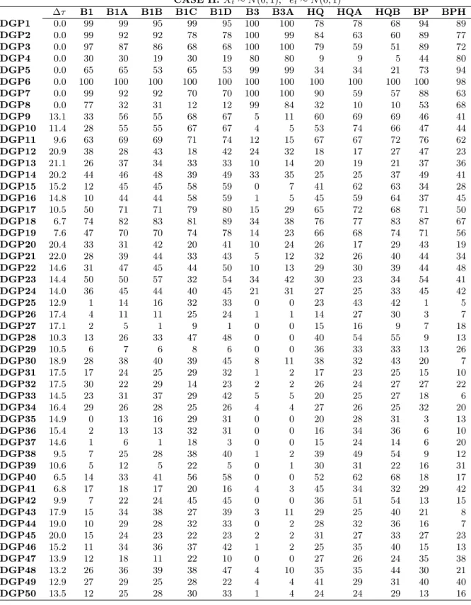
∆τ B1 B1A B1B B1C B1D B3 B3A HQ HQA HQB BP BPH
DGP1 0.0 99 99 95 99 95 100 100 78 78 68 94 89 DGP2 0.0 99 92 92 78 78 100 99 84 63 60 89 77 DGP3 0.0 97 87 86 68 68 100 100 79 59 51 89 72 DGP4 0.0 30 30 19 30 19 80 80 9 9 5 44 80 DGP5 0.0 65 65 53 65 53 99 99 34 34 21 73 94 DGP6 0.0 100 100 100 100 100 100 100 100 100 100 100 98 DGP7 0.0 99 92 92 70 70 100 100 90 59 57 88 63 DGP8 0.0 77 32 31 12 12 99 84 32 10 10 53 68 DGP9 13.1 33 56 55 68 67 5 11 60 69 69 46 41 DGP10 11.4 28 55 55 67 67 4 5 53 74 66 47 44 DGP11 9.6 63 69 69 71 74 12 15 67 67 72 76 62 DGP12 20.9 38 28 43 18 42 24 32 18 17 27 47 23 DGP13 21.1 26 37 34 33 33 10 14 20 19 21 37 36 DGP14 20.2 44 46 48 39 49 33 35 25 25 37 49 41 DGP15 15.2 12 45 45 58 59 0 7 41 62 63 34 28 DGP16 14.8 10 44 44 58 59 1 5 45 59 64 37 45 DGP17 10.5 50 71 71 79 80 15 29 65 72 68 71 50 DGP18 6.7 74 82 83 81 89 34 38 76 77 83 87 67 DGP19 7.6 47 70 70 74 78 14 23 66 68 74 71 56 DGP20 20.4 33 31 42 20 41 10 24 26 17 29 43 19 DGP21 22.0 28 39 44 33 43 5 12 32 26 40 44 34 DGP22 14.6 31 47 45 44 50 10 13 29 30 39 44 48 DGP23 14.4 50 50 57 32 54 34 42 30 23 34 54 41 DGP24 14.0 36 45 44 40 45 21 31 27 25 33 45 42 DGP25 12.9 1 14 16 32 33 0 0 23 43 42 1 5 DGP26 17.4 4 11 11 25 24 1 1 14 27 30 3 7 DGP27 17.1 2 5 1 9 1 0 0 15 16 9 7 18 DGP28 10.3 13 26 33 47 48 0 0 40 54 55 9 13 DGP29 10.5 6 7 6 8 6 0 0 36 33 33 13 26 DGP30 18.9 28 38 40 39 45 8 11 38 32 43 20 7 DGP31 17.5 17 24 25 29 32 1 2 17 23 25 15 10 DGP32 17.5 30 22 29 14 23 2 2 26 24 27 27 22 DGP33 14.5 23 31 37 29 42 5 5 20 25 27 18 6 DGP34 16.4 29 26 28 25 26 4 4 27 26 25 32 20 DGP35 14.9 0 13 16 29 31 0 0 20 28 31 3 13 DGP36 15.4 2 13 13 32 31 0 0 16 34 36 6 10 DGP37 14.6 1 6 1 18 3 0 0 15 24 14 6 20 DGP38 9.5 7 25 28 38 40 1 2 39 49 54 9 12 DGP39 10.6 5 12 5 22 5 0 1 30 31 22 16 31 DGP40 6.5 14 33 41 56 58 0 0 52 62 68 18 17 DGP41 6.8 17 18 17 20 16 4 3 45 34 32 29 42 DGP42 9.9 7 22 24 45 45 0 0 36 51 54 13 15 DGP43 17.9 15 34 38 27 39 3 11 29 25 40 21 8 DGP44 19.0 10 29 28 32 33 0 2 28 32 36 16 7 DGP45 20.0 15 24 23 22 23 2 2 31 27 33 27 23 DGP46 15.2 11 34 36 37 42 1 2 25 35 40 15 13 DGP47 13.9 12 18 11 22 10 0 0 27 26 24 35 38 DGP48 13.2 26 36 39 38 47 4 10 35 35 44 30 21 DGP49 12.9 27 29 25 28 22 4 4 41 29 31 40 40 DGP50 13.5 12 25 28 30 33 1 4 24 24 29 13 16
Note: This table summarizes the performance of the structural break identification approaches for CASE II. The approaches are described at the beginning of Section 4, and the DGPs and the distribution assumption of CASE II are described in Section 4.1. The figures in columns 3 to 9 are the probability of correct detection in percentage. “∆τ” is the average distance between the true break dates and the estimated break dates.
Table 5: Performance of structural break identification approaches: CASE III CASE III: Xt∼N(1,1), et∼N(0,2)
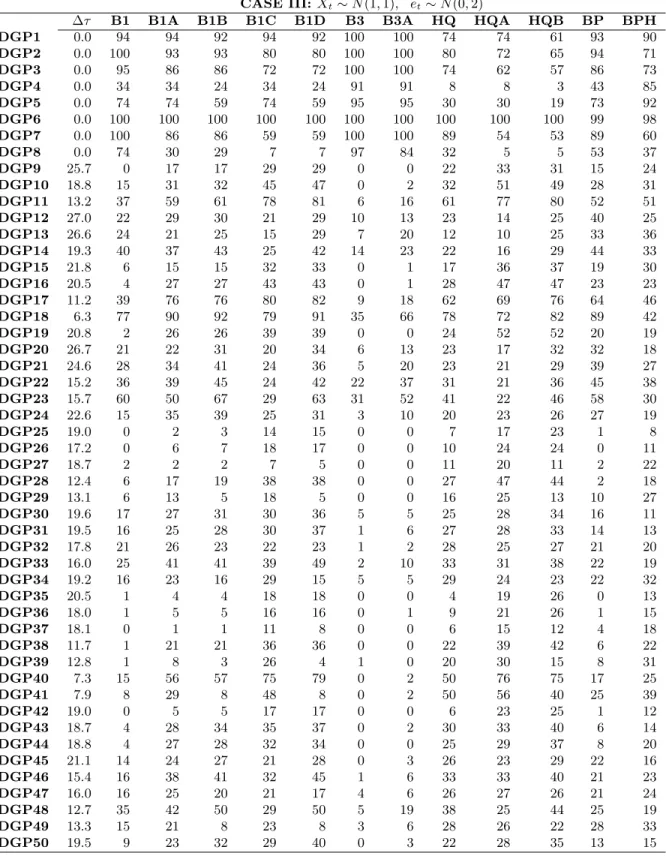
∆τ B1 B1A B1B B1C B1D B3 B3A HQ HQA HQB BP BPH
DGP1 0.0 94 94 92 94 92 100 100 74 74 61 93 90 DGP2 0.0 100 93 93 80 80 100 100 80 72 65 94 71 DGP3 0.0 95 86 86 72 72 100 100 74 62 57 86 73 DGP4 0.0 34 34 24 34 24 91 91 8 8 3 43 85 DGP5 0.0 74 74 59 74 59 95 95 30 30 19 73 92 DGP6 0.0 100 100 100 100 100 100 100 100 100 100 99 98 DGP7 0.0 100 86 86 59 59 100 100 89 54 53 89 60 DGP8 0.0 74 30 29 7 7 97 84 32 5 5 53 37 DGP9 25.7 0 17 17 29 29 0 0 22 33 31 15 24 DGP10 18.8 15 31 32 45 47 0 2 32 51 49 28 31 DGP11 13.2 37 59 61 78 81 6 16 61 77 80 52 51 DGP12 27.0 22 29 30 21 29 10 13 23 14 25 40 25 DGP13 26.6 24 21 25 15 29 7 20 12 10 25 33 36 DGP14 19.3 40 37 43 25 42 14 23 22 16 29 44 33 DGP15 21.8 6 15 15 32 33 0 1 17 36 37 19 30 DGP16 20.5 4 27 27 43 43 0 1 28 47 47 23 23 DGP17 11.2 39 76 76 80 82 9 18 62 69 76 64 46 DGP18 6.3 77 90 92 79 91 35 66 78 72 82 89 42 DGP19 20.8 2 26 26 39 39 0 0 24 52 52 20 19 DGP20 26.7 21 22 31 20 34 6 13 23 17 32 32 18 DGP21 24.6 28 34 41 24 36 5 20 23 21 29 39 27 DGP22 15.2 36 39 45 24 42 22 37 31 21 36 45 38 DGP23 15.7 60 50 67 29 63 31 52 41 22 46 58 30 DGP24 22.6 15 35 39 25 31 3 10 20 23 26 27 19 DGP25 19.0 0 2 3 14 15 0 0 7 17 23 1 8 DGP26 17.2 0 6 7 18 17 0 0 10 24 24 0 11 DGP27 18.7 2 2 2 7 5 0 0 11 20 11 2 22 DGP28 12.4 6 17 19 38 38 0 0 27 47 44 2 18 DGP29 13.1 6 13 5 18 5 0 0 16 25 13 10 27 DGP30 19.6 17 27 31 30 36 5 5 25 28 34 16 11 DGP31 19.5 16 25 28 30 37 1 6 27 28 33 14 13 DGP32 17.8 21 26 23 22 23 1 2 28 25 27 21 20 DGP33 16.0 25 41 41 39 49 2 10 33 31 38 22 19 DGP34 19.2 16 23 16 29 15 5 5 29 24 23 22 32 DGP35 20.5 1 4 4 18 18 0 0 4 19 26 0 13 DGP36 18.0 1 5 5 16 16 0 1 9 21 26 1 15 DGP37 18.1 0 1 1 11 8 0 0 6 15 12 4 18 DGP38 11.7 1 21 21 36 36 0 0 22 39 42 6 22 DGP39 12.8 1 8 3 26 4 1 0 20 30 15 8 31 DGP40 7.3 15 56 57 75 79 0 2 50 76 75 17 25 DGP41 7.9 8 29 8 48 8 0 2 50 56 40 25 39 DGP42 19.0 0 5 5 17 17 0 0 6 23 25 1 12 DGP43 18.7 4 28 34 35 37 0 2 30 33 40 6 14 DGP44 18.8 4 27 28 32 34 0 0 25 29 37 8 20 DGP45 21.1 14 24 27 21 28 0 3 26 23 29 22 16 DGP46 15.4 16 38 41 32 45 1 6 33 33 40 21 23 DGP47 16.0 16 25 20 21 17 4 6 26 27 26 21 24 DGP48 12.7 35 42 50 29 50 5 19 38 25 44 25 19 DGP49 13.3 15 21 8 23 8 3 6 28 26 22 28 33 DGP50 19.5 9 23 32 29 40 0 3 22 28 35 13 15
Note: This table summarizes the performance of the structural break identification approaches for CASE III. The approaches are described at the beginning of Section 4, and the DGPs and the distribution assumption of CASE III are described in Section 4.1. The figures in columns 3 to 9 are the probability of correct detection in percentage. “∆τ” is the average distance between the true break dates and the estimated break dates.
Table 6: Performance of structural break identification approaches: CASE IV CASE IV:Xt∼N(0,1), et∼N(0,2)
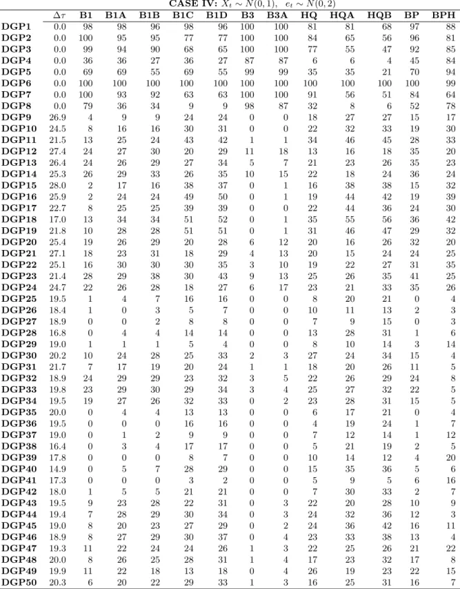
∆τ B1 B1A B1B B1C B1D B3 B3A HQ HQA HQB BP BPH
DGP1 0.0 98 98 96 98 96 100 100 81 81 68 97 88 DGP2 0.0 100 95 95 77 77 100 100 84 65 56 96 81 DGP3 0.0 99 94 90 68 65 100 100 77 55 47 92 85 DGP4 0.0 36 36 27 36 27 87 87 6 6 4 45 84 DGP5 0.0 69 69 55 69 55 99 99 35 35 21 70 94 DGP6 0.0 100 100 100 100 100 100 100 100 100 100 100 99 DGP7 0.0 100 93 92 63 63 100 100 91 56 51 84 64 DGP8 0.0 79 36 34 9 9 98 87 32 8 6 52 78 DGP9 26.9 4 9 9 24 24 0 0 18 27 27 15 17 DGP10 24.5 8 16 16 30 31 0 0 22 32 33 19 30 DGP11 21.5 13 25 24 43 42 1 1 34 46 45 28 33 DGP12 27.4 24 27 30 20 29 11 18 13 16 18 35 20 DGP13 26.4 24 26 29 27 34 5 7 21 23 26 35 23 DGP14 25.3 26 29 33 26 35 10 15 22 18 24 36 24 DGP15 28.0 2 17 16 38 37 0 1 16 38 38 15 32 DGP16 25.9 2 24 24 49 50 0 1 19 44 42 19 39 DGP17 22.7 8 25 25 39 39 0 0 22 44 36 24 30 DGP18 17.0 13 34 34 51 52 0 1 35 55 56 36 42 DGP19 21.8 10 28 28 51 51 0 1 31 46 47 29 32 DGP20 25.4 19 26 29 20 28 6 12 20 16 26 32 20 DGP21 27.1 18 23 31 18 29 4 13 20 15 24 24 25 DGP22 25.1 16 30 30 30 35 3 10 19 22 27 31 35 DGP23 21.4 28 29 38 30 43 9 13 25 26 35 41 25 DGP24 24.7 22 26 28 18 27 6 17 23 21 33 35 26 DGP25 19.5 1 4 7 16 16 0 0 8 20 21 0 4 DGP26 18.4 1 0 3 5 7 0 0 10 11 13 2 3 DGP27 18.9 0 0 2 8 8 0 0 7 9 15 0 3 DGP28 16.8 0 4 4 14 14 0 0 13 28 31 1 6 DGP29 19.0 1 1 1 5 4 0 0 8 10 14 3 14 DGP30 20.2 10 24 28 25 33 2 3 27 24 34 15 4 DGP31 21.7 7 17 19 20 24 1 1 18 20 26 11 5 DGP32 18.9 24 29 29 23 32 3 5 22 26 29 24 8 DGP33 19.8 23 29 30 29 34 3 4 25 27 32 22 5 DGP34 19.5 19 27 26 32 33 0 2 23 28 31 15 5 DGP35 20.0 0 4 4 13 13 0 0 6 17 21 0 4 DGP36 19.5 0 0 0 16 16 0 0 4 19 24 1 7 DGP37 19.0 0 1 2 9 9 0 0 7 12 14 1 12 DGP38 16.4 0 3 4 17 17 0 0 5 21 19 2 5 DGP39 17.8 0 0 0 8 7 0 0 10 14 12 4 20 DGP40 14.9 0 5 7 28 29 0 0 15 35 36 5 6 DGP41 17.3 0 0 0 3 2 0 0 5 9 5 6 16 DGP42 18.0 1 5 5 21 21 0 0 7 30 33 2 7 DGP43 19.5 9 23 28 22 31 0 3 22 20 28 10 9 DGP44 19.4 7 28 29 30 34 0 3 24 32 36 12 3 DGP45 19.0 8 20 23 27 29 0 2 24 36 42 16 11 DGP46 18.9 8 27 29 30 37 0 4 23 33 38 13 4 DGP47 19.3 11 22 24 24 26 1 3 22 25 26 21 22 DGP48 20.0 8 26 25 28 31 1 4 17 23 32 17 8 DGP49 19.9 11 22 18 13 18 0 4 26 19 23 22 15 DGP50 20.3 6 20 22 29 33 1 3 16 25 31 16 7
Note: This table summarizes the performance of the structural break identification approaches for CASE IV. The approaches are described at the beginning of Section 4, and the DGPs and the distribution assumption of CASE IV are described in Section 4.1. The figures in columns 3 to 9 are the probability of correct detection in percentage. “∆τ” is the average distance between the true break dates and the estimated break dates.
Table 7: Mean probability of correct identification of breaks
B1 B1A B1B B1C B1D B3 B3A HQ HQA HQB BP BPH
CASE I:Xt∼N(1,1), et∼N(0,1) K=1, N=1,et∼MA(0) 66 78 78 78 83 41 52 66 74 76 71 58 K=1, N=1,ut∼MA(1) 42 39 45 29 45 33 39 23 23 30 43 44 K=1, N=2,et∼MA(0 65 77 79 80 86 45 55 67 72 78 71 42 K=1, N=2,ut∼MA(1) 53 51 62 33 59 42 52 32 25 42 52 32 K=2, N=1,et∼MA(0) 39 49 47 60 54 10 13 54 61 61 33 32 K=2, N=1,ut∼MA(1) 33 38 41 34 39 12 16 27 27 31 32 30 K=2, N=2,et∼MA(0) 43 60 56 67 64 26 34 55 64 66 43 28 K=2, N=2,ut∼MA(1) 37 46 49 40 47 19 28 31 33 38 35 23 All DGPs except K=0 45 54 56 53 59 27 35 44 47 53 45 33 All DGPs 51 57 58 55 59 38 44 47 48 52 51 40 CASE II: Xt∼N(0,1), et∼N(0,1) K=1, N=1,et∼MA(0) 41 60 60 69 69 7 10 60 70 69 56 49 K=1, N=1,ut∼MA(1) 36 37 42 30 41 22 27 21 20 28 44 33 K=1, N=2,et∼MA(0 39 62 63 70 73 13 20 59 68 70 60 49 K=1, N=2,ut∼MA(1) 36 42 46 34 47 16 24 29 24 35 46 37 K=2, N=1,et∼MA(0) 5 13 13 24 22 0 0 26 35 34 7 14 K=2, N=1,ut∼MA(1) 25 28 32 27 34 4 5 26 26 29 22 13 K=2, N=2,et∼MA(0) 7 18 18 33 29 1 1 32 39 39 13 20 K=2, N=2,ut∼MA(1) 16 29 29 30 31 2 4 30 29 35 25 21 All DGPs except K=0 22 33 34 37 40 7 10 34 38 41 30 27 All DGPs 32 40 40 42 44 21 23 39 40 42 38 36 CASE III:Xt∼N(1,1), et∼N(0,2) K=1, N=1,et∼MA(0) 41 60 60 69 69 7 10 60 70 69 32 35 K=1, N=1,ut∼MA(1) 36 37 42 30 41 22 27 21 20 28 39 31 K=1, N=2,et∼MA(0 39 62 63 70 73 13 20 59 68 70 43 32 K=1, N=2,ut∼MA(1) 36 42 46 34 47 16 24 29 24 35 40 26 K=2, N=1,et∼MA(0) 5 13 13 24 22 0 0 26 35 34 3 17 K=2, N=1,ut∼MA(1) 25 28 32 27 34 4 5 26 26 29 19 19 K=2, N=2,et∼MA(0) 7 18 18 33 29 1 1 32 39 39 8 22 K=2, N=2,ut∼MA(1) 16 29 29 30 31 2 4 30 29 35 18 21 All DGPs except K=0 22 33 34 37 40 7 10 34 38 41 22 24 All DGPs 32 40 40 42 44 21 23 39 40 42 31 32 CASE IV:Xt∼N(0,1), et∼N(0,2) K=1, N=1,et∼MA(0) 8 17 16 32 32 0 0 25 35 35 21 27 K=1, N=1,ut∼MA(1) 25 27 31 24 33 9 13 19 19 23 35 22 K=1, N=2,et∼MA(0 7 26 25 46 46 0 1 25 45 44 25 35 K=1, N=2,ut∼MA(1) 21 27 31 23 32 6 13 21 20 29 33 26 K=2, N=1,et∼MA(0) 1 2 3 10 10 0 0 9 16 19 1 6 K=2, N=1,ut∼MA(1) 17 25 26 26 31 2 3 23 25 30 17 5 K=2, N=2,et∼MA(0) 0 2 3 14 14 0 0 7 20 21 3 10 K=2, N=2,ut∼MA(1) 9 24 25 25 30 0 3 22 27 32 16 10 All DGPs except K=0 9 18 19 24 27 2 4 18 25 29 17 16 All DGPs 21 27 28 31 33 17 18 25 29 31 27 27
Note: This table provides the mean probability of correct identification for the sub-samples defined in the first column. For example, “K=1, N=1,et∼MA(0)” means the DGPs with one break, one covariate, and uncorrelated error terms.
Table 8: Probability of correct identification of partial breaks
BREAKS CASE I CASE IV
C X1 X2 B1A B1C B3A HQA B1A B1C B3A HQA
DGP9 1 0 77 79 87 80 78 75 NA 62 DGP10 0 1 88 88 88 88 81 73 NA 68 DGP11 1 1 81 77 81 79 64 51 00 45 DGP12 1 0 87 81 76 85 89 80 89 75 DGP13 0 1 70 68 77 59 27 30 14 37 DGP14 1 1 67 67 62 76 28 27 27 33 DGP15 1 0 0 73 74 78 50 59 55 100 36 DGP16 0 1 0 89 92 100 93 79 63 100 57 DGP17 0 1 1 77 66 79 82 20 13 NA 20 DGP18 1 1 1 63 63 64 66 18 6 100 18 DGP19 0 1 1 79 68 87 76 36 14 0 18 DGP20 1 0 0 67 63 77 50 62 65 67 45 DGP21 0 1 0 66 80 58 67 22 22 15 33 DGP22 0 1 1 40 23 48 54 10 10 10 14 DGP23 1 1 1 37 38 42 35 14 7 0 22 DGP24 0 1 1 46 42 39 57 8 0 6 17 DGP25 1 0 88 75 NA 67 100 94 NA 65 DGP26 0 1 75 82 100 83 NA 60 NA 63 DGP27 0 1 100 100 100 100 NA 50 NA 43 DGP28 1 1 64 60 84 62 50 36 NA 44 DGP29 1 1 91 84 93 91 00 40 NA 45 DGP30 1 0 97 93 78 96 100 100 100 96 DGP31 0 1 42 51 42 53 18 5 100 23 DGP32 0 1 89 85 67 88 17 13 40 29 DGP33 1 1 48 50 36 53 7 3 0 7 DGP34 1 1 84 76 89 89 37 22 0 21 DGP35 1 0 0 65 71 NA 57 75 69 NA 39 DGP36 0 1 0 74 80 100 77 NA 69 NA 55 DGP37 0 1 0 96 97 NA 93 100 44 NA 33 DGP38 0 1 1 23 11 47 54 33 0 NA 23 DGP39 0 1 1 98 93 96 95 NA 0 NA 40 DGP40 1 1 1 41 28 40 53 0 0 NA 7 DGP41 1 1 1 81 77 81 69 NA 33 NA 33 DGP42 0 1 1 71 49 NA 70 20 5 NA 17 DGP43 1 0 0 97 85 100 79 91 95 100 75 DGP44 0 1 0 39 50 43 48 14 10 0 12 DGP45 0 1 0 73 77 100 87 20 19 0 38 DGP46 0 1 1 20 14 28 32 0 0 0 0 DGP47 0 1 1 82 64 86 79 5 0 0 4 DGP48 1 1 1 25 6 22 26 0 0 0 4 DGP49 1 1 1 81 74 79 77 5 0 0 0 DGP50 0 1 1 15 12 0 22 0 0 0 7
Note: This table provides the probability of correct partial break identification for some selected models and cases. The columns under “BREAKS” indicate the variables subject to breaks (denoted by 1). The figures under a model are the probability that the model correctly identifies the variables subject to breaks when the number of breaks has been correctly identified. Breaks in constant are ignored in determining correct identification: e.g., for DGP11 (where both the constant andX1 are subject to breaks), the case when the constant and X1 are identified to experience breaks and the case when onlyX1 is identified to experience breaks are both considered to be correct identification.