Fiscal consolidation and its cross-country effects

Philippopoulos, A., Varthalitis, P. and Vassilatos, V. (2017) Fiscal consolidation

and its cross-country effects.

Journal of Economic Dynamics and Control

, 83, pp.

55-106. (doi:

10.1016/j.jedc.2017.07.007

)

There may be differences between this version and the published version. You are

advised to consult the publisher’s version if you wish to cite from it.

http://eprints.gla.ac.uk/145276/

Deposited on: 10 Jul 2018

Enlighten – Research publications by members of the University of Glasgow

Accepted Manuscript

Fiscal consolidation and its cross-country effects

Apostolis Philippopoulos, Petros Varthalitis, Vanghelis Vassilatos PII: S0165-1889(17)30157-4

DOI: 10.1016/j.jedc.2017.07.007

Reference: DYNCON 3458

To appear in: Journal of Economic Dynamics & Control

Received date: 8 July 2016 Revised date: 19 July 2017 Accepted date: 20 July 2017

Please cite this article as: Apostolis Philippopoulos, Petros Varthalitis, Vanghelis Vassilatos, Fiscal consolidation and its cross-country effects, Journal of Economic Dynamics & Control (2017), doi:

10.1016/j.jedc.2017.07.007

This is a PDF file of an unedited manuscript that has been accepted for publication. As a service to our customers we are providing this early version of the manuscript. The manuscript will undergo copyediting, typesetting, and review of the resulting proof before it is published in its final form. Please note that during the production process errors may be discovered which could affect the content, and all legal disclaimers that apply to the journal pertain.

ACCEPTED MANUSCRIPT

Fiscal consolidation and its cross-country effects

∗

Apostolis Philippopoulos

†

(Athens University of Economics and Business, and CESifo)

Petros Varthalitis

(Economic and Social Research Institute, and Trinity College Dublin)

Vanghelis Vassilatos

(Athens University of Economics and Business)

July 31, 2017

Abstract

We build a new Keynesian DSGE model consisting of two heterogeneous countries in a monetary union. We study how public debt consolidation in a country with high debt (like Italy) affects welfare in a country with solid public finances (like Germany). Our results show that debt consolidation in the high-debt country benefits the country with solid public finances over all time horizons, while, in Italy, debt consolidation is productive in the medium and long term. All this is with optimized feedback policy rules. On the other hand, fiscal consolidation hurts both countries and all the time, if it is implemented in an ad hoc way, like an increase in taxes. The least distorting fiscal mix from the point of view of both countries is the one which, during the early phase of pain, Italy cuts public consumption spending to address its debt problem and, at the same time, reduces income tax rates, while, once its debt has been reduced in the later phase, it uses the fiscal space to further cut income taxes.

Keywords: Debt consolidation, country spillovers, feedback policy rules, new Keynesian. JEL classification: E6, F3, H6

∗_{We thank the coeditor, James Bullard, and two anonymous referees for many constructive comments.} We thank Konstantinos Angelopoulos, Fabrice Collard, Harris Dellas, George Economides, Saqib Jafarey, Jim Malley, Dimitris Papageorgiou, Evi Pappa, Lefteris Roubanis and Elias Tzavalis for discussions. We thank Johannes Pfeifer for help with Dynare when this paper started. We have benefited from comments by seminar participants at the University of Bern, CESifo in Munich, University of Zurich, City University in London and the Athens University of Economics and Business. Any errors are ours. Petros Varthalitis clarifies that the views expressed here may differ from those of ESRI.

†_{Corresponding author: Apostolis Philippopoulos, Department of Economics, Athens University of} Eco-nomics and Business, Athens 10434, Greece. tel:+30-210-8203357. email: aphil@aueb.gr

ACCEPTED MANUSCRIPT

1

Introduction

Since the global shock of 2008, several eurozone periphery countries have been in a multiple crisis. In view of debt sustainability concerns and loss of confidence, these countries have been forced, among other things, to take restrictive fiscal policy measures which have further dampened demand in the short term. It is thus not surprising that fiscal consolidation has been one of the most debated policy areas over the past years. On the other hand, fiscal policy in eurozone center countries, like Germany, has been neutral. Nevertheless, the debt crisis in the periphery countries has also affected the German economy, which is another reminder of the importance of spillovers in an integrated area like the euro area.1

In this paper, we study how public debt consolidation in a country with high debt and sovereign premia affects welfare in other countries with solid public finances. In particular, we study how public debt consolidation in a country like Italy affects welfare in a country like Germany and how these cross-border effects depend on the fiscal policy mix chosen to bring public debt down.2

The setup is a new Keynesian DSGE model consisting of two heterogeneous countries forming a currency union. An international asset market allows private agents across countries to borrow from, or lend to, each other and the same market allows national governments to sell their bonds to foreign private agents. Regarding macroeconomic policy, being in a monetary union, there is a single monetary policy. On the other hand, the two countries are free to follow independent or national fiscal policies. Following most of the literature on debt consolidation (see below), we follow a rules-based approach to policy. Policy is conducted via ”simple, implementable and optimized” feedback rules (see e.g. Schmitt-Groh´e and Uribe, 2007). This means that the union-wide monetary policy is conducted via a standard Taylor rule for the nominal interest rate, while all the main national fiscal instruments (government consumption spending, government investment spending, transfer payments, and the tax rates on labor income, capital income and consumption) can respond to the gap between public debt and target public debt as shares of output, as well as to the output gap. The values of feedback (monetary and fiscal) policy coefficients are computed optimally, so as to maximize a weighted average of households’ expected discounted lifetime utility in the two countries;

1_{For the debt problem in the euroarea and fiscal policy in various member countries, see e.g. the EEAG}

Report on the European Economy (2012, 2017) by CESifo and EMU-Public Finances (2016) by the European Commission.

2_{Italy’s (public and foreign) debt position, although sizeable in absolute terms, is not one of the worst in}

the euroarea. Greece, Portugal, Spain, Ireland and Cyprus, have been in a worse position; see e.g. the EEAG Report on the European Economy (2012) by CESifo. However, since these countries have received financial aid from the EC-ECB-IMF, we prefer to use Italy as our euro area periphery country.

ACCEPTED MANUSCRIPT

this can be thought of as a cooperative policy at international level. We will experiment with various public debt policy targets depending on whether national policymakers aim just to stabilize the economy around its status quo (defined as the solution consistent with the recent data), or whether they also want to move the economy to a new reformed steady state (defined as a solution with lower public debt than in the recent data). For comparison, we will also study exogenous fiscal consolidation scenarios resembing those recently observed in Italy.

We solve the above model numerically employing commonly used parameter values and fiscal policy data from Germany (called the domestic country) and Italy (called the foreign country). The steady state solution of this model can mimic relatively well the key features of the two countries over the euro years and, more importantly, the current account deficits in Italy financed by current account surpluses in Germany over the period 2001-2011. It is useful to stress that this is achieved simply by allowing for differences in fiscal policy and the degree of patience; the latter means that Italians have been less patient than Germans during the euro period. In turn, we use this solution as a point of departure to study the dynamic evolution of endogenous variables in response to policy reforms, focusing on debt consolidation in the high-debt country, namely, Italy.

Our main results are as follows. First, as perhaps expected, had tax-spending policy in Italy remained unchanged as in the data averages over 2001-2011, the model would be dynamically unstable. In other words, some type of fiscal reaction (spending cuts and/or tax rises) to public debt imbalances was necessary for restoring dynamic stability.

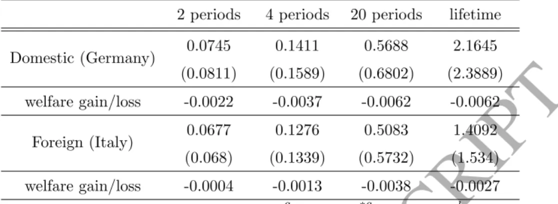
Second, debt consolidation in the high-debt country (Italy) benefits the country with solid public finances (Germany) over all time horizons. By constrast, in Italy, namely the country that takes the consolidation measures, such a policy is productive only in the medium and long term. Thus, in Italy, although the benefits outweigh the costs when the criterion is lifetime utility, debt consolidation comes at a short-term pain relative to non-consolidation. To put it differently, fiscal consolidation in a high debt country is a common interest over longer horizons but, in shorter horizons, there seems to be a conflict of national interests. It is interesting to add that the medium- and long-term benefits from fiscal consolidation become more substantial for both countries when debt reduction is such that sovereign premia are also eliminated in the new reformed steady state; but such elimination requires an equalization of time discount factors, meaning an equal degree of patience, across countries in the new reformed steady state (see section 2.1 for details). All this holds with optimized feedback policy rules.

Third, the least distorting fiscal policy mix from the point of view of both countries is the one where, during the early phase of pain, Italy cuts government consumption spending to

ACCEPTED MANUSCRIPT

address its public debt problem and, at the same time, reduces (labor and capital) income tax rates to mitigate the short-term recessionary effects of these spending cuts, while, once its public debt has been reduced in the later phase, it uses the fiscal space created to further cut capital taxes. In other words, regarding the early phase of pain, Italy’s public debt should be brought down by cuts in government consumption spending only (and not by cuts in govern-ment investgovern-ment and transfer paygovern-ments or by rises in various taxes), while, regarding the later phase of fiscal gain, the anticipation of cuts in capital taxes in the future, once debt consoli-dation has been achieved, plays a key role even in the short term. Use of public consumption spending is also recommended in Germany, where the policy aim is just cyclical stabilization. It is also interesting to report that, to the extent that policy reactions are chosen cooperatively, the higher the say of Germany in policy setting, the stronger the fiscal consolidation in Italy should be during the early period of pain. Again, all this holds with optimized feedback policy rules.

The fourth result is about exogenous data-mimicking policies, so it is a positive result. The implications of such policies are very different from the normative implications listed above. In particular, we experiment with an exogenous scenario of debt consolidation that resembles the policy actually implemented between 2012 and 2015; this means that, in Italy, the tax revenue to GDP ratio rises by around two percentage points, while the spending ratio remains practically unchanged, and, in Germany, fiscal policy is kept neutral. In this case, debt consolidation in Italy is harmful for both countries and across all time horizons, always relative to non-consolidation. Therefore, the way public debt is brought down is important.

Finally, the above results are robust to a number of extensions, namely, the introduction of non-Ricardian households, shocks to starting public debt, changes in the value of the pub-lic debt popub-licy target, or flexible exchange rates. The popub-licy recipes are also robust to the degree of international cooperation in policy decision-making. However, in a non-cooperative (Nash) policy regime, the absence of cooperation leads to a relatively small degree of fiscal consolidation in Italy; the idea is that countries free ride on other countries’ debt stabilization efforts.

The literature closest to our work is the one on debt consolidation in multi-country open economy models and especially in currency union models; see e.g. Coenen et al. (2008), Forni et al. (2010), Clinton et al. (2011), Erceg and Lind´e (2013) and Cogan et al. (2013). These papers have compared different ad hoc fiscal consolidation scenarios in a currency union. Here, by contrast, we compute optimized feedback policy rules for a rich menu of fiscal instruments

ACCEPTED MANUSCRIPT

allowed to be used simultaneously;3 hence, we do not have to make any arbitrary assump-tions about which instrument to use to react to economic condiassump-tions and/or how strong this reaction is (the latter also determines the optimal speed of fiscal consolidation).4 _{We also}

compare optimal to exogenous data-mimicking policy in light of the European debt crisis and thus emphasize the importance of the policy mix adopted. In addition, in what concerns the framework we work within, as far as we know, there have been no previous attempts to search for the best possible use of all main fiscal policy instruments in a new Keynesian DSGE model of a currency union consisting of two heterogeneous countries and, then, study the cross-border implications of fiscal consolidation measures taken by a high-debt country. Country hetero-geneity takes the form of weak public finances and external debt in one country (e.g. Italy) and sound public finances and external assets in the other country (e.g. Germany) and this is reflected in sovereign premia. This type of heterogeneity is at the heart of the current de-bate in Europe and hence allows for a more realistic assessment of alternative consolidation policies. Finally, we also address how the political power of each country affects the chosen consolidation policies in a cooperative international setup, as well as the implications of the lack of such cooperation.5

The rest of the paper is organized as follows. Section 2 presents the model. The status quo solution is in section 3. Section 4 explains our policy experiments. The main results are in sections 5 and 6. Section 7 studies other policy regimes. Section 8 closes the paper. An online appendix provides algebraic details and extra results.

3_{Papers that also compute optimized feedback policy rules in various economic environments include}

Schmitt-Groh´e and Uribe (2005 and 2007), Beetsma and Jensen (2005), Kollmann (2008), Cantore et al. (2017) and Philippopoulos et al. (2015, 2016). Differences from these papers are discussed right below, while alternative approaches to policy decision-making are discussed in the last section (section 8).

4_{As is widely recognized (see e.g. Coenen et al., 2012, and D’ Erasmo et al., 2016), the assumed size of}

feedback policy coefficients is an important factor behind the variation of results across models.

5_{Papers on debt consolidation in closed economy or small open economy models include Bi et al. (2013),}

Corsetti et al. (2013), Almeida et al. (2013), Benigno and Romei (2014), Benigno et al. (2014), Cantore et al. (2017) and Philippopoulos et al. (2015, 2016). Cantore et al. (2017) also study optimized simple rules, as we do here, but this is in a closed economy model, while Philippopoulos et al. (2016) focus on a small open economy. Beetsma and Jensen (2005) and Okano (2014) do compute optimal policies in a currency union but do not study debt consolidation. The literature on debt consolidation has built on the earlier literature on the fiscal-monetary policy interaction; see e.g. Leeper (1991), Schmitt-Groh´e and Uribe (2005 and 2007), Beetsma and Jensen (2005), Kollmann (2008), Leith and Wren-Lewis (2008), Batini et al. (2009), Leeper et al. (2009), Kirsanova et al. (2009), Bi and Kumhof (2011) and Kirsanova and Wren-Lewis (2012).

ACCEPTED MANUSCRIPT

2

A two-country model of a monetary union

This section presents a New Keynesian DSGE model of a currency union consisting of two heterogeneous countries.6

2.1

Informal description of the model

In each country, there are households, firms and a national fiscal authority. In a monetary union, there is a single monetary authority. Households in each country save in the form of physical capital, domestic government bonds and internationally traded assets. The market for internationally traded assets allows private agents across countries to borrow from, or lend to, each other and it also allows national governments to sell their bonds to foreign private agents.7

International borrowing/lending takes place through a financial intermediary or bank and this intermediation requires a transaction cost proportional to the amount of the nation’s debt.8 This cost creates a wedge between the borrowing and the lending interest rate, so that, when they participate in the international asset market, agents (private and public) of the debtor country face a higher interest rate than agents (private and public) of the creditor country.9 To the extent that the bank makes a profit, this profit is rebated lump-sum to households located in the creditor country.

Systematic borrowing and lending cannot occur in an homogeneous world. Some type of heterogeneity is needed. A popular way of producing borrowers and lenders has been to assume that agents differ in their patience to consume; specifically, the discount factor of lenders is higher than that of borrowers or, equivalently, borrowers are more impatient than lenders.10 Such differences in discount factors need to be combined with an imperfection in the capital market in order to get a well-defined solution;11 _{in our model, the capital market imperfection}

is the transaction cost of the loan. Therefore, the international transaction cost ensures, not only stationarity of foreign asset positions as is typically the case in the literature (see e.g.

6_{The model is similar to that in Economides et al (2016). However, here we study optimal debt consolidation}

policies within a currency union, while that paper compared a currency union to other regimes like a fiscal (transfer) union and without optimal policy.

7_{See also Forni et al. (2010), Cogan et al. (2013), Erceg and Lind´e (2013) and many others.}

8_{Thus, as in e.g. C´urdia and Woodford (2010, 2011) and Benigno et al (2014), we use the device of a financial}

intermediary. We could instead assume transaction costs incurred upon borrowers; see e.g. Forni et al. (2010), Cogan et al. (2013), Erceg and Lind´e ( 2013).

9_{That is, here, differences in interest rates across countries are produced by transcation costs incurred by}

the bank. As is known such differences can be produced in various other ways (see subsection 2.5 below).

10_{See also e.g. Benigno et al. (2014). Kiyotaki and Moore (1997) also use a general equilibrium model with}

two types of agents, creditors and borrowers, who discount the future differently. Note that we could further enrich our model so as the discount factors are formed endogenously.

ACCEPTED MANUSCRIPT

Schmitt-Groh´e and Uribe, 2003), but also allows for a well-defined solution with different discount factors across different countries.

The solution of this model will imply that one country (Germany) is a net lender and the other (Italy) is a net borrower in the international asset market and that interest rates are higher in the net debtor country. That is, as said in the Introduction, the relatively impatient Italians finance their current account deficits by borrowing funds from the patient Germans who run current account surpluses. This scenario is also consistent with the literature on the interpretation of current accounts, in the sense that systematic low saving rates and current account deficits are believed to reflect relatively low patience (see e.g. Choi et al., 2008).

On other dimensions, the model is a standard new Keynesian currency union model.12 In particular, each country produces an array of differentiated goods and, in both countries, firms act monopolistically facing Calvo-type nominal fixities. Nominal fixities can give a real role to monetary and exchange rate policy, at least in the transition path. In a monetary union, we assume a single monetary policy but independent national fiscal policies. Policy (both monetary and fiscal) is conducted by optimized state-contingent policy rules.

The rest of this section models the above story. We will present the domestic country. The structure of the foreign country will be analogous except otherwise said. A star will denote the counterpart of a variable in the foreign country.

2.2

Households

This subsection presents the problem of households in the domestic country. There are N identical households indexed byi= 1,2, ..., N. Similarly, in the foreign economy. For simplicity, population in both countries, N andN∗, is constant over time and the two countries are of equal size,N =N∗.

2.2.1 Consumption bundles

The quantity of each varietyh produced at home by domestic firm h and consumed by each domestic household i is denoted as cH_i,t(h). Using a Dixit-Stiglitz aggregator, the composite of domestic goods consumed by each domestic householdi, cH

i,t, consists of h varieties and is

given by:13 cH_i,t = _PN h=1 [cH_i,t(h)]φ−φ1 φ φ−1 (1)

12_{See Okano (2014) for a review of the related literature dating back to Gal´ı and Monacelli (2005, 2008).} 13_{As in e.g. Blanchard and Giavazzi (2003), we work with summations rather than with integrals.}

ACCEPTED MANUSCRIPT

whereφ >0 is the elasticity of substitution across goods produced in the domestic country.

Similarly, the quantity of each imported variety f produced abroad by foreign firmf and consumed by each domestic householdiis denoted ascF

i,t(f). Using a Dixit-Stiglitz aggregator,

the composite of imported goods consumed by each domestic household i, cF_i,t, consists of f varieties and is given by:

cF_i,t = " N P f=1 [cF_i,t(f)]φ−φ1 # φ φ−1 (2)

In turn, having definedcH

i,t andcFi,t, i’s consumption bundle, ci,t, is defined as:

ci,t = cH i,t ν cF i,t 1−ν νν_(1−ν)1−ν (3)

whereν is the degree of preference for domestic goods (ifν >1/2, there is a home bias).

2.2.2 Consumption expenditure, prices and terms of trade

Domestic householdi’s total consumption expenditure is:

Ptci,t=PtHcHi,t+PtFcFi,t (4)

wherePt is the consumer price index (CPI),PtH is the price index of home tradables, andPtF

is the price index of foreign tradables (expressed in domestic currency).

Each domestic household’s total expenditure on home goods and foreign goods are:

P_tHcH_i,t= PN h=1 P_tH(h)cH_i,t(h) (5) P_tFcF_i,t = PN f=1 P_tF(f)cF_i,t(f) (6)

whereP_tH(h) is the price of each varietyh produced at home and P_tF(f) is the price of each varietyf produced abroad, both denominated in domestic currency.

We assume that the law of one price holds meaning that each tradable good sells at the same price at home and abroad. Thus,P_tF(f) =StPtH∗(f), whereSt is the nominal exchange

rate (where an increase in St implies a depreciation) and PtH∗(f) is the price of variety f

produced abroad denominated in foreign currency. Note that the terms of trade are defined as PtF

PH t (=

StPtH∗

PH

t ), while the real exchange rate is defined as

StPt∗

Pt . In a currency union, we set St ≡1 at allt.

ACCEPTED MANUSCRIPT

2.2.3 Household’s optimization problem

Each householdiacts competitively to maximize expected discounted lifetime utility,V0:

V0≡E0 ∞

X

t=0

βtU(ci,t, ni,t, mi,t, gt) (7)

whereci,t isi’s consumption bundle as defined above, ni,t isi’s hours of work,mi,t isi’s real

money holdings, gt is per capita utility-enhancing public goods and services provided by the

government, 0< β <1 is domestic agents’ discount factor, and E0 is a rational expectations

operator.

For our numerical solutions, the period utility function will be (see also e.g. Gal´ı, 2008):

ui,t(ci,t, ni,t, mi,t, gt) =

c1_i,t−σ 1−σ −χn n1+_i,tϕ 1 +ϕ +χm m1_i,t−µ 1−µ +χg g_t1−ζ 1−ζ (8) where χ_n, χ_m, χ_g, σ, ϕ, µ, ζ are standard preference parameters, 1/σ is the elasticity of substitution between consumption at two points in time and 1/ϕis the Frisch labour elasticity. The period budget constraint of each household i in the domestic country written in real terms (i.e. nominal variables are divided by the domestic CPI,Pt) is:

(1 +τc t) h_PH t Pt c H i,t+ PF t Pt c F i,t i +PtH

Pt xi,t+bi,t+mi,t+

StPt∗ Pt f h i,t= = 1−τk_t hr_tkPtH Pt ki,t−1+ωei,t i + (1−τn_t)wtni,t+Rt−1P_Pt−_t1bi,t−1+ +Pt−1 Pt mi,t−1+Qt−1 StPt∗ Pt P∗ t−1 P∗ t f h

i,t−1−τli,t+πi,t

(9)

wherexi,tisi’s investment in domestic physical capital,bi,tis the real value ofi’s end-of-period

domestic government bonds,mi,t isi’s end-of period real domestic money holdings, fi,th is the

real value ofi’s end-of-period internationally traded assets denominated in foreign currency (if fh

i,t <0, it denotes private foreign debt), rkt is the real return to ki,t−1 which is i’s

beginning-of-period domestic physical capital,ω_ei,t denotes i’s real dividends received by domestic firms,

wt is the real wage rate, Rt−1 ≥ 1 denotes the gross nominal return to domestic government

bonds betweent₋1 and t, Qt−1≥1 denotes the gross nominal return to international assets

betweent₋1 andt, τl_i,t is real taxes/transfers (if positive, it denotes lump-sum taxes paid to the government; if negative, it denotes transfers received by the government),πi,t is real profits

distributed in a lump-sum fashion to each domestic household by the financial intermediary and 0 _≤ τc_t, τk_t, τn_t < 1 are tax rates on consumption, capital income and labour income respectively.

ACCEPTED MANUSCRIPT

The law of motion of i’s physical capital is:

ki,t= (1−δ)ki,t−1+xi,t− ξ

2 ki,t ki,t−1 −1 2 ki,t−1 (10)

where 0< δ <1 is a depreciation rate andξ≥0 is a parameter capturing adjustment costs. Details on the household’s problem, its first-order conditions and implications for the price bundles are in Appendix 1.

2.3

Firms

This subsection presents the problem of firms in the domestic economy. There areN domestic firms indexed byh= 1,2, ..., N. Each firmhproduces a differentiated tradable good of variety hunder monopolistic competition and Calvo-type nominal fixities.

2.3.1 Demand for the firm’s product

Demand for each producth, denoted as yH

t (h), is (see Appendix 2 for details):

yH_t (h) = PH t (h) PH t −φ Y_tH (11)

whereY_tH denotes total demand in the domestic country.

2.3.2 Firm’s optimization problem

Real profits of each domestic firmhare defined as:

e ωt(h)≡ P H t (h) Pt y H t (h)− P_tH Pt r k tkt−1(h)−wtnt(h) (12)

wherekt−1(h) and nt(h) denote capital and labor inputs chosen by firmh att.

Maximization is subject to the demand function, (11), and the production function:

y_tH(h) =At[kt−1(h)]α[nt(h)]1−α (13)

whereAt is total factor productivity (TFP), whose motion is defined below, and 0< α <1 is

a technology parameter.

In each period, each firm h faces an exogenous probabilityθ of not being able to reset its price. A firmh, which is able to reset its price at timet, chooses its priceP_t#(h) to maximize the sum of discounted expected nominal profits for the nextkperiods in which it may have to keep its price fixed.

ACCEPTED MANUSCRIPT

Details on the firm’s problem and its first-order conditions are in Appendix 2.

2.4

Government budget constraint

The period budget constraint of the consolidated government sector in the domestic country expressed in real and per capita terms is (see Appendix 3 for details):

bt+StP ∗ t Pt f g t +mt =Rt−1P_Pt−_t1bt−1+Qt−1StP ∗ t Pt P∗ t−1 P∗ t f g t−1+ PPt−t1mt−1+ +PtH Pt gt−τ c t(P H t Pt c H t + P F t Pt c F t )−τkt(rtkP H t Pt kt−1+ωet)−τ n twtnt−τlt (14)

wherebt is the end-of-period domestic real public debt held by domestic households,ftg is the

end-of-period domestic real public debt held by foreign households and expressed in foreign prices,14 andmt is the end-of-period stock of real money balances. Also,gt,cHt ,cFt ,kt−1,ωet,nt

are respectively government purchases of goods and services, households’ consumption of the domestic good, households’ consumption of the imported good, households’ physical capital holdings, households’ dividends and household’s work hours. Finally, τc_t, τk_t, τn_t and τl_t have been defined above.

Equivalently, if we define total nominal public debt in the domestic country as Dt ≡

Bt +StFtg, so that in real and per capita terms dt ≡ bt + StP

∗ t Pt f g t, we have bt ≡ λtdt and StPt∗ Pt f g

t ≡ (1−λt)dt, where 0 ≤ λt ≤ 1 denotes the fraction of domestic public debt held by

domestic private agents and 0 _≤ 1₋λt ≤ 1 is the fraction of domestic public debt held by

foreign private agents.

In each period, one of the fiscal instruments (τc_t,τk_t,τn_t, gt, τlt, λt, dt) follows residually to

satisfy the government budget constraint. We assume, except otherwise said, that this role is played by the end-of-period total public debt,dt.15

14_{Since the returns to bonds held by domestic agents and the same bonds held by foreign agents can differ,}

our modelling assumes implicitly that the bond market can be segmented.

15_{We treat the share of public debt held by foreign private agents, (1−λ}

t), as an exogenous variable. In our model, there is a single international asset subject to a single transaction cost. Thus, since we do not allow for separate international asset markets (one for private and one for public), we need an extra assumption to get a solution and this is provided by treatingλt as an exogenous variable in each country (it will be set as in the data average). Alternatively, we could assume that private agents in each country can separately invest in foreign private assets and foreign government bonds (rather than in a single international asset). But, as is known, this modelling would lead to a non-well specified system (a kind of portfolio indeterminacy), except if one is willing to assume different transaction costs in different asset markets. In the latter case, portfolio shares could be determined but their solution would depend on the parameterization of the associated transaction cost function. This would not be different from treatingλt exogenously in the first place.

ACCEPTED MANUSCRIPT

2.5

World financial intermediary

We use a simple and popular model of financial frictions (see e.g. Uribe and Yue, 2006, C´urdia and Woodford, 2010 and 2011, and Benigno et al., 2014). International borrowing, or lending, takes place through a financial intermediary or bank. This intermediary is located in the home country. It plays a traditional role only, collecting deposits from lenders and lending the funds to borrowers.

In particular, the bank raises funds from domestic private agents, fh t −ftg

, at the rate Qt and lends to foreign agents, (ft∗g−ft∗h), at the rate Q∗t.16 In addition, the bank faces

operational costs, which are increasing and convex in the volume of the loan, (f_t∗g−f_t∗h). The profit of the bank is revenue minus cost where revenue is net of transaction costs. Thus, the profit written in real and per capita terms in the domestic country is given by (details are in Appendix 4): πt =Q∗t−1 " Pt−1 Pt (f ∗g t−1−ft∗−h1)− PH t Pt PH t−1 P_tH ψ 2(f ∗g t−1−ft∗−h1)2 # −Qt−1 StPt∗ Pt P_t∗₋₁ P_t∗ f_th₋₁₋f_tg₋₁ (15) where ψ₂(f_t∗₋g₁₋f_t∗₋h₁)2 is a real and per capita cost function and ψ _≥ 0 is a parameter (see subsection 3.1 below for its value). The first term in the brackets on the RHS is the bank’s return on the loan net of transaction costs, while the last term is payments to the savers.

At eacht, the bank chooses the volume of its loan takingQtandQ∗t as given. The optimality

condition is (details are in Appendix 4):

Q∗_t−1= Qt−1 St St−1 1− Pt−H1 Pt−1ψ(f ∗g t−1−ft∗−h1) (16)

where, in a currency union,St≡1; thus,Q∗t > Qt which means that borrowers pay a sovereign

premium.

It needs to be said that the implied property in equation (16) - namely, that the interest rate, at which the country borrows from the rest of the world, is increasing in the nation’s total foreign debt - is supported by a number of empirical studies (see e.g. EMU-Public Finances,

16_Herefh t ≡ PN i=1fi,th N , wheref h i,t≡ Fi,th

Pt∗ is each householdi’s foreign assets denominated in foreign currency,

andftg≡ Ftg

P∗

tN is real and per capita public foreign debt (i.e. public debt held by foreign agents) in the domestic

country; similarly in the foreign country. Then, if it so happens that fh t −ftg

is positive, it denotes net foreign assets in the home country and if it so happens that (ft∗g−ft∗h) is positive, it denotes net foreign liabilities in the foreign country. In equilibrium, (ft∗g−ft∗h) +StP

∗ t

Pt (f

g

ACCEPTED MANUSCRIPT

2012, by the European Commission). It should also be said that a similar type of endogeneity of the country premium can be produced by several other models, including models of default risk.17

2.6

Monetary and fiscal policy

We now specify monetary and fiscal policy rules.

2.6.1 Single monetary policy rule in a monetary union

If we had flexible exchange rates, the exchange rate would be an endogenous variable and the two countries’ nominal interest rates, Rt and R∗t, could be free to be set independently by

the national monetary authorities, say, to follow national Taylor-type rules (see section 7 for flexible exchange rates). Here, by contrast, to mimic the eurozone regime, we assume that only one of the nominal interest rates, say Rt, can follow a Taylor-type rule, while R∗t is an

endogenous variable replacing the exchange rate which becomes an exogenous policy variable (this modelling, where the union’s central bank uses one of national governments’ interest rates as its policy instrument, is similar to that in e.g. Gal´ı and Monacelli, 2008, and Benigno and Benigno, 2008).18

In particular, we assume a single monetary feedback policy rule of the form:

log Rt R = φ_π ηlog Πt Π + (1−η) log Π∗_t Π∗ + +φ_y ηlog yH t yH + (1₋η) log y∗H t y∗H (17)

where φ_{π ≥} 0 and φ_{y ≥} 0 are respectively feedback monetary policy coefficients on price inflation and the output gap, 0≤η ≤1 is the political weight given to the domestic country relative to the foreign country (see subsection 3.1 below for the value of this parameter) and variables without time subscripts denote policy targets (in the case of monetary policy, the policy targets are simply the steady state values of the corresponding variables).

17_{Default risk reflects the fear of de jure, or outright, repudiation of debt obligations, but also the fear of de}

facto default via inflation or new wealth taxes with retroactive effect (see Alesina et al., 1992, for an early study and D’ Erasmo et al., 2016, for a recent study). As Corsetti et al. (2013) point out, there are two modelling approaches to sovereign default. The first approach models it as a strategic choice of the government (see e.g. Eaton and Gersovitz, 1981, Arellano, 2008, D’ Erasmo et al., 2016, and many others). The second approach assumes that default occurs when debt exceeds an endogenous fiscal limit (see e.g. Bi, 2012, and many others). In our paper, we abstract from issues related to default.

18_{For various ways of modelling monetary policy in a monetary union, see e.g. Dellas and Tavlas (2005) and}

ACCEPTED MANUSCRIPT

2.6.2 National fiscal policy rules

Countries can follow independent fiscal policies. As in the case of monetary policy above, we focus on simple feedback rules meaning that national fiscal authorities react to a small number of easily observable macroeconomic indicators. In particular, in each country, we allow all the main spending-tax policy instruments, namely, the ratio of real government spending on goods and services to real GDP, defined as sg_t, the ratio of real government transfers to real GDP, denoted assl

t, and the tax rates on consumption, capital income and labor income, τct,τkt and

τn_t, to react to the public debt-to-GDP ratio as deviation from a target value, as well as to the output gap, according to simple linear rules:19

sg_t −sg=−γg_l (lt−1−l)−γgy ytH−yH (18) sl_t−sl=γl_l(lt−1−l) +γly yHt −yH (19) τc_{t −}τc=γc_l(lt−1−l) +γcy yHt −yH (20) τk_t −τk =γk_l (lt−1−l) +γky ytH−yH (21) τn_{t −}τn =γn_l (lt−1−l) +γny yHt −yH (22)

where lt−1 is the beginning-of-period government liabilities as share of GDP (defined right

below),γq_l andγqy≥0, for q≡(g, l, c, k, n), are respectively feedback fiscal policy coefficients

on public liabilities and the output gap, and variables without time subscripts denote policy targets (see subsection 4.1 below for definition of fiscal policy targets). It should be recalled that a negative value of sl_t denotes transfers, so a positive γl_l means that transfers fall when public liabilities rise above their target.

From the government budget constraint, public liabilities at the end of period texpressed in real and per capita terms are (see Appendix 3 for details):

19_{For similar rules, see e.g Schmitt-Groh´e and Uribe (2007) and Cantore et al. (2017). See also EMU-Public}

Finances (2011) by the European Commission and D’ Erasmo et al. (2016) for fiscal reaction functions used in practice and their role in public debt sustainability.

ACCEPTED MANUSCRIPT

lt ≡ Rtλtdt+QtS_St+1_t (1−λt)dt PH t Pt y H t (23)

Fiscal policy in the foreign country is modelled similarly.

2.7

Exogenous variables and shocks

We now specify the rest of the exogenous variables, At, A∗t, λt, λ∗t and SSt+1t . Starting with

TFP in the two countries,At andA∗t, we assume stochastic AR(1) processes of the form:

log (At) = (1−ρa) log (A) +ρalog (At−1) +εαt (24)

log (A∗_t) = (1−ρ∗a) log (A∗) +ρ∗alog A∗_t−1+ε∗_tα (25) where 0 < ρa, ρ∗a < 1 are persistence parameters, variables without time subscript denote

steady state values andεa_t ∼N 0, σ2_a, ε_t∗a∼N 0, σ∗_a2.

The fiscal policy variables,_{λt, λ∗t}∞t=0, are assumed to be constant and equal to their data

average values in allt. Finally, as said, in a regime of a currency union, we setSt≡1 in all t.

In other words, we assume that stochasticity comes from shocks to TFP only (we report however that our main results do not depend on this).

2.8

Equilibrium system in the status quo economy

We now combine the above to get the equilibrium system for any feasible policy. This is defined to be a sequence of allocations, prices and policies such that: (i) households maximize utility; (ii) a fraction (1−θ) of firms maximize profits by choosing an identical price P_t#, while a fractionθ just set prices at their previous period level; (iii) the international bank maximizes its profit (iv) all constraints, including the government budget constraint and the balance of payments, are satisfied; (v) all markets clear, including the international asset market; (vi) policy instruments are set by feedback rules.

This equilibrium system is presented in detail in Appendix 5. It consists of 61 equations in 61 variables,{Vt, yHt ,ct, cHt , cFt , nt, xt, kt, fth,mt, T Tt,Πt,ΠHt ,Θt, ∆t, wt, mct,ωet, rkt, dt,Π∗t,

z1

t, zt2, πt, qt, Qt, lt, Vt∗, yt∗H, c∗t, cHt ∗, cFt∗, n∗t, xt∗, k∗t, fth∗, m∗t,ΠHt ∗, Θ∗t, ∆∗t, wt∗, mc∗t, ωe∗,

r∗_tk, d∗_t, z1_t∗, z2_t∗, Q_t∗, l_t∗, Rt, stg, slt,τct, τkt, τnt, R∗t , sgt∗, slt∗, τct∗, τkt∗, τnt∗}∞t=0. This is for given

ACCEPTED MANUSCRIPT

feedback policy coefficients as defined in subsection 2.6 (these values will be chosen optimally) and initial conditions for the state variables.

2.9

Plan of the rest of the paper

Our main goal in this paper is to evaluate the implications of various hypothetical and actual debt consolidation policies. We will therefore work as follows. First, using commonly employed parameter values and fiscal data from Germany and Italy, we will numerically solve the above model. This is in the next section (section 3). In turn, to the extent that the steady state solution of this model is empirically relevant (meaning that it can mimic the data averages over the euro area period of study), we will use this solution - defined as the status quo - as a point of departure in order to evaluate the implications of various debt consolidation policies. A description of policy experiments and a discussion of the solution methodology are in section 4, while numerical solutions are in sections 5, 6 and 7.

3

Data, parameteres and solution of the status quo model

This section solves numerically the above model by using annual data from Germany and Italy over the period 2001-2011. We start in 2001 because this year marked the introduction of the euro and we stop at 2011 because the year 2012 marked the beginning of fiscal consolidation efforts in Italy (see e.g. EMU-Public Finances, 2015, by the European Commission).

3.1

Parameter values and fiscal policy variables

The baseline parameter values and the data averages of fiscal policy variables, used in the numerical solution of the above model, are listed in Tables 1a and 1b respectively. The time unit is meant to be a year. The two countries can differ only in their discount factors (seeβ andβ∗ in Table 1a) and fiscal policy variables (see the fiscal policy instruments in Table 1b). In all other respects, the two countries are assumed to be symmetric. Interestingly, as said above, these two differences will prove to be enough to give a steady state solution close to the data averages during 2001-2011.

Regarding parameter values, the model’s key parameters are the discount factors in the two countries,β andβ∗, and the cost coefficient driving the wedge between the borrowing and the lending interest rate,ψ. The values of these parameters are calibrated to match the real interest rates and the net foreign asset position of the two countries in the time period under consideration. In particular, the values ofβandβ∗follow from the Euler equations in the two

ACCEPTED MANUSCRIPT

countries which, at the steady state, are reduced to:

βQ/Π = 1 (26)

β∗Q∗/Π∗ = 1 (27)

whereQ/Π andQ∗/Π∗ are gross real interest rates in the two countries (see Appendix 5 for detailed definitions of all variables). Since Q/Π < Q∗/Π∗ in the data over the period under consideration, it follows β = 0.9833 > β∗ = 0.9780. That is, the Germans are more patient than the Italians.

In turn, the optimality condition of the bank, (16), written at the steady state, is:

Q∗= Q

1− PPHψ(f∗g−f∗h)

(28)

from which the value of the parameterψ is calibrated.

All other parameter values, as listed in Table 1a, are the same across countries and are set at values commonly used in related studies. We start by setting the value of the political weight, η, at the ”neutral” value of 0.5 (a sensitivity analysis regarding this parameter is in section 6 below). We report that our main results are robust to changes in these values (see section 6 below for further details). Thus, although our numerical simulations below are not meant to provide a rigorous quantitative study, they illustrate the qualitative dynamic features of the model in a realistic way.

ACCEPTED MANUSCRIPT

Table 1a: Baseline parameter values

Parameter Home Foreign Description

a, a∗ _{0.3 0.3 share of physical capital in production}

ν, ν∗ 0.5 0.5 home goods bias in consumption

µ, µ∗ 3.42 3.42 money demand elasticity in utility

δ, δ∗ 0.1 0.1 capital depreciation rate

φ, φ∗ 6 6 price elasticity of demand

ϕ, ϕ∗ 1 1 inverse of Frisch labour elasticity

σ, σ∗ 1 1 inverse of elasticity of substitution in consumption

θ, θ∗ 0.2 0.2 price rigidity parameter

χ_m, χ∗

m 0.001 0.001 preference parameter related to money balances

χ_n, χ∗_n 5 5 preference parameter related to work effort

χ_g, χ∗_g 0.1 0.1 preference parameter related to public spending

ξ, ξ∗ 0.01 0.01 adjustment cost parameter of physical capital

ζ, ζ∗ 1 1 public spending elasticity in utility

η 0.5 0.5 political weight in union-wide policies

β, β∗ 0.9833 0.9780 time discount factor

ψ 0.072 - cost parameter in international borrowing

σα, σα∗ 0.01 0.01 standard deviation of TFP ρα, ρα∗ 0.92 0.92 persistence of TFP

Regarding fiscal policy variables in the two countries as defined in subsection 2.6.2 above, the steady state government spending-to-GDP ratios and tax rates are set to their average values in the data in Germany and Italy over 2001-2011 (see Table 1b). In particular, as a measure of sg _{and s}∗g_{, which serve as arguments in households’ utility function and hence}

are typically thought of as public consumption, we use data on total government spending on goods and services,20 _{while, we use data on transfer payments as a measure ofs}l_ands∗l_{, which}

enter households’ budget constraints. As tax rates, τc_{, τ}∗c_{, τ}k_{, τ}∗k_{, τ}n _{and τ}∗n_{, we use the}

associated effective tax rates (or what Eurostat calls implicit tax rates).

20_{We could use data on government consumption spending only to measures}g _{and s}∗g_{; this is not important} to our results. In subsection 6.4 below, we will augment the model by giving different roles to government consumption and government investment spending.

ACCEPTED MANUSCRIPT

Table 1b: Fiscal policy variables (2001-2011 data averages)

Variable Home Foreign Description

τc_{, τ}∗c _{0.1934 0.1756 consumption tax rate}

τk, τ∗k 0.2041 0.3118 capital income tax rate

τn, τ∗n 0.3833 0.421 labour income tax rate

sg_{, s}∗g _{0.2131 0.2423 government purchases of goods/services as share of GDP}

sl_{, s}∗l _{-0.2039 -0.2163 government transfers payments as share of GDP}

λ, λ∗ 0.52 0.61 share of public debt held by domestic agents Note: The data source is Eurostat.

3.2

Steady state solution in the status quo model

The equilibrium system was defined in subsection 2.8 and the associated steady state follows simply if we assume that variables do not change over time (details are at the end of Appendix 5). Table 2 presents the steady state solution when parameters and policy instruments are set at the values in Tables 1a-b. It is worth pointing out that, since policy instruments react to deviations of macroeconomic indicators from their steady state values, feedback policy coefficients do not play any role in steady state solutions. In this steady state solution, the residually determined public financing variable is public debt in both countries. Table 2 also presents some key ratios in the German and Italian data and, as can be seen, the respective ratios implied by the steady state solution are close to their values in the data. In particular, the solution can mimic rather well the data averages of public debt-to-GDP ratios and foreign debt-to-GDP ratios in the two countries over 2001-2011.

This steady state solution will serve as a point of departure. That is, in what follows, we will depart from this solution to study the implications of various policy experiments. We report (and this is confirmed below) that an exogenous reduction in public debt stimulates output and improves welfare in both countries; this can provide a first justification for our fiscal consolidation experiments.

ACCEPTED MANUSCRIPT

Table 2: Status quo steady state solution

Variables Description Home Data Foreign Data

u, u∗ _{utility 0.0376 - 0.0315}

-yH, yH∗ output 0.3912 - 0.3543

-c, c∗ consumption 0.2314 - 0.2278

-n, n∗ hours worked 0.3116 - 0.3063

-k, k∗ capital 0.6655 - 0.4976

-w, w∗ real wage rate 0.6976 - 0.7085

-rk, rk∗ real return to capital 0.1470 - 0.1780

-Q∗₋Q interest rate premium - - 0.0055 0.0055

c yH_{T T}1−ν, c ∗ yH∗_{T T}ν∗−1 t consumption as share of GDP 0.5633 - 0.6752 -k yH, k ∗ yH∗ capital as share of GDP 1.7009 - 1.4045 -d T Tν−1_yH, d ∗ T T1−ν∗_y∗H

total public debt as share of GDP 0.6907 0.6861 1.0871 1.08 _(1−λ)d T T ν−1−T Tν ∗ t fh yH , (1−λ∗)d∗ T T1−ν−ν∗−f ∗h T Tν ty∗H

total foreign debt as share of GDP*

-0.2109 -0.2501 0.2114 0.2109 Notes: Parameters and policy variables as in Tables 1a-b.

3.3

Transition dynamics and determinacy

It is well recognized that the interaction between fiscal and monetary policy, and, in particular, the magnitude of the associated feedback policy coefficients in the policy rules, are crucial to determinacy (see e.g. Leith and Wren-Lewis, 2008). This is also the case in our paper. In particular, when we assume that fiscal policy instruments remain constant at their data average values in Table 1b without any reaction to public debt and there is no interest rate policy reaction to inflation, the model, when approximated around the status quo steady state solution, exhibits dynamic instability meaning that there is no convergence to the steady state solution reported above. In other words, policy can guarantee a unique transition path, only when at least one fiscal policy instrument in each country (sg_t, sl_t, τc_t, τk_t, τn_t andsg_t∗,s_tl∗, τc_t∗, τk_t∗, τn_t∗) reacts to public liabilities. The magnitude of these reactions lies within a range of critical minimum and maximum non-zero values. These critical values differ across different fiscal policy instruments. And all this holds when monetary policy satisfies the so-called Taylor principle, meaning that the single nominal interest rate reacts aggressively to inflation. This will also be confirmed by the results for optimized policy rules below. By contrast, fiscal and

ACCEPTED MANUSCRIPT

monetary policy reaction to the output gap has not been found to be crucial for determinacy. Further details regarding ranges of feedback policy coefficients guaranteeing local determinacy are available upon request. In sum, determinacy requires stabilizing fiscal reaction to inherited public debt and monetary reaction to inflation; this holds in all cases studied below.

4

Description of policy experiments and solution strategy

This section defines our policy experiments and explains the solution strategy. Numerical results will then be presented in sections 5, 6 and 7. In our main thought experiment, we will depart from the status quo steady state solution (in other words, the initial values of the predetermined variables will be those found by the steady state solution in Table 2) and compute the equilibrium transition path as we travel towards a new reformed steady state (the key policy reforms are defined in subsection 4.1). Additional policy scenarios, used mainly for comparison, are defined in subsection 4.2. The values of feedback coefficients of monetary and fiscal policy instruments used in the transition from the status quo steady state to a new steady state will be chosen optimally (this is explained in subsection 4.3). Transition dynamics will be driven by extrinsic TFP shocks in both countries and by policy reforms in the high-debt country, except otherwise said.21

4.1

National fiscal policies and reforms in the main policy experiment

In our main thought experiment, motivated by the facts discussed in the opening paragraph of the Introduction, we focus on two different types of fiscal action, one for each country.

4.1.1 Fiscal policy scenario in the domestic country with solid public finances

The domestic country (defined to be Germany) is assumed to follow a neutral fiscal policy. In other words, we assume that the domestic country does not take any active fiscal consolidation measures but it just stabilizes the public debt-to-GDP ratio at its average level, where the latter, namely the public debt target in the country’s feedback policy rules, is defined to be the steady state value of the public debt-to-GDP ratio as determined residually by the within-period government budget constraint. That is, in this country, we depart from, and end up at, the same tax-spending position, which is as in the average data in Germany (however, as explained below, the new steady state solution will differ from the status quo solution because

21_{We have also experimented with asymmetric shocks (for instance, shocks in one country only), or no shocks}

at all, and the main results do not change. Thus, our main results will be driven by policy (debt consolidation) reforms in the high-debt country.

ACCEPTED MANUSCRIPT

of fiscal consolidation in the foreign country). This is usually called ”debt accommodation” in the related literature (see Wren-Lewis, 2010).

Specifically, fiscal policy in the domestic country is defined as follows: (a) All exogenously set tax-spending national policy instruments remain at the same value (data average value) in both the status quo steady state and the new steady state. (b) Along the transition to the new steady state, all tax-spending national policy instruments are allowed to react to deviations from policy targets in a optimized way (see subsection 4.3 below), where the policy targets are the endogenously determined new steady state values. (c) All the time, namely, both during the transition and in the steady state, the public debt serves as the residually determined public financing instrument closing the within-period government budget constraint.

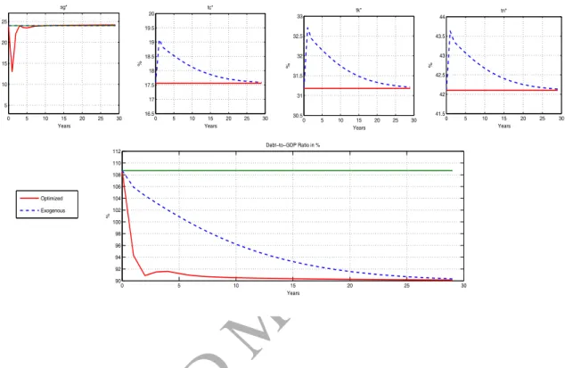
To understand this scenario, imagine that the economy is hit by a temporary adverse shock to TFP as modelled in equations (24)-(25). This, as the impulse response functions can show, leads at impact to a contraction in output and a rise in the public debt-to-output ratio. Then, the policy questions are which tax-spending policy instrument to use over time, and how strong the reaction of those policy instruments to deviations from targets should be, in order to minimize cyclical volatility.

4.1.2 Fiscal policy scenario in the foreign country with weak public finances

The role of fiscal policy in the foreign country (defined to be Italy) is twofold: to stabilize the economy against the same shocks as above and, at the same time, to improve resource allocation by bringing down its public debt-to-GDP ratio over time. This is typically called ”debt consolidation” in the related literature (see Wren-Lewis, 2010).

Specifically, in our main thought experiment, fiscal policy in the foreign country (i.e. Italy) is defined as follows: (a) In the new reformed steady state, the country’s output share of public debt is exogenously set at the target value of 90% (recall that it was around 110% of GDP in the status quo steady state solution in subsection 3.2).22 _{Actually, we will study two subcases}

here: one in which sovereign premia may remain in this reformed steady state, as determined endogenously by equation (28), similarly to the status quo model; and one in which, not only public debt is reduced to 90%, but also sovereign premia are eliminated in the new reformed steady state, meaning that now we also impose Q = Q∗ in equation (28). Obviously, the second case, the one without premia, is more ambitious. Modelling details are provided in

22_{We choose the target value of 90% simply because this is consistent with evidence provided by e.g. Reinhart}

and Rogoff (2010) and Checherita-Westphal and Rother (2012) that, in most advanced economies, the adverse effects of public debt arise when it is around 90-100% of GDP. We report that our main results are not sensitive to this value. For instance, we have experimented with a debt target value of 70% or 60% and the results are qualitatively the same.

ACCEPTED MANUSCRIPT

the next subsection right below. (b) In this new reformed steady state, since the country’s public debt has been reduced and thus fiscal space has been created relative to the status quo, fiscal spending can be increased and/or tax rates can be cut, depending on which fiscal policy instrument is assumed to follow residually to close the government budget constraint. This is known as the long-term fiscal gain from debt consolidation. Here, we will report results only for the case in which the fiscal space created by debt reduction is used to reduce the capital tax rate;23this has been found to be the most efficient way of making use of the fiscal space created and is consistent with the Chamley-Judd well known normative result that the limiting capital tax rate should be zero. To put it differently, our solutions confirm, as in most of the literature, that the impact of debt consolidation depends on expectations about how the fiscal space will be used in the future and it is expectations of a cut in the capital tax rate that appear to have a long-lasting beneficial effect on investment and output. (c) Along the transition to the new reformed steady state, the national tax-spending policy instruments are allowed to react to deviations from policy targets in a optimized way (see subsection 4.3 below). Given that the new debt policy target is set at a value lower than in the status quo (i.e. we depart from 110% but the policy target in Italy’s feedback fiscal policy rules is 90%), this requires lower public spending, and/or higher tax rates, during the early phase of the transition period. This is known as the short-term fiscal pain of debt consolidation.24

4.1.3 Equilibrium system in the reformed economy: modelling issues

The equilibrium system and modelling details are in Appendix 6. As explained in that Appendix, the case in which premia are allowed in the new steady state is similar to the status quo regime in terms of modelling except that in the reformed economy the debt policy target is 90%. On the other hand, the case in which we also set Q= Q∗ in the new steady state is more demanding. In particular, elimination of premia, or equivalently equalization of interest rates, Q = Q∗, means that the international capital market becomes perfect so that agents can borrow and lend at the same interest rate internationally. For this to happen,

23_{Results with other instruments are available upon request.}

24_{It is well recognized that debt consolidation implies a tradeoff between short-term pain and medium-term}

gain; see e.g. Coenen et al. (2008) and Clinton et al. (2011). During the early phase of the transition, debt consolidation comes at the cost of higher taxes and/or lower public spending. In the medium- and long-run, a reduction in the debt burden allows, other things equal, a cut in tax rates, and/or a rise in public spending. Thus, one has to value the early costs of stabilization vis-a-vis the medium- and long-term benefits from the fiscal space created. It is also recognized that the implications of fiscal reforms, like debt consolidation, depend heavily on the public financing policy instrument used, namely, which policy instrument adjusts endogenously to accommodate the exogenous changes in fiscal policy; see e.g. Leeper et al. (2009). In the case of debt consolidation, such implications are expected to depend both on which policy instrument bears the cost of adjustment in the early period of adjustment and on which policy instrument is expected to reap the benefit, once consolidation has been achieved.

ACCEPTED MANUSCRIPT

however, and as discussed in subsection 2.1 above, the discount factors need also to be equalized across countries. Namely, without financial frictions, the agents should become equally patient eventually. Thus,β∗ needs to become equal toβ at the new steady state (although this is not required along the transition). To model this, in a relatively neutral way, we assume that the discount factor in Italy,β∗, follows over time the AR(1) process:

β∗_t =ρβ∗β∗_t−1+1₋ρβ∗β (29) where the initial value is the value used in the status quo solution (see Table 1a) while the value in the new reformed steady state is set as in Germany (see Table 1a again).25 _{It is important to}

stress that, in case premia are eliminated in the new steady state so thatβ∗=β, we will choose the autoregressive parameter, ρβ∗, optimally, alongside all other feedback policy parameters, so as not to force results in one direction or another. In general, ρβ∗ can be thought of as capturing some form of cultural change relative to the status quo, as discussed by e.g. Becker and Mulligan (1997) and Doepke and Zilibotti (2008).

4.2

Other fiscal policy scenarios studied

In addition to the above defined main experiment, and for reasons of comparison, we will also study two other policy scenarios:

First, the case in which, other things equal, Italy does not take any active fiscal consoli-dation measures. That is, acting like Germany, it just departs from, and returns to, the same tax-spending position (which is the status quo steady state). This case of non-consolidation typically serves as a benchmark to evaluate the possible merits of fiscal consolidation. Note that again feedback policy coefficients will be chosen optimally.

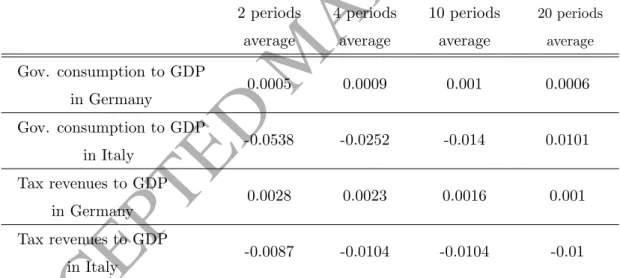
Second, we study an exogenous case in which fiscal variables in Italy and Germany mimic their values in the actual data between 2012 and 2015 (see e.g. EMU-Public Finances, 2015, p. 15, by the European Commission). In practice, any fiscal consolidation in Italy, during that period, was achieved by an increase in total tax revenues as share of GDP by around 2 percent-age points, while total public spending to GDP share remained more or less unchanged.26 At the same time, in Germany, fiscal policy was kept neutral meaning no changes. To implement this scenario, in our simulations, we appropriately adjust the feedback policy coefficients on

25_{The exact numerical value we use for steady stateβ}∗_{is not important to our main results. But we do need}

β∗=βto get a well-defined steady state solution to the extent that we do not have premia in this new steady state.

26_{In Italy, tax revenues as share of GDP were 45.6% in 2011 and this increased to 47.8% in 2012 and to 48.2%}

ACCEPTED MANUSCRIPT

public debt in the fiscal policy rules in the two countries, so as the generated values of fiscal variables (total tax revenues and public spending as shares of GDP) are close to those in the data during the first four years (namely, 2012-5) after departure from the status quo solution in Table 2. Thus, under this scenario, policy reaction is not chosen optimally; instead, the fiscal feedback policy coefficients are adjusted so as to mimic the actual policy in the period 2012-5. The monetary authority’s reaction to weighted inflation in the two countries, φ_π, is also set exogenously at, say, 2 (we report that results for this exogenous case are not sensitive to this value to the extent thatφ_π >1, which is the so-called Taylor principle). Further details and results of this ad hoc scenario are in subsection 5.2.

4.3

Optimized policy rules, solution methodology and welfare comparison

The single monetary authority can choose the feedback policy coefficients on inflation and output in the two countries in its single rule for the nominal interest rate (see equation 17 above), while each national fiscal authority can choose the feedback policy coefficients on national public debt and output in its rules for public spending and tax rates (see equations 18-22 above for each country).

We start with defining the welfare objective of policymakers.

4.3.1 Welfare objective of policymakers

There can be many institutional scenarios regarding the degree of cooperation between the single monetary authority and the two national fiscal authorities, ranging from full cooperation to zero cooperation. In this paper, we mainly focus on a scenario of full cooperation at policy level (however in section 7 below we also study Nash equilibria). Apart from computational simplicity, we focus on this scenario because, these days, most macroeconomic measures, and especially fiscal consolidation measures, are taken under the advice, or coordination, of the European Union and the ECB.

In particular, we assume that all monetary and fiscal feedback policy coefficients are chosen jointly and simultaneously so as to maximize a weighted average of households’ expected discounted lifetime utility in the two countries defined as:

Wt =ηVt+ (1−η)Vt∗ (30)

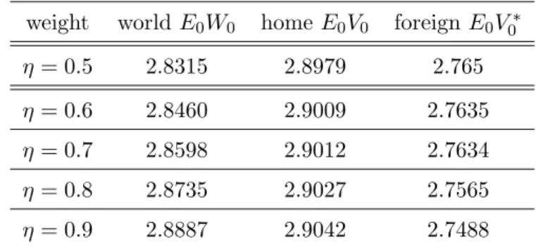
where 0≤ η ≤1 is the political weight of the domestic country vis-a-vis the foreign country, i.e. the higher is η, the higher the say of Germany in policy-making (see also equation (17) above), andVt andVt∗ are as defined in equation (7) above for each country. As said, we start

ACCEPTED MANUSCRIPT

with the neutral caseη= 0.5, but we will experiment with various values ofη in section 6.

4.3.2 Computation of optimized feedback policy rules

Except for the ad hoc scenario discussed in subsection 4.2, we compute the welfare-maximizing values of feedback policy coefficients in the policy rules (this is what Schmitt-Groh´e and Uribe, 2005 and 2007, call optimized policy rules). The welfare criterion is to maximize the conditional welfare of the two households as defined in (30) above, where conditionality refers to the initial conditions chosen; the latter are given by the status quo solution in Table 2 above, which is close to the data averages over 2001-2011. To this end, following Schmitt-Groh´e and Uribe (2004), we take a second-order approximation to both the equilibrium conditions and the welfare criterion.27 _{Specifically, we first compute a second-order approximation of both the conditional}

welfare and the decentralized equilbrium around the associated steady state, as functions of feedback policy coefficients using Dynare and, in turn, we use a matlab function (such as fminsearch.m) to compute the values of the feedback policy coefficients that maximize this approximate system (Dynare and matlab routines are available upon request). In this exercise, if necessary, the feedback policy coefficients are restricted to be within some prespecified ranges so as to deliver determinacy. All this is with, and without, debt consolidation, where the case without consolidation will serve as a benchmark.

Regarding the zero lower bound (ZLB) for the nominal interest rate, we work as in e.g. Schmitt-Groh´e and Uribe (2007), which means that, when necessary, we simply place addi-tional restrictions on the range of feedback policy coefficients in the Taylor rule, φ_π and φ_y in equation (17), so that the gross nominal interest rates do not violate the ZLB, in other words, Rt, Qt, Rt∗, Q∗t > 1. We report that only in the case of flexible exchange rates,

stud-ied in subsection 7.2 below, such additional restrictions will be required (details for this case are postponed until then). In all other cases, at least under the parameterizations used, the ZLB is not violated; the main reason seems to be that our initial conditions feature relatively high debt and relatively high nominal interest rates, which are, in turn, gradually reduced by optimally chosen debt consolidation policies in the transition.28

27_{We focus on second-order accurate approximate solutions because, when the model is stochastic, first-order}

approximations can give spurious results when used to compare the welfare under alternative policies (see e.g. the review in Gal´ı, 2008, pp. 110-111). We report that we have also experimented with non-approximate solutions in the deterministic case and the main results do not change.

28_{By contrast, the initial conditions in Erceg and Lind´e (2013) are consistent with a deep output contraction,}

produced by (among other things) a big adverse TFP shock, which, in combination with the assumed feedback policy coefficients, leads to sharp policy interest rate cuts in order to keep output near potential and inflation near target. In our paper, both in the baseline parameterization and in the sensitivity tests in sections 6 and 7, this possibility does not arise, except in the flexible exchange rate regime discussed below. For a methodology paper on the ZLB, see e.g. Fern´andez–Villaverde et al. (2015).