14
Universidade do Minho
José Alberto de Sousa Rodrigues
Modeling, mathematical and numerical
analysis of a vacuum breaker.
Implementation and numerical simulation
Escola de Ciências
José Alber
to de Sousa R
odrigues
Modeling, mat
hematical and numerical
anal ysis of a v acuum break er . Implement
Tese de Doutoramento em Ciências
Especialidade em Matemática
Trabalho realizado sob a orientação do
Professor Doutor Stéphane Louis Clain
Universidade do Minho
José Alberto de Sousa Rodrigues
Escola de Ciências
Modeling, mathematical and numerical
analysis of a vacuum breaker.
Acknowledgements
First and foremost, this thesis would not have been possible without the help and advice of my advisor, Prof. Dr. Stphane Clain. As much as I am indebted to him for all of the knowledge he conveyed to me, and for the time he generously spent with me, there is another thing I am most thankful for. I would also like to extend my thanks to Prof. Dr. Juan Via˜no Rey for his useful and constructive recommendations on mechanical problem resolution. Finally, I would like to thank wholeheartedly my family and give a very special thanks to my wife Isabel for her strong support and patience during my work on this thesis.
Braga, January 2014
Resumo
Esta disserta¸c˜ao tem como objetivo a modela¸c˜ao matem´atica, a an´alise do problema cont´ınuo, a discretiza¸c˜ao usando o m´etodo dos elementos finitos e a simula¸c˜ao num´erica implementada em C++, dum disjuntor de v´acuo de m´edia tens˜ao. Este ´e um problema multif´ısico envolvendo elasticidade n˜ao linear, para descrever a zona de contacto entre os el´etrodos, eletricidade, na avalia¸c˜ao da corrente que atravessa os el´etrodos de cobre, e eletromagnetismo, para avaliar a for¸ca repulsiva de Laplace.
O funcionamento dum disjuntor baseia-se num princ´ıpio muito simples, a saber: uma mola pressiona os el´etrodos um contra o outro, por forma a garan-tir um contacto el´etrico. A corrente que atravessa dum el´etrodo ao outro ´e determinada pela medida da zona de contacto e gera uma for¸ca de Laplace. Devido `as carater´ısticas geom´etricas dos el´etrodos, a for¸ca de Laplace tem sentidos opostos, em cada um dos el´etrodos, provocando assim uma for¸ca de repuls˜ao, conduzindo ao afastamento dos el´etrodos, interrompendo o circuito quando a intensidade atinge um valor cr´ıtico. Do ponto de vista t´ecnico, a posi¸c˜ao de equ´ılibrio e a zona de contacto resultam do importante equil´ıbrio estabelecido entre as for¸cas da mola e repulsiva de Laplace. Este equilib-rio resulta de dois subproblemas, nomeadamente: o problema mecˆanico e o problema eletromagn´etico. Consequentemente este trabalho foi dividido em trˆes partes, a saber:
Primeiro, a parte mecˆanica relativa `a a¸c˜ao da mola e da for¸ca vol´umica de Laplace, para determinar a medida final da zona de contacto. Aqui foi elab-orado o modelo matem´atico, estudadas as suas propriedades (existˆencia e unicidade de solu¸c˜ao) , estabelecida a discretiza¸c˜ao, usando o m´etodo de el-ementos finitos, e a correspondente implementa¸c˜ao com vista `a obten¸c˜ao de resultados num´ericos.
Na segunda parte tratamos o modelo do problema eletromagn´etico formu-lado em dois dom´ınios com uma fronteira comum. Nesta fase tratamos da existˆencia e unicidade de solu¸c˜ao, propomos uma discretiza¸c˜ao, usando o m´e todo dos elementos finitos, e fazemos a respectiva implementa¸c˜ao e simula¸c˜ao num´erica.
propomos um m´etodo de ponto fixo, para atingir a posi¸c˜ao de equil´ıbrio, justificando-o aos n´ıveis cont´ınuo e discreto. Esta parte ´e finalizada com simula¸c˜oes num´ericas relevantes do ponto de vista t´ecnico no contexto do problema eletromagn´etico.
Abstract
The PhD dissertation is dedicated to the mathematical modelling, the anal-ysis of the continuous problem, the discretization using the finite element method and the numerical simulation coding in C++ of a medium voltage vacuum circuit breaker. We have to face a multi-physics problem involving nonlinear elasticity to describe the electrodes and the contact zone, electric-ity to evaluate the current flowing across the copper bodies and electromag-netism problem to evaluate the repulsive Laplace force.
A circuit breaker is based on a simple principle. A spring presses down two copper bodies to maintain an electrical contact. The current flowing between the two electrodes is determined by the extension of the contact zone and generate Laplace force. Due to the geometrical characteristics of the elec-trodes, Laplace forces are opposite and create a repulsive force. When the intensity reaches a critical value, the forces separate the two electrodes and the circuit is breaking. From an engineering point of view, the equilibrium position and the contact area deriving from the balance between the spring constraint and the repulsive Laplace force is of critical importance.
Such an equilibrium results from two mathematical sub-problems, namely, the mechanical problem and the electromagnetic problem. In consequence, the work is constituted of three parts: the mechanical part concerns the ac-tion of the spring and the Laplace volumic force to determine the final contact area. We have elaborated the model, studied its mathematical properties (existence and uniqueness), designed numerical discretizations based on the finite element method and carried out an implementation of the method to achieve numerical simulations. The second part deals with the electromag-netic aspect where we propose a bi-domain model separated with a common interface. We prove existence and uniqueness of the model, propose a finite element discretisation and at last carry out an implementation with numer-ical simulations. The last part is dedicated to the global problem where we propose a fixe point method to reach the equilibrium states. We justify the iterative process both at the continuous and the discrete levels. We end the third part with some numerical simulations which are of interest in the engineering context of the electromechanic problem.
Contents
Acknowledgements i
Abstract i
List of Figures viii
List of Tables xi
The Vacuum circuit breaker 1
I
The mechanical problem
6
1 Mathematical modeling of the contact problem 7
1.1 Introduction . . . 7
1.2 Problem statement . . . 7
1.3 The constitutive Law . . . 10
1.4 Boundary conditions . . . 11
2 Existence and uniqueness for the mechanics problem 13 2.1 Introduction . . . 13
2.2 Functional spaces . . . 13
2.2.1 Trace spaces and properties . . . 14
2.2.2 Trace spaces for the contact boundaries . . . 15
2.2.3 Functional spaces for the contact problem . . . 16
2.3 Variational formulation . . . 16
2.4 Existence and uniquenes . . . 19
2.4.1 Some technical lemmas . . . 20
2.5 Lagrange multipliers formulation . . . 23
2.5.1 Trace operator for the stess tensor . . . 23
2.5.2 Lagragian multipliers and mixted formulation . . . 24
3 Discretisation of the mechanical problem 28
3.1 Mesh and notations . . . 28
3.2 Discretization . . . 31
3.2.1 Discrete variational space . . . 31
3.2.2 Interpolations and projections . . . 32
3.2.3 Operator discretizations . . . 34
3.3 The Uzawa method . . . 35
3.3.1 The discrete formulation . . . 35
3.3.2 Saddle point and minimizer . . . 35
3.3.3 Matricial expression . . . 36
3.3.3.1 Matricial version of the minimizing problem . 39 3.3.3.2 Matricial version of the saddle point problem 39 3.3.3.3 Active zone . . . 39
3.4 The Uzawa’s algorithm . . . 40
3.5 The discrete Haslinger method . . . 40
4 Numerical simulation 42 4.1 The problem to solve numerically . . . 42
4.2 Full contact case . . . 43
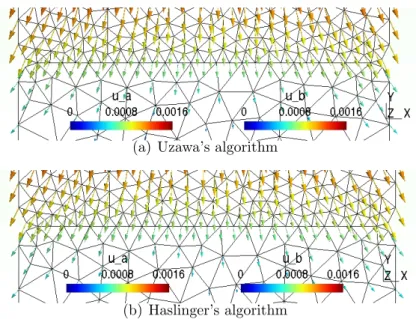
4.2.1 Algorithms comparison . . . 43
4.2.2 Algorithms performence . . . 44
4.2.3 Mortar space influence . . . 45
4.2.4 Mesh convergence . . . 46
4.3 Curve contact case . . . 49
4.3.1 First test: Elliptic profile and large deformation . . . . 49
4.3.2 Second test: Elliptic profile and small deformation . . . 52
4.3.3 Third test: Circular profile and large deformation . . . 54
4.3.4 Fourth test: Circular profile and small deformation . . 57
4.4 Active zone function . . . 59
II
The electrical problem
62
5 Mathematical modelling 63 5.1 The mapped domain . . . 645.2 The electrical problem . . . 64
5.2.1 The two domains formulation . . . 65
6 Existence and uniqueness for the electrical problem 68
6.1 Functional spaces and trace . . . 68
6.2 The two domains formulation . . . 70
6.2.1 Existence and uniqueness for φa . . . 70
6.2.2 Existence and uniqueness for φb . . . 71
6.3 The iterative procedure . . . 72
6.4 Existence and uniqueness for the magnetostatic problem . . . 73
6.4.1 Radial field at the infinity . . . 73
6.4.2 The Laplace force . . . 75
7 Discretization of the electric problem 76 7.1 Meshes and notations . . . 76
7.2 Discretization by finite element method . . . 77
7.2.1 Discrete variational space . . . 78
7.2.2 Operators . . . 80
7.2.3 The iterative procedure . . . 81
7.2.3.1 Existence and uniqueness for φah . . . 81
7.2.3.2 Existence and uniqueness for φbh . . . 81
7.2.3.3 The fixe point . . . 81
7.3 Matricial representation . . . 82
7.3.1 Representation for Aae h . . . 82
7.3.2 Representation for Abeh . . . 83
7.3.3 Current density and normal projection . . . 83
7.3.4 Representation for the mappings on I . . . 84
7.3.5 The iterative problem within the matricial form . . . . 84
8 Numerical simulation 86 8.1 One domain case . . . 86
8.2 Two domains case . . . 90
8.2.1 Elliptic profile . . . 90
8.3 Circular profile . . . 95
III
The global problem
98
9 Mathematical modelling 99 9.1 The continuous global problem . . . 999.1.1 The iterative algorithm . . . 99
9.1.2 Convergence of the iterative process . . . 100
9.2 The discrete global problem . . . 102
9.2.2 Analysis of the algorithm . . . 103
10 Numerical analysis of global problem 107
10.1 Circular profile . . . 107 10.2 Elliptic profile . . . 110
A Functional spaces 115
A.1 Lp spaces . . . 115 A.2 Sobolev spaces . . . 116
B Variational inequalities 120
B.1 Introduction . . . 120 B.2 Existence of a Solution . . . 121
List of Figures
1 The circuit-breaker [8] . . . 2
2 The circuit-breaker modelling: a coupling of three mathemat-ical sub-problems . . . 4
1.1 Outline of the circuit-breaker, each electrode has high ha = hb = 0.08 m and as base 0.2 m . . . 8
3.1 Regularity parameters for a triangle . . . 29
3.2 Outline for the discretizations procedure . . . 30
3.3 Global and local numeration nodes over Ξη . . . 31
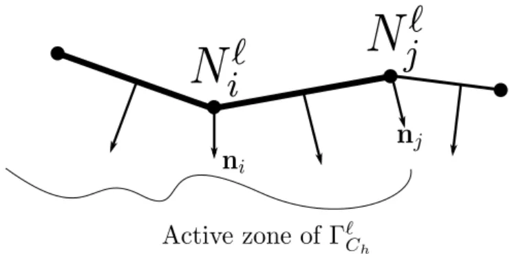
3.4 The normal at the node is the average of the normals of the adjacent sides . . . 38
3.5 Discrete active zone definition . . . 40
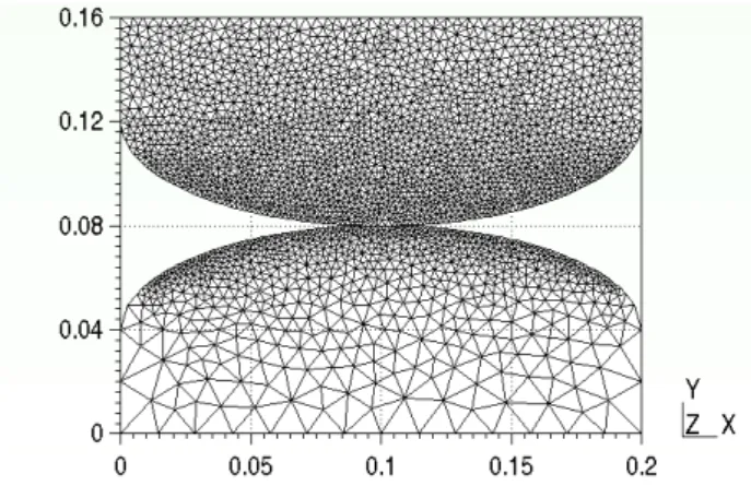
4.1 Initial circuit breaker’s shape and nonmatching mesh . . . 44
4.2 Displacement field with a coarse mesh . . . 44
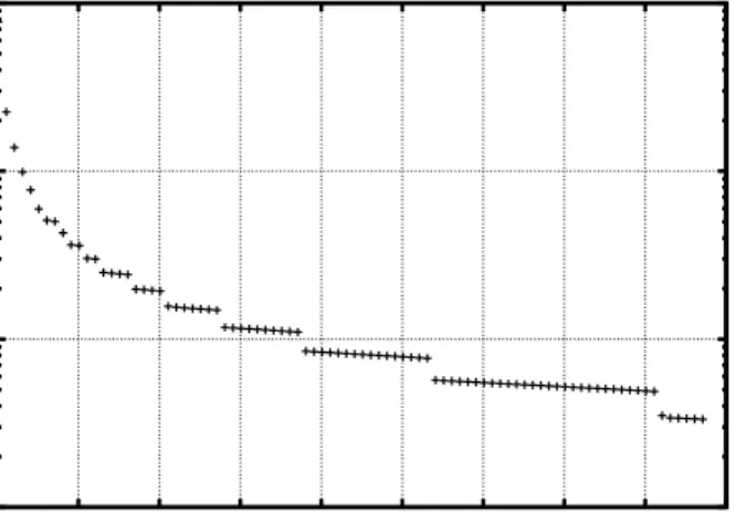
4.3 Zoom of displacement field at contact zone with a coarse mesh 45 4.4 Relative residue graph for a coarse mesh . . . 46
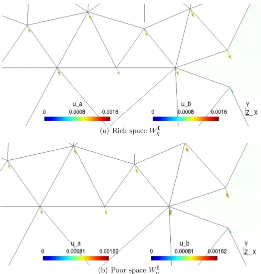
4.5 Displacement field obtained when WηI is poor . . . 46
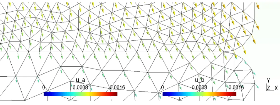
4.6 The fisplacement field is no more continuous at interface after a reduction of the dimension of discrete space WηI (Figure (b)) 47 4.7 Displacement field with a refined mesh . . . 48
4.8 Zoom of displacement field at contact zone with a refined mesh 48 4.9 Diagram of application of central spring force . . . 49
4.10 Elliptic profile: Initial circuit breaker’s shape and nonmatch-ing mesh . . . 50
4.11 Elliptic profile: Zoom of figure at the potential contact zone . 50 4.12 Elliptic profile: Zoom of displacement field for global applied spring force andα = 0.1, using Uzawa’s algorithm . . . 50
4.13 Elliptic profile: Zoom of deformed mesh at the contact zone with α= 0.1 . . . 51
4.14 Elliptic profile: Relative residue graph for α = 0.1, using
Uzawa’s algorithm . . . 51
4.15 Diagram of application of lateral spring force . . . 52
4.16 Elliptic profile: Zoom of displacement field at the contact zone 52 4.17 Elliptic profile: Zoom of deformed mesh at the contact zone with α= 0.01 . . . 53
4.18 Elliptic profile: Relative residue graph for α = 0.01, using Uzawa’s algorithm . . . 53
4.19 Circular profile: Initial circuit breaker’s shape and nonmatch-ing mesh for the third test . . . 55
4.20 Circular profile: Zoom of displacement field of figure at the contact zone . . . 55
4.21 Circular profile: Zoom of deformed mesh at the contact zone with α= 0.1 . . . 56
4.22 Circular profile: Relative residue evolution . . . 56
4.23 Circular profile: Zoom of displacement field at the contact zone . . . 57
4.24 Circular profile: Zoom of deformed mesh at the contact zone with α= 0.01 . . . 57
4.25 Circular profile: Relative residue graph for α = 0.01, using Uzawa’s algorithm . . . 58
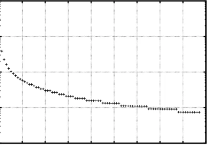
4.26 Elliptic profile: Evolution of the length of active zone ”×” and least squares aproximation ”line” . . . 60
4.27 Circular profile: Evolution of the length of active zone ”×” and least squares aproximation ”line” . . . 61
5.1 Electric-Magnetic problem outline . . . 64
8.1 Domain mesh . . . 87
8.2 Potential scalar field . . . 88
8.3 Current density field . . . 88
8.4 Zoom of current density field at contact zone . . . 89
8.5 Magnetic induction (componant followinge3 ) . . . 89
8.6 Laplace force . . . 89
8.7 Elliptic profile and large active zone: Repulsive force generated ”×” and least squares aproximation ”line” . . . 92
8.8 Elliptic profile and small active zone: Repulsive force gener-ated ”×” and least squares aproximation ”line” . . . 93
8.9 Elliptic profile: Evolution of relative the residue for electric problem resolution, with α = 0.1 and I = 10 kA andθ =.5 . . 93
8.10 Elliptic profile: Evolution of relative the residue for electric problem resolution, with α = 0.1 and I = 10 kA andθ =.25 . 94 8.11 Elliptic profile: Evolution of relative the residue for electric
problem resolution, with α = 0.1 and I = 10 kA andθ =.125 94 8.12 Circular profile and large active zone: Repulsive force
gener-ated ”×” and least squares aproximation ”line” . . . 96 8.13 Circular profile and small active zone: Repulsive force
gener-ated ”×” and least squares aproximation ”line” . . . 97 9.1 The four configurations . . . 104 10.1 Zoom of electrodes configuration at the contact zone for α =
0.1 andI0 = 100 kA with a circular profile . . . 108 10.2 Potencial and density field at equilibrium configuration for
α= 0.1 andI0 = 100 kA with a circular profile . . . 108 10.3 Zoom of electrodes configuration at the contact zone for α =
0.1 andI0 = 100 kA with a elliptic profile . . . 110 10.4 Potencial and density field at equilibrium configuration for
List of Tables
4.1 Performance of algorithms . . . 45
4.2 Elliptic profile: Results for a global spring force and α= 0.1 . 51 4.3 Elliptic profile: Results for a lateral spring force and α= 0.1 . 52 4.4 Elliptic profile: Results for a global spring force and α= 0.01 53 4.5 Elliptic profile: Results for a laterally spring force and α = 0.01 . . . 54
4.6 Circular profile: Results for a centred spring force andα = 0.1 56 4.7 Circular profile: Results for a lateral spring force and α= 0.1 57 4.8 Circular profile: Results for a lateral spring force and α= 0.01 58 4.9 Circular profile: Results for a laterally spring force and α = 0.01 . . . 58
4.10 Correspondence between the force and the active zone . . . . 59
4.11 Elliptic profile: Length of active zone . . . 60
4.12 Circular profile: Length of active zone . . . 61
8.1 Repulsive force generated with an elliptic profile and large active zone . . . 91
8.2 Repulsive force generated with an elliptic profile and small active zone . . . 92
8.3 Repulsive force generated with an circular profile and large active zone . . . 95
8.4 Repulsive force generated with an circular profile and small active zone . . . 96
10.1 Global results for a circular profile andI0 = 40 (kA) . . . 109
10.2 Global results for a circular profile andI0 = 60 (kA) . . . 109
10.3 Global results for a circular profile andI0 = 100 (kA) . . . 109
10.4 Global results for a circular profile andI0 = 60 (kA) . . . 111
The Vacuum circuit breaker
Circuit breaker and fuse are the two major apparatus involved in electrical power distributions and are subject to intensive studies and developments for two centuries. Charles Grafton (1836) and Thomas Edison (1879) were the pioneers of the circuit breaker conception but the first domestic circuit breakers only appear in the beginning of the 20th century (1935). High volt-age circuit breakers technology has changed radically in the past five decades regarded to the increasing demand and the necessary specialization. Most utility up-to-day systems are having mix population of bulk oil, minimum oil, vacuum, air blast, SF6 two-pressure, and SF6 single-pressure circuit break-ers. The SF6 single-pressure circuit breaker has become the current state of the art technology at transmission voltages (72.5 kV and above). However, SF6 gas has been identified as a greenhouse gas, and safety regulations are being introduced in many countries in order to prevent its release into the atmosphere.
Vacuum circuit breaker has emerged as the dominant technology in the medium voltage range due to its superior features such as long contact life, lack of maintenance requirement, low operating energy requirement and high reliability. In a vacuum circuit breaker, the electric interruption takes place in vacuum. This technology has been found to be most suitable for medium voltage application though the experimental interrupters for 72.5 kV and 145 kV have been developed.
Design of a vacuum interrupter
In principle, a vacuum interrupter has a steel arc chamber in the centre and symmetrically arranged ceramic insulators. Refer figure 1 showing the main parts of a typical vacuum interrupter.
2 4 5 8 6 7 1 9 2 3
Figure 1: The circuit-breaker [8]
We refer [8] and [12] to describe the interrupter: (1) a ceramic insulating envelope that is sealed at both ends by (2) metallic (stainless steel) plates brazed to the ceramic body so that a high vacuum container is created. The operating ambient pressure inside of the evacuated chamber of a vacuum in-terrupter is generally between 10−6 and 10−8torr (10−4−10−6 Pa). Attached to one of the end plates is the (3) stationary contact, while at the other end the (4) moving contact is attached to the bottle by means of (5) metallic spring. A metal vapor condensation shield (6) is located surrounding the set of contacts (7), either inside of the ceramic cylinder, or in series between two sections of the insulating container. The purpose of the shield is to provide a surface where the metal vapor condenses thus protecting the inside walls of the insulating cylinder so that they do not become conductive by virtue of the condensed metal vapor. A second shield (8) is used to protect the belows from the condensing vapor to avoid the possibility of mechanical damage. In some designs there is a third shield (9) that is located at the junction of the stationary contact and the end plate of the interrupter. The purpose of this shield is to reduce the dielectric stresses in this region.
Even though modern vacuum interrupter technology was developed in the early 1960s, it is still considered to be an evolving technology, as continuous improvements and innovations are taking place in this area. For example, the size and capability of modern vacuum interrupter bears no relationship to the one built in the 1960s. The diameter of the vacuum interrupter has been reduced from 20 cm in 1967 to 5 cm today. This size reduction is the result of major developments in vacuum technology, vacuum processing, con-tact material development and evolution of vacuum interrupter design. The contact geometry started from plain butt contacts in the 1960s and gradually progressed to spiral, cup and axial magnetic fields. The butt contact is the simplest, but is only suitable for interrupting the low current diffuse vacuum arc. It thus finds application in load break switches and contactors which are required to interrupt currents less than 4.5 kA. The transverse magnetic field contacts have spiral or skew slitted cup type construction. These contacts use the transverse magnetic field generated by the circuit current flowing in the spiral arms or skew slits of contacts to drive the high current, columnar, vacuum are rapidly over the contacts surfaces. This results in two effects: (a) the contact surface has uniform erosion and is left in a relatively smooth condition after high current arcing, and (b) the column cannot sustain itself when the current falls to current zero in an ac circuit. It thus returns to the diffuse mode, which is easily interrupted at current zero.
Circuit breaker principle
A vacuum circuit breaker is a device that allows the cutting of electrical power. The apparatus core is essentially constituted of two electrodes, one of them being mobile and subject to a mechanical force produced by a spring, maintaining the contact between the two electrodes. The current passing between two electrodes is determined by the extension of the contact zone and generated Laplace forces in areas bordering the contact, but not yet in contact. Due to the curved geometry of the electrodes, Laplace forces are opposite and cause the repulsion of the electrodes. When the intensity reach a critical value, the forces separate the two electrodes and the circuit is breaking. For a given intensity, the equilibrium position and the contact area result from the balance between the spring constraint and the repulsive Laplace deriving from the electric and magnetic fields.
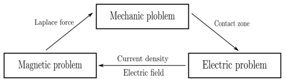
To determine the equilibrium, we have to consider three sub-problems, namely, the mechanical problem, the electrical problem and the magnetic problem. Indeed (see diagram in figure 2), the spring force in conjunction with the Laplace force determine the displacement of the two bodies and the contact
Figure 2: The circuit-breaker modelling: a coupling of three mathematical sub-problems
area. From the contact area, we deduce the current density distribution and the electric field. With the current density, we compute the magnetic field and we deduce the Laplace force with the electric and the magnetic field.
Outline of the Thesis
The thesis dissertation is divided in three parts: the first one deals with the mechanical aspect of the problem while we address the electromagnetic issues in the second part. The last part concerns the global problem linking the two sub-problems
• Chapter 1 introduces the mechanical and proposes a modelling of the contact problem.
• We address the question of existence and uniqueness for the two bod-ies contact problem in chapter 2 using the classical framework of the Hilbert spaces.
• The discretization is carried out in chapter 3 using the finite element method and a Mortar-like method. We also introduce an intermediate space to handle the contact zone. Code has been developed, imple-mented inC++and numerical simulations have been performed to prove the efficiency of the approach.
• The mathematical modelling of the electromagnetic problem is pre-sented in chapter 5 where we introduce a specific technique to take the contact zone into account.
• Existence and uniqueness of a solution for the electrical problem is given in chapter 6 using the Hilbert space H1+s,s∈[0,1/2[ to recover some regularity.
• The discretization of the electric problem is proposed in chapter 7 and a iterative algorithm is introduced and analysed.
• Implementation of a C++ and numerical simulation are carried out in chapter 8 to check the validity of the approach.
• We consider the global mathematical modelling in chapter 9 and in-troduce a fixe point method to solve the problem. Some mathematical results are given to justify our approach.
• Code implementation in C++ and numerical simulations are performed based on the fixe point methodology in chapter 10 to prove that nu-merically the algorithm converges and effectively provides a correct numerical approximation.
All the codes have been developed and implemented by the author using the Object Finite Element LIbrary OFELI of Pr. Touzani [20].
Part I
Chapter 1
Mathematical modeling of the
contact problem
1.1
Introduction
In functional regime, the two electrodes remain in contact to allow the electri-cal power delivery accross the common interface. The contact shape results from the initial electrodes shape (namely the curvature), the spring pres-sure and the Laplace force deriving from the current intensity. The present chapter is dedicated to the modeling of the contact problem between the two electrodes submitted to the spring force and a given volume force. The fun-damental point is the determination of the unknown contact shape based on the linear mechanic model due to the small electrode deformations involved in the circuit breaker problem.
After a short presentation of the mechanical problem, we propose a con-struction on the mathematical modeling based on the traditional signorini problem and derive several sub-model in function of the boundary condition.
1.2
Problem statement
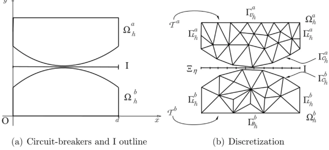
We consider a simplified but representative geometry of the circuit breaker apparatus constituted of two electrodes in contact, as in figure 1.
We denote by Ω = Ωa∪Ωbthe whole domain constituted of the two electrodes of same width d while Γa=∂Ωa and Γb =∂Ωb stand for the boundary. The bottom one is constituted by a hb height piece of copper named Ωb fixed on a support foundation denoted by ΓB, the interface between the electrode and
its support. The lateral sides of the electrode Ωb (denoted by ΓbL) is assumed to be free of constraint.
x y Spring
Ω
b
Ω
a
ΓaL ΓbC ΓbL ΓbL ΓaL ΓaC ΓB ΓUFigure 1.1: Outline of the circuit-breaker, each electrode has high ha =hb =
0.08 m and as base 0.2 m
A second upper electrode, characterized by a ha height domain Ωa is main-tained in contact with Ωb by applying a force on the upper side ΓU of Ωa.
We assume that the spring force is uniformly applied on the a subdomain of ΓU while ΓaL stands for the lateral side.
To close the boundary partition
Γa = ΓU ∪ΓaL∪Γ a C, Γb = ΓB∪ΓbL∪Γ b C. (1.1) ΓaC and ΓbC represents the two facing potential contact surface of Ωa and Ωb respectively. In the present study, we assume that the shape is an arc of cir-cle of respective radius Ra and Rb. At last, n` is the outward normal vector and t` the tangential vector such that t`,n` is a positive oriented basis of Ω`, `= 1,2.
Since the contact boundary will play a fundamental role, we have introduced a parametrization of each interface which allows to compare and realizes arithmetic operations between a function on ΓaC and an other function on ΓbC. We consider as the reference position the initial situation where the
two bodies are not submitted to any constraint (see fig 1.1 ) with contact boundary facing with only one point contact.
We assume a C2 class parametrization of the two boundaries χχχa and χχχb
defined on the parameter intervalI= [0, d] by the following one-to-one func-tions χ χ χa :I → ΓaC; χχχb :I → ΓbC; ξ 7→ χχχa(ξ)=(χa 1(ξ),χa2(ξ)); ξ 7→ χχχ b (ξ)=(χb 1(ξ),χb2(ξ)). (1.2) Let us now consider the situation when we apply the spring force and the body force. Domain Ωa and Ωb change to a new configuration which we characterized by the displacement vector
x∈Ω→u(x) = (u1(x), u2(x)),
wherexcorresponds to the position at the initial configuration and we adopt the notationua =u|Ωa andu
b =u
|Ωb for the restrictions on the subdomains.
Due to the displacement, interface ΓaC and ΓbC move and an effective contact zone (the active set) A ⊂ R2. Let define J⊂Isuch that
χχχa(ξ) +u(χχχa(ξ)) =χχχb(ξ) +u χχχb(ξ). (1.3) then one has
A={χχχa(ξ) +u(χχχa(ξ)), ξ∈J}. (1.4) To simplify the model taking into account that the radii are larger thandwe introduce parameter ε = max( d
Ra,
d
Rb) and notice that the maps defined in
(1.2) satisfy: ∂χχχa 1 ∂ξ = 1 ∂χχχb 1 ∂ξ = 1 ∂χχχa 2 ∂ξ =O(ε) ∂χχχb 2 ∂ξ =O(ε) . (1.5)
In pratice The electrode have a small diameter (d∈[0.2,0.8] in meter) with respect to the interface radii (around 100m). With such an assumption, the outward normal vector on ΓaC and ΓbC can be considered as colinear to the
Ox2 axe, in the following sense
na = 0 −1 ≈n(χχχa(ξ)) = O(ε) −1 ,nb = 0 1 ≈n χχχb(ξ)= O(ε) 1 .
Moreover, we shall assume that the interface displacements are perpendic-ularly that if y = (y1, y2) is a contact point of the new configuration, it corresponds to a pointxa = (xa1, xa2)∈ΓaC and a point xb = xb1, xb2∈ΓbC of the initial configuration such that xa1 =xb1 =y1.
Taking the inner product between relation (1.3) and n(χχχa), we have at any contact point
u χχχb(ξ)−u(χχχa(ξ))n χχχb(ξ)=g(ξ), (1.6) where g ∈C1(I), defined on I by
g(ξ) = χχχa(ξ)−χχχb(ξ)n χχχb(ξ)≥0, (1.7) is the gap between the two electrodes.
1.3
The constitutive Law
We now introduce the equations which govern the displacement. We assume that the two bodies are elastic and we denote by εεε(u) the strain tensor for any displacement u(x) with respect to x ∈ Ω in the initial configuration. The conservation of the impulsion reads
−divσσσ(u) =f in ΩΩΩ
where f represents the body force. In our case, f will be constituted by the gravity and the Laplace forces.
We denote byσσσ(u) the stress tensor and using the classical elasticity frame-work we consider an isotropic linear material where we state the Hooke’s law:
σ
σσ(u) = (λtr(εεε(u))I+ 2µεεε(u)), (1.8) where I denotes the 2-identity matrix, and
εεε= ε11= ∂u1 ∂x1 ε12 = 1 2 ∂u1 ∂x2 +∂u2 ∂x1 ε21= 1 2 ∂u2 ∂x1 + ∂u1 ∂x2 ε22 = ∂u2 ∂x2 (1.9)
is the strain tensor of the displacement vectoruandtr(·) represents the trace of a matrix. The Lam´e positive constants λ and µare given by
µ= E
2(1 +ν) and λ =
Eν
(1 +ν)(1−2ν),
1.4
Boundary conditions
We now prescribe the boundary conditions, beginning by those without con-tact:
• At the lateral sides Γaand Γb, no force and displacement are prescribed so we stateσσσn= 0 , on ΓaL∪ΓbL.
• The bottom part of the electrode is fixed so we required that no dis-placement occur and we state u= 0 on ΓB.
• The upper part is controlled by the spring and the normal force is governed by
nTσσσn=−κ(u·n+α)
where −κα is the initial force applied to the electrode while−κ(u·n) represents the force due to the displacement .
• Moreover we require that no lateral movement takes place, so we state u·t=0 on ΓU to prevent the horizontal movement.
Now we deal with the contact interface condition. For a given configuration (spring and body force ) the interfaces ΓaC and ΓbC move and we obtain two new interfaces eΓaC and ΓebC which are partially in contact (cf (1.4))
A=eΓaC∩ΓeaC. (1.10)
Using identities (1.5) - (1.7), the active set is implicitly defined as an interval J, such that for anyξ ∈J .
h u χχχb(ξ)−u(χχχa(ξ)) i n χχχb(ξ)=g(ξ) n(χχχa(ξ))Tσσσ u(χχχa(ξ)) n(χχχa(ξ)) = n χχχb(ξ)Tσσσ u χχχb(ξ) n χχχb(ξ) <0 t(χχχa(ξ))Tσσσ u(χχχa(ξ)) n(χχχa(ξ)) = t χχχb(ξ)Tσσσ u χχχb(ξ) n χχχb(ξ)=0. (1.11)
have: h u χχχb(ξ)−u(χχχa(ξ)) i ·n χχχb(ξ) < g(ξ) σ σσ u(χχχa(ξ)) n(χχχa(ξ)) =σσσ u χχχb(ξ) n χχχb(ξ) = 000. (1.12)
Note that the contact boundary is unknown , andJhas to be also determined. To sum up, the displacement functionusatisfies the following set of equations
−divσσσ(u) =f in Ω (1.13)
σσσ n = 000 on ΓaL∪ΓbL (1.14)
u = 000 on ΓB (1.15)
u·t = 0 on ΓU (1.16)
nTσσσ n =−κ(ua·n+α) on ΓUa with α ∈Rand κ >0 (1.17)
Chapter 2
Existence and uniqueness for
the mechanics problem
2.1
Introduction
The chapter is dedicated to the theoretical aspects of the problem. We first build the weak formulation of the problem and define the associated operator. Then we prove existence and uniqueness of the solution using the classical elasticity framework for contact problem as proposed in [13]. We point out three particularities of the problem we address: on the one hand we use a Robin like condition to model the spring action to maintain the electrodes in contact. On the other hand, the active zone is ana priori unknown of the problem since it depend of the spring force and the Laplace force generated by the current and its evaluation is of crucial importance for the global circuit breaker problem since it characterizes the conductivity area. At last we do not use the classical master-slave technique where we project one side of the domain (slave) to the other side (master) but we introduce an intermediate domain where the both potential contact boundary are projected, applying in some sense the idea of the three fields formulation [5].
2.2
Functional spaces
Notations and definitions of the generic functional spaces such as L2, H1
are given in Appendix A for the sake of consistency but specific functional spaces, linear and bilinear forms have to be introduced to prove existence and uniqueness of the solution.
2.2.1
Trace spaces and properties
We first recall some classical functional spaces and trace operator for a Lip-schitz domain. Let Ω be a open bounded domain such that the boundary
∂Ω is continuous lipschitz (see [13] p. 14). Functional space H12(∂Ω)
cor-responds to the scalar value Hilbert trace space associated to H1(Ω) while
H−12(∂Ω) = H 1
2(∂Ω)0 stands fot the dual space. We recall that the trace
operator
H1(Ω) → H12(∂Ω)
φ → γ0φ=φ|∂Ω is a linear bounded surjective application.
Since we also deal with vectorial value space, we setH1(Ω) =H1(Ω)×H1(Ω) and define L2(Ω) andH12(∂Ω) in the same way such that the trace operator u →γ0uis a bounded linear surjective operator from H1(Ω) ontoH
1 2(∂Ω).
For a lipschitz domain Ω, outward unit normal vector n is well-defined (see [13] p. 86) and we define the normal trace and tangential trace operetor with
H1(Ω)→ H12(∂Ω) H1(Ω) →H
1 2(∂Ω)
u→ γnu = (γ0u)·n u →γtu=γ0u−(γnu)n.
We recall the definition of the tangential trace space H 1 2 t(∂Ω) ={v ∈H 1 2(∂Ω); γnv = 0 on∂Ω}
then the operator
H1(Ω) → H12(∂Ω)×H
1 2
T(∂Ω)
u → (γnu, γtu)
is a linear bounded surjective operator (see [13] p. 87). Lettbe the tangential vector such that (t,n) is a positive oriented basis. Since γtu = (γTu).t =
(γ0u).t, we have
H1(Ω) →H12(∂Ω)
u →(γnu, γtu)
which is also a linear bounded surjective operator.
Let D⊂∂Ω be an open subset and set Σ =∂Ω\D. We introduce the trace space for a part of the boundary where a homogenous dirichlet condition is prescribed on the complementary part. To this end, we introduce
H 1 2 00(Σ) = γ0φ|Σ; φ∈H1(Ω), γ0φ|D = 0 = n η∈H12(Σ);d− 1 2(x, D)η∈L2(Σ) o
where d(x, D) is the distance between point xand set D. We recall that {φ∈H1(Ω);γ0φ|D = 0} → H 1 2 00(Σ) φ → γ0φ|Σ
is a linear bounded surjective operator. Note that for any open Σ0 ⊂Σ such that Σ0 ⊂Σ we have H12(Σ0) ={η| Σ0; η∈H 1 2 00(Σ)}={η|Σ0; η∈H 1 2(∂Ω)}.
2.2.2
Trace spaces for the contact boundaries
We recall that the full domain is composed of two subdomains Ω` with boundary Γ`, ` = a, b. Sets H1/2(Γ`C) = {φ|Γ`
C, φ ∈ H
1/2
(Γ`)} stand for the trace space on the respective contact boundaries Γ`C, ` = a, b and
H−1/2(Γ`C) = H1/2(Γ`C)0 correspond to the respective dual spaces. In the same way, H1/2(I) and H−1/2(I) = (H1/2(I))0 are the analogous functional spaces for the open interval I =]0, d[.
We introduce the trace operators on the contact boundaries setting
H1(Ω`) → H12(Γ`
C)
v → γn`v = (γnv)|Γ`
C.
It is a linear bounded surjective operator so there exist constantsα` >0 such that sup kvkH1(Ω`)=1 [q, γ0`v]≥α`kqk H−12(Γ` C)
where [·,·] stands for the duality pairingH−12(Γ`
C), H
1 2(Γ`
C).
Since χχχ` is a C2 one-to-one function from I onto Γ`C, we deduce that for any function φ ∈ H1/2(ΓC` ), φ ◦χχχ` ∈ H1/2(I) and φ → C`(φ) = φ ◦χχχ`
is a continuous isomorphism from H1/2(Γ`C) onto H1/2(I). It results that operators
H1(Ω`) → H12(I)
v → γI`v=γn`v◦χχχ`
are linear, bounded surjective applications and enjoy the inf-sup condition sup kvkH1(Ω`)=1 [q, γI`v]≥αe`kqk H−12(Γ` C) , (2.1) where αe` >0.
2.2.3
Functional spaces for the contact problem
We now turn to the specific functional spaces we need to prove existence and uniqueness of the contact problem. The Dirichlet condition u = 000 imposed on the boundary ΓB brings us to introduce the space Vb defined by
Vb =v = (v1, v2)∈H1(Ωb)|γ0v = 000 on ΓB . (2.2)
On the other hand, to impose the non lateral displacements on ΓU (1.16) we
introduce the functional space Va defined by:
Va =v = (v1, v2)∈H1(Ωa)2 |vt=γtv = 0 on ΓU (2.3)
and we define the set of admissible deformations by V =Va×Vb,
equipped with the norm
kvk2V = kv|Ωak21,Ωa+kv|Ωbk21,Ωb (2.4)
= kv1ak2H1(Ωa)+kva2k2H1(Ωa)+kv1bk2H1(Ωb)+kv2bk2H1(Ωb).
Since non negative functions on H1/2(I) correspond to a closed cone and define an ordening≥, for any function g ∈H1/2(I), we introduce the convex set K= n v ∈V| γIav+γIbv−g ≤0 in H12(I) o . (2.5)
From property (2.1) we deduce that K is closed. Indeed surjectivity yields that there exists w∈V such thatγIav+γIbv =g hence definition ofKturns to be K=v ∈V| γIa(v−w) +γIb(v−w)≤0 which is a closed set due the trace operators continuity.
2.3
Variational formulation
In this section, we aim to formally establish the weak formulation from sys-tem (1.13)-(1.17) and rewrite the problem as a minimization where we shall determine the energy functional.
Assumingu is a regular solution of problem (1.13)-(1.17) and letv be a test function. Multiplying relation (1.13) with v−u (inner product) integrating over domain Ω yields
− Z Ω divσσσ·(v−u)dx = Z Ω f ·(v−u)dx
Integration by parts gives (using the Enstein notation) Z Ω σ σ σij∂j(vi−ui)dx = Z Ω fi(vi−ui)dx+ Z ∂Ω σ σ σijnj(vi−ui)ds = Z Ω fi(vi−ui)dx+ Z ΓU σσσijnj(vi−ui)ds+ Z Γa C σσσijnj(vi−ui)ds+ Z Γb C σσσijnj(vi−ui)ds
where we have used the properties Z Γa L σ σ σijnj(vi−ui)ds = Z Γb L σ σσijnj(vi−ui)ds = Z ΓB σ σσijnj(vi−ui)ds = 0
We first deals with boundary ΓU. Regarding that (v−u)·t = 0, we have
(v−u) = [(v−u)·n]non ΓU and one writes
σ σσijnj(vi−ui) = σσσijnj[(v−u)·n]ni = niσσσijnj[(v−u)·n] = −κ(u·n+a) [(v−u)·n] which gives Z ΓU σσσijnj(vi−ui)ds = − Z ΓU κ(u·n+a) [(v−u)·n]ds.
Using the mappings from I onto ΓaC and onto ΓbC, we have Z Γa C σσσij(u)nj(vi−ui)ds = Z I σ σσij(u(χχχa))nj(χχχa)(vi(χχχa)−ui(χχχa)) dχdξχχadξ, Z ΓbC σσσij(u)nj(vi−ui)ds = Z I σ σσij(u(χχχb))nj(χχχb)(vi(χχχb)−ui(χχχb)) dχdξχχbdξ.
From the identity (1.5) we deduce
n(χχχa) = −n(χχχb) +O(ε), dχχχ a dξ ≈dχχχb dξ ≈1 +O(ε). (2.6) Since we assume the electrode has a small curvature ε with respect to the global dimension of the electrode we cancel the high-order terms in ε and
obtain Z Γa C σσσij(u)nj(vi−ui)ds+ Z Γb C σσσij(u)nj(vi−ui)ds = Z I σ σ σij(u(χχχa))nj(χχχa) vi(χχχa)−ui(χχχa) dξ+ Z I σ σ σij(u(χχχb))nj(χχχb) vi(χχχb)−ui(χχχb) dξ.
Since we assume a null tangential force tTσσσn= 0, the following relation for the stress tensor on Γ`C holds:
σ σ
σn = tTσσσnt+ nTσσσnn = nTσσσnn.
On the other hand, relations (1.11) and (1.12) yields the continuity of the normal stress nTσσσn or a null normal stress tensor hence we have
A = σσσ(u(χχχa))n(χχχa)· v(χχχa)−u(χχχa)+σσσ(u(χχχb))n(χχχb)· v(χχχb)−u(χχχb) = {nT(χχχb)σσσ(u(χχχa))n(χχχb)}n(χχχb)· u(χχχa)−v(χχχa)+
{nT(χχχb)σσσ(u(χχχa))n(χχχb)}n(χχχb)· v(χχχb)−u(χχχb)
= {nT(χχχb)σσσ(u(χχχa))n(χχχb)}n(χχχb)·(v(χχχb)−v(χχχa))−(u(χχχb)−u(χχχa)).
The contact condition (1.11) and (1.12) implies
A={nT(χχχb)σσσ(u(χχχa))n(χχχb)}n(χχχb)·(v(χχχb)−v(χχχa))−g
since either nT(χχχb)σσσ(u(χχχa))n(χχχb) = 0 outside of the active zone or either n(χχχb)· u(χχχb)−u(χχχa) =g on the active zone.
Taking into account that v ∈K, we have
nT(χχχb)σσσ(u(χχχa))n(χχχb)≤0, n(χχχb)· v(χχχb)−v(χχχa))≤g
we deduce that A≥0 and consequently Z Γa C σ σσij(u)nj(vi−ui)ds+ Z Γb C σ σσij(u)nj(vi−ui)ds≥0.
We then obtain the variational inequality Z Ω σ σσij∂j(vi−ui)dx ≥ Z Ω fi(vi−ui)dx− Z ΓU κ(u·n+α) [(v−u)·n]ds or equivalently Z Ω σσσ :εεε(v−u)dx+ Z ΓU κu·n[(v−u)·n]ds≥ Z Ω f·(v−u)dx− Z ΓU κα[(v−u)·n]ds (2.7)
2.4
Existence and uniquenes
Let u,v ∈V , we introduce the following bilinear forms
Aam(u,v) = Z Ωa σσσ(u) :εεε(v)dx+ Z ΓU κ(u·n)(v·n)dσ, (2.8) Abm(u,v) = Z Ωb σσσ(u) :εεε(v)dx, (2.9) Am(u,v) = Aam(u,v) +A b m(u,v), (2.10)
and linear forms:
Lam(v) = Z Ωa f ·vdx+ Z ΓU καw·nds, (2.11) Lbm(v) = Z Ωb f ·vdx, (2.12) Lm(v) = La(v) +Lb(v). (2.13)
From the variational inequality (2.7) we introduce the Signorini’s problem:
Findu ∈K such that
Am(u,v−u) ≥ Lm(v−u),∀v∈K.
(2.14)
The variational inequality problem turns to be a constrained minimization problem setting F(v) = 1
2Am(v,v)−Lm(v):
find u∈K such that
F(u) ≤ F(v),∀v∈K.
(2.15)
We recall here the main result (Theorem 3.9 in [13] p. 41)
Theorem 2.4.1 IfAm is a bilinear form which satisfies condition (3.14) and
L is a linear form which satisfie condition (3.15)of [13] p.38 then problem (2.15) admits a unique solution u ∈ V. Moreover u is the unique solution of the variational inequality problem (2.14).
Properties for operator Bv = γIav +γIbv have been checked, in particular the surjectivity. As we shall se in the next subsection, continuity of oper-ators Am(u,v) and Lm(v) derived from the cauchy-schwarz inequality with
Remark 2.4.1 In fact, the surjectivities of γIa and γIb are not strictly nec-essary. Indeed, the point is that K must be a non-empty closed convex set. Convexity derived from that the inequality is preserved by convex combina-tion while the set is close due to the continuity of trace operators. Surjectivity is used in general to ensure that K is not empty but in our case, the non-negativity of g yields that v = 0 belongs to K. So, at that stage, surjectivity is no longer required.
2.4.1
Some technical lemmas
We first report some classical results and refer [6] for detailed
Lemma 2.4.1 The form bilinear defined by (2.9) is continuous and coercive on Vb
Abm(u,v) ≤ c2kukVbkvkVb, (2.16)
Abm(u,u) > α2kuk2Vb, (2.17)
for all u,v∈Vb.
Proof: The continuity derives from the Cauchy-Schwarz inequality in L2.
Thanks to the homogeneous Dirichlet condition on ΓB, the Poincar´e
inequal-ity holds hence the semi-norm and the normVbare equivalent. The coercivity then derives immediatly from standard arguments (see [6]).
The situation for the bilinear form Aam is more complex.
Lemma 2.4.2 The form bilinear defined by (2.8) is continuous and coercive on Va
Aam(u,v) ≤ c1kukVakvkVa (2.18)
Aam(u,u) > α1kuk2Va (2.19)
for all v,w ∈Va.
Proof: As in the previous lemma, the continuity derives from the
Cauchy-Schwarz inequality in L2. Since no homogeneous condition are prescribed on a part of the boundary, Poincar´e inequality does not hold any longer. However the spring condition (1.17) will provide the coercivity. To this end, we assume that the coercivity of the form Aam does not hold on Va and show that such assumption is not compatible with the spring condition. If coercivity no longer hold then
Taking ε= 1 k, k∈N, there exists uk∈V a such that Aam(uk,uk)< 1 kkukk 2 Va.
We introduce the normalized vector wk =
uk kukkVa and we get a wk ∈ Va such that kwkkVa = 1, Aam(wk,wk)< 1 k. (2.21)
The sequence (wk) is bounded in Va which the bounded balls are compact
subsets of L2(Ωa). We deduce that there exists a subsequence (still denoted by (wk)k∈N) such that wk k →w inL2(Ωa) and wk k *w weakly inH1(Ωa),
with w ∈Va. We first deduce from (2.21)
Aam(wk,wk) k
→0. (2.22)
On the other hand we can write
Aam(wk,wk) = Z Ωa σ σ σ(wk) :εεε(wk)dx+ Z ΓU κ(wk·n)2dσ = Z Ωa εεε(wk) :εεε(wk) + div(wk)div(wk)dx + Z ΓU1 κ(wk·n)2dσ ≥ C Z Ωa εεε(u) :εεε(v) + Z ΓU κ(wk·n)2dσ ≥ C|wk|1,Ωa+ Z ΓU κ(wk·n)2dσ.
From relation (2.22) we deduce
|wk|1,Ωa + Z ΓU k(wk·n)2dσ k →0.
Since |wk|1,Ωa →k 0 andwk *k w in H1(Ωa), we have for anyϕϕϕ∈(D(Ωa))2
Z Ωa ∂xiwk·ϕϕϕdx k → Z Ωa ∂xiw·ϕϕϕdx
and the Cauchy-Schwarz inequality gives Z Ωa ∂xiwk·ϕϕϕdx ≤ |∂xiwk|0,Ωa|ϕϕϕ|0,Ωa ≤ |ϕϕϕ|0,Ωa|wk|1,Ωa k →0 Consequently, we have Z Ωa ∂xiwk·ϕϕϕdx k → 0, hence Z Ωa ∂xiw·ϕϕϕdx = 0, ∀ϕϕϕ ∈(D(Ω a))2 which implies |w|1,Ωa = 0
Since ∂xiw= 0, i= 1,2, the function is constant in Ω
a. Moreover we deduce
that ∂xiwk strongly converge to ∂xiw in L
2
(Ωa),i= 1,2. With wk strongly
converging to w in L2(Ωa) we conclude that
kwk−wk1,Ωa k
→0.
From relation (2.22) we have Z
ΓU
(γnwk)2 k
→0.
Regarding Yosida [23], the strong convergence wk k → w in H1(Ωa) implies γ0(wk) k →γ0(wk) on H1/2(ΓU) henceγnwk k →γnw so that γnw = 0 on ΓU.
On the other hand,w ∈Va yields with condition (1.16) that for any x∈ΓU
γ0w= (γnw)n+ (γtw)t = (γtw)t= 0
and we conclude γ0w = 000 on ΓU, hence w = 000 on Ωa. This last conclusion
brings a contradiction with the initial assumption (2.20) and (2.21), since we have
kwkk1,Ωa →k 16=kwk1,Ωa = 0.
Consequently Aam(·,·) is coercive in Va.
Coercivity of operator Am derives from lemmas 2.4.1 and 2.4.2 and we have
the following theorem.
Theorem 2.4.2 Let f ∈ V0. Then there exists a unique solution u in V
2.5
Lagrange multipliers formulation
2.5.1
Trace operator for the stess tensor
Assuming that f ∈ L2(Ω), it is proven in [13] pp.91–93 that the Green’s formula holds and trace operator σσσn on ∂Ω is defined. Indeed, let T =
{σσσ; σσσij ∈L2(Ω) and ∇.σσσ ∈L2(Ω)}, there exists a bounded linear operator
T → H−12(∂Ω)
σ σ
σ → π(σσσ) =σσσ n|∂Ω
such that for any v ∈H1(Ω), the Green’s formula holds Z Ω σ σσij∂xjvi = Z Ω ∂xiσσσijvj+< π(σσσ), γ(v)>H−12(∂Ω),H12(∂Ω) .
Moreover, we can define πn(σσσ) = π(σσσ)·n and πt(σσσ) = π(σσσ).t in H−
1 2(∂Ω)
such that π(σσσ) = πn(σσσ)n+πt(σσσ)t which are a generalization of the
classi-cal traces ntσσσn and tσσσn for continuous tensors. From a practical of view, such operators define the normal and tangential pressure (or traction) on the boundary.
Extension for a open subset Σ ⊂∂Ω can be considering. Assuming W ={u∈H1(Ω); γ0u= 0 on D}
then on can define a unique mappingπ|Σ fromT into H
1 2
00(Σ)
0
which is the closure of the trace operator
σ
σσ→(σσσijnj)|Σ such that we have
Z Ω σ σσij,jvjdx+ Z Ω σ σσijvi,jdx= Z Σ π|Σσσσ·γ|Σvds.
At last, if Σ0 is an open part of the boundary such that Σ0 ⊂ Σ then there exists a unique trace operator π|Σ0 such that πΣ0σσσ ∈H−
1 2(Σ0).
Returning to our specific problem we have the following theorem
Theorem 2.5.1 Let f ∈ L2(Ω) and u∈ V the solution of (2.14). Then u
is the solution of (1.13)-(1.17).
Proof: Since assuming that ∇ ·σσσ = f ∈ L2(Ω) trace operators π|Γa C and
π|Γb
C are well-defined on the contact boundaries and for anyσσσand the Green’s
formula holds which implies that u is a solution of (1.13)-(1.17) in a weak
2.5.2
Lagragian multipliers and mixted formulation
We now provide a new formulation based on the Lagrangian multipliers. We introduce the following linear operators
T →H−12(I), T →H− 1 2(I), πaIσσσ(t) = π|Γa Cσσσ·n a◦χχχa(t), πb Iσσσ(t) = π|Γb Cσσσ·n b◦χχχb(t),
which correspond to the normal pressure of the stress tensor of both side, using the representation on intervalle I.
Since solution u∈K withσσσ∈ T, we have for any function v∈K
Z Ω σ σσij∂jvidx+κ Z ΓU (u·n)(v·n)ds = Z Ω f ·vdx−ακ Z ΓU v·nds+ Z I πIa(σσσ)γIa(v)dt+ Z I πIb(σσσ)γIb(v)dt with πIa(σσσ) =πIb(σσσ)≤0 andγIa(u) +γIb(u)−g ≤0. Let us introduce the space for the langrangian function
N ={q ∈H−21(I); q≤0}.
We then introduce the Lagrangian functional
L(v, q) = 1
2Am(v,v)−Lm(v)− Z
I
qγIa(v) +γbI(v)−g (2.24) From [13] p. 44, we obtain the mixed formulation for the Signorini problem. Proposition 2.5.1 If L admits a saddle point (u, p) ∈ V ×N, then it is characterised by (u, p)∈V×N such that
a(u,v) = L(v) + Z I pγIa(v) +γIb(v)dt, ∀v ∈V Z I (q−p)γIa(u) +γIb(u)−gdt ≥0, ∀q ∈N. Moreover u ∈K.
Proof: The mixed formulation derives from Theorem 3.11 of [13] p. 44.
Now, let q=p−max(0, γIa(u) +γIb(u)−g), then we have
0 ≤ Z I −max(0, γIa(u) +γIb(u)−g)γIa(u) +γIb(u)−gdt ≤ Z I −max(0, γIa(u) +γIb(u)−g)2.
Thus we deduce that max(0, γIa(u) +γIb(u)−g) = 0 in H12(I) and conclude
that γIa(u) +γIb(u)−g ≤0, hence u∈K.
We now have the following theorem
Theorem 2.5.2 FunctionalL(v, q)admit a unique saddle point(u, p)∈V×N. Moreover u is the solution of the variational problem, σσσ(u)∈ T and
πaI(σσσ(u)) =πIb(σσσ(u)) =p.
Proof: Since the arguments are standard (see [13], p. 43), we just outline
the proof.
• For any q∈N, functional
v ∈V→ L(v, q)
admits a unique minimizer uq ∈V thank to the coercivite of Am and
the continuity of the trace operatorγIa andγIb. Moreover the minimizer satisfies the property
Am(uq,v) =Lm(v) +
Z
I
qγIa(v) +γIb(v), ∀v ∈V.
Notice that we have an equality and not an inequality since V is a vectorial space.
• Taking v =uq in the previous relation, find
inf v∈bvL(v, q) = L(vq, q) = 1 2Am(vq,vq)−Lm(vq)− Z I qγIa(vq) +γIb(vq)−g = −1 2Am(vq,vq) + Z I qgdt ≤ −α0 2 kuqk 2 V+kgkH12(I)kkqkH