TIME SERIES MODELING OF IRREGULARLY
SAMPLED MULTIVARIATE CLINICAL DATA
by
Zitao Liu
B.Eng. in Software Engineering, Wuhan University, 2010
Submitted to the Graduate Faculty of
the Kenneth P. Dietrich School of Arts and Sciences in partial
fulfillment
of the requirements for the degree of
Doctor of Philosophy
University of Pittsburgh
2016
UNIVERSITY OF PITTSBURGH
KENNETH P. DIETRICH SCHOOL OF ARTS AND SCIENCES
This dissertation was presented
by
Zitao Liu
It was defended on
June 2nd 2016
and approved by
Milos Hauskrecht, PhD, Professor, University of Pittsburgh
Rebecca Hwa, PhD, Associate Professor, University of Pittsburgh
Jingtao Wang, PhD, Assistant Professor, University of Pittsburgh
Christos Faloutsos, PhD, Professor, Carnegie Mellon University
TIME SERIES MODELING OF IRREGULARLY SAMPLED MULTIVARIATE CLINICAL DATA
Zitao Liu, PhD
University of Pittsburgh, 2016
Building of an accurate predictive model of clinical time series for a patient is critical for understanding of the patient condition, its dynamics, and optimal patient management. Un-fortunately, this process is challenging because of: (1)multivariate behaviors: the real-world dynamics is multivariate and it is better described by multivariate time series (MTS); (2) ir-regular samples: sequential observations are collected at different times, and the time elapsed between two consecutive observations may vary; and (3) patient variability: clinical MTS vary from patient to patient and an individual patient may exhibit short-term variability reflecting the different events affecting the care and patient state.
In this dissertation, we investigate the different ways of developing and refining forecast-ing models from the irregularly sampled clinical MTS data collection. First, we focus on the refinements of a popular model for MTS analysis: the linear dynamical system (LDS) (a.k.a Kalman filter) and its application to MTS forecasting. We propose (1) a regularized LDS learning framework which automatically shuts down LDSs’ spurious and unnecessary dimen-sions, and consequently, prevents the overfitting problem given a small amount of data; and (2) a generalized LDS learning framework via matrix factorization, which allows various con-straints can be easily incorporated to guide the learning process. Second, we study ways of modeling irregularly sampled univariate clinical time series. We develop a new two-layer hi-erarchical dynamical system model for irregularly sampled clinical time series prediction. We demonstrate that our new system adapts better to irregular samples and it supports more accurate predictions. Finally, we propose, develop and experiment with two personalized
forecasting frameworks for modeling and predicting clinical MTS of an individual patient. The first approach relies on model adaptation techniques. It calibrates the population based model’s predictions with patient specific residual models, which are learned from the differ-ence between the patient observations and the population based model’s predictions. The second framework relies on adaptive model selection strategies to combine advantages of the population based, patient specific and short-term individualized predictive models. We demonstrate the benefits and advantages of the aforementioned frameworks on synthetic data sets, public time series data sets and clinical data extracted from EHRs.
TABLE OF CONTENTS
1.0 INTRODUCTION . . . 1
1.1 MOTIVATION. . . 1
1.2 TIME SERIES RELATED TASKS. . . 2
1.3 CHALLENGES . . . 3 1.3.1 Multivariate Behaviors . . . 4 1.3.2 Irregular Samples . . . 5 1.3.3 Patient Variability . . . 6 1.4 CONTRIBUTIONS . . . 7 1.5 OUTLINE . . . 10 2.0 BACKGROUND . . . 11 2.1 NOTATION . . . 11
2.2 TIME SERIES MODELS . . . 12
2.2.1 Linear Dynamical System . . . 13
2.2.1.1 Applications . . . 14
2.2.1.2 Learning Linear Dynamical Systems. . . 15
2.2.1.3 Irregularly Sampled Data Discretization . . . 17
2.2.2 Gaussian Process . . . 20
2.2.2.1 Applications . . . 22
2.2.2.2 Learning Gaussian Process Models . . . 24
2.2.3 Multi-task Gaussian Process . . . 25
2.3 INSTANCE-SPECIFIC MODELING . . . 26
2.3.2 Model Adaptation . . . 29
2.3.3 Adaptive Model Selection . . . 30
2.3.3.1 Ensemble Methods . . . 31
2.3.3.2 Online Algorithms . . . 31
3.0 LEARNING LINEAR DYNAMICAL SYSTEMS FROM REGULARLY SAMPLED MULTIVARIATE TIME SERIES. . . 33
3.1 REGULARIZED LINEAR DYNAMICAL SYSTEMS . . . 33
3.1.1 The Regularized Framework . . . 34
3.1.2 EM Learning . . . 34
3.1.2.1 Optimization of A. . . 36
3.1.2.2 Optimization of Ω\A . . . 41
3.1.2.3 Model Learning Summary . . . 41
3.1.3 Experiment. . . 42
3.1.3.1 Baselines. . . 42
3.1.3.2 Evaluation Metrics . . . 42
3.1.3.3 Data . . . 42
3.1.3.4 Results . . . 44
3.2 CONSTRAINED LINEAR DYNAMICAL SYSTEMS . . . 47
3.2.1 A Generalized LDS Framework . . . 48
3.2.2 Learning via Matrix Factorization . . . 49
3.2.2.1 Optimization of A,C, and Z . . . 50
3.2.2.2 Optimization of R, Q,ξ and Ψ . . . 50
3.2.2.3 Summary . . . 51
3.2.3 Relationship to Existing Models . . . 51
3.2.3.1 Learning Regularized LDS (gLDS-low-rank) . . . 51
3.2.3.2 Learning Stable LDS (gLDS-stable) . . . 52
3.2.4 The Ridge Model (gLDS-ridge) . . . 53
3.2.5 The Smooth Model (gLDS-smooth) . . . 54
3.2.5.1 Temporal Smoothing Regularization. . . 54
3.2.6 Experiments . . . 57
3.2.6.1 Data . . . 57
3.2.6.2 Results . . . 57
3.3 Summary . . . 61
4.0 LEARNING HIERARCHICAL DYNAMICAL SYSTEMS FROM IR-REGULARLY SAMPLED UNIVARIATE TIME SERIES . . . 63
4.1 THE HIERARCHICAL DYNAMICAL FRAMEWORK . . . 64
4.1.1 Learning . . . 66
4.1.1.1 Estimation of The Covariance Function . . . 66
4.1.1.2 Estimation of The LDS Parameters . . . 67
4.1.2 Prediction . . . 67 4.2 EXPERIMENT . . . 68 4.2.1 Baselines . . . 68 4.2.2 Evaluation Metrics. . . 69 4.2.3 Data . . . 69 4.2.4 Results . . . 70
4.2.4.1 Overall Prediction Performance . . . 72
4.2.4.2 Short-term Prediction Performance . . . 72
4.2.4.3 Clinical Expert Evaluation . . . 73
4.3 SUMMARY . . . 74
5.0 LEARNING PERSONALIZED PREDICTIVE MODELS FROM IR-REGULARLY SAMPLED MULTIVARIATE TIME SERIES . . . 76
5.1 PERSONALIZED PREDICTION VIA MODEL ADAPTATION . . . 77
5.1.1 Learning . . . 78
5.1.1.1 Stage 1: Learning A Population Model . . . 78
5.1.1.2 Stage 2: Learning Multivariate Interaction Models . . . 79
5.1.2 Prediction . . . 80
5.1.3 Model Learning and Prediction Summary . . . 81
5.1.4 Experiment. . . 81
5.1.4.2 Results . . . 83
5.2 PERSONALIZED PREDICTION VIA ADAPTIVE MODEL SELECTION 84 5.2.1 Time Series Models . . . 85
5.2.1.1 Population based and Patient Specific LDS . . . 86
5.2.1.2 Population based and Patient Specific GP and MTGP . . 87
5.2.2 Online Model Switching . . . 88
5.2.3 Experiment. . . 90 5.2.3.1 Baselines. . . 90 5.2.3.2 Results . . . 91 5.3 Summary . . . 97 6.0 CONCLUSION . . . 99 6.1 CONTRIBUTIONS . . . 99 6.2 OPEN QUESTIONS . . . 101
APPENDIX A. KALMAN FILTER ALGORITHM FOR LDS . . . 103
APPENDIX B. E-STEP BACKWARD ALGORITHM FOR LDS . . . 104
APPENDIX C. PROOF OF THEOREM 1 . . . 105
APPENDIX D. PROOF OF THEOREM 2 . . . 106
APPENDIX E. PROOF OF THEOREM 4 . . . 107
APPENDIX F. PROOF OF THEOREM 5 . . . 108
APPENDIX G. ADDITIONAL RESULTS ON QUALITATIVE PREDIC-TIONS . . . 109
APPENDIX H. ADDITIONAL RESULTS ON STABILITY EFFECTS . . 111
APPENDIX I. ADDITIONAL RESULTS ON SPARSIFICATION EFFECTS113 APPENDIX J. OVERALL PREDICTION PERFORMANCE . . . 114
APPENDIX K. SHORT-TERM PREDICTION PERFORMANCE . . . 116
APPENDIX L. CLINICAL EXPERT EVALUATION . . . 118
APPENDIX M. AVERAGE-MAPE RESULTS OF MODEL ADAPTATION APPROACHES. . . 121
APPENDIX N. COMPARISON OF RESULTS FOR POPULATION BASED AND PATIENT SPECIFIC MODELS . . . 123
APPENDIX O. COMPARISON OF RESULTS FOR ENSEMBLE METH-ODS, ONLINE LEARNING, SUBPOPULATION AND MODEL ADAP-TATION APPROACHES . . . 125 BIBLIOGRAPHY . . . 129
LIST OF TABLES
1 Relationship between Gaussian distribution, multivariate Gaussian
distribu-tion and Gaussian process. . . 21
2 Prior choices for rLDS. . . 36
3 Data statistics of a real-world clinical dataset.. . . 43
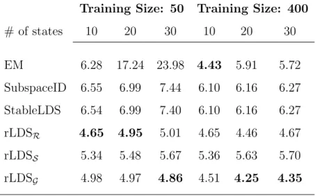
4 Average-MAPE results on the clinical data with different training sizes. . . . 47
5 Average-MAPE results on flourprice dataset. . . 59
6 Average-MAPE results on evap dataset. . . 59
7 Average-MAPE results on h2o evap dataset. . . 59
8 Average-MAPE results on clinical dataset. . . 60
9 Ten lab tests from the CBC panel. . . 70
10 Clinical acceptance categories. . . 74
11 MAE on CBC test samples for overall prediction tasks. . . 114
12 MAE on CBC test samples for short-term prediction tasks. . . 116
13 Clinical evaluation for overall prediction. . . 120
14 Clinical evaluation for short-term prediction. . . 120
15 Average-MAPE results (means and standard errors) for the different initial observation sequence lengths. reGP and reMTGP are short for rLDS+reGP and rLDS+reMTGP. The best performing method is shown in bold. Also in bold are the methods that are not statistically significantly different from the best method at 0.05 significance level. . . 121
16 Average-MAPE results (means and standard errors) of all models in the pool and two wFTL methods for the different initial observation sequence lengths. The best performing method is shown in bold. Also in bold are the methods that are not statistically significantly different from the best method at 0.05 significance level.. . . 123 17 Average-MAPE results (means and standard errors) of the proposed wFTL
approaches compared to the ensemble and online methods for the different initial observation sequence lengths. The best performing method is shown in bold. Also in bold are the methods that are not statistically significantly different from the best method at 0.05 significance level. . . 125 18 Average-MAPE results (means and standard errors) of the proposed wFTL
approaches compared to the subpopulation methods for the different initial observation sequence lengths. The best performing method is shown in bold. Also in bold are the methods that are not statistically significantly different from the best method at 0.05 significance level. . . 127 19 Average-MAPE results (means and standard errors) of the proposed wFTL
approaches compared to the model adaptation based methods for the different initial observation sequence lengths. reGP and reMTGP are the abbreviations for rLDS+reGP and rLDS+reMTGP. The best performing method is shown in bold. Also in bold are the methods that are not statistically significantly different from the best method at 0.05 significance level. . . 128
LIST OF FIGURES
1 A regularly sampled ECG time series fragment. . . 5
2 An irregularly sampled MCHC lab test time series. . . 6
3 The four categories of clinical time series forecasting problems. . . 8
4 The graphical representation of the LDS. . . 14
5 Irregularly sampled time series discretization by using DVI. . . 18
6 Irregularly sampled time series discretization by using WbS. . . 19
7 The graphical illustration of WbS with overlaps. . . 20
8 The graphical illustration of GP prior and posterior. . . 22
9 The prediction problem on a GP model on irregularly sampled time series data. 23 10 The graphical illustration of our rLDS model. . . 35
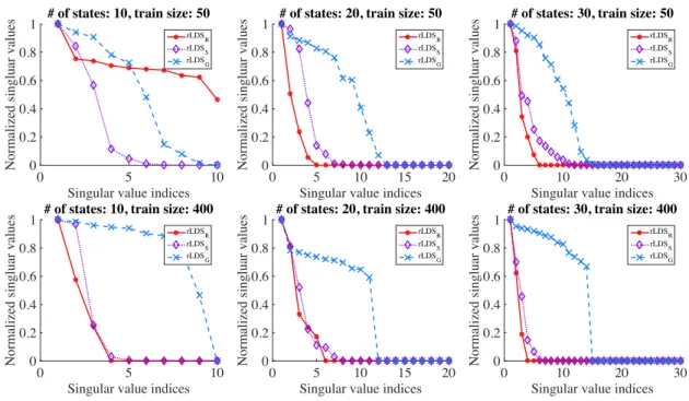
11 State space recovery on a synthetic dataset. . . 44
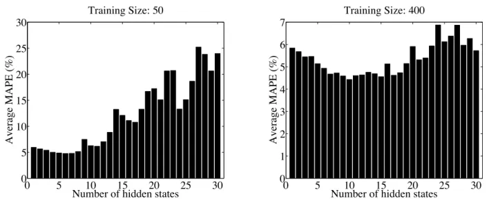
12 LDS overfitting phenomena.. . . 45
13 State space recovery on the clinical data. . . 46
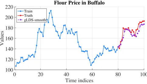
14 Predictions for flour price series in Buffalo by using gLDS-smooth. . . 58
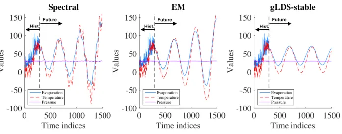
15 Simulated sequences from gLDS-stable model in evap data. . . 60
16 Intrinsic dimensionality recovery in flourprice data.. . . 61
17 The graphical illustration of the hierarchical dynamical model. . . 65
18 Time series for ten tests from the CBC panel for one of the patients. . . 71
19 MAE on MCV and RBC test samples for random prediction tasks. . . 73
20 Clinical evaluations of HDSGL on MCV and RBC. . . 74
22 Average-MAPE results of all models in the pool and two wFTL methods for
the different initial observation lengths. . . 92
23 Average-MAPE results of the proposed wFTL approaches compared to the ensemble and online methods. . . 94
24 Average-MAPE results of the proposed wFTL approaches compared to the subpopulation methods. . . 95
25 Average-MAPE results of the proposed wFTL approaches compared to the model adaptation based methods. . . 96
26 Predictions for flour price series in Minneapolis by using gLDS-smooth. . . . 109
27 Predictions for flour price series in Kansas City by using gLDS-smooth. . . . 110
28 Simulated sequences from gLDS-stable model in fourprice data. . . 111
29 Simulated sequences from gLDS-stable model in h2o evap data. . . 112
30 Simulated sequences from gLDS-stable model in clinical data for one patient. 112 31 Intrinsic dimensionality recovery in evap data. . . 113
32 MAE on ten CBC lab tests for overall predictions. . . 115
33 MAE on ten CBC lab tests for short-term predictions. . . 117
LIST OF ALGORITHMS
1 Proximal descent algorithm for solving eq.(3.3). . . 38
2 Incremental proximal descent algorithm for solving eq.(3.9). . . 40
3 Parameter estimation in rLDS . . . 41
4 Learn the LDS model in gLDS. . . 51
5 Learning and Prediction Procedures . . . 81
6 Kalman filter algorithm for LDS . . . 103
PREFACE
I spent six fabulous years in Pittsburgh. I would like to thank the people who accompanied me and made my journey of pursing Ph.D. possible and pleasurable.
First of all, I want to sincerely thank my research advisor Dr. Milos Hauskrecht. This dissertation would be impossible to complete without the help from Milos. He not only taught me the advanced machine learning and data mining techniques but guided me through the scientific research process. His high professional standards and rigorous attentions to details helped me solve real-world clinical problems, publish top conference and journal papers, obtain the Andrew Mellon Predoctoral Fellowship for the school year 2015-2016 and gradually shape my logical thinking and problem solving skills. Thank you, Milos!
I would also like to thank my Ph.D. committee members, Dr. Rebecca Hwa, Dr. Jingtao Wang and Dr. Christos Faloutsos for their valuable suggestions and insightful discussions during my proposal and dissertation defenses. I want to thank our post-doc Lei Wu, with whom I worked during my first year of Ph.D. research and also other members of Milos’ machine learning group: Shuguang Wang, Quang Nguyen, Dave Krebs, Eric Heim, Charmgil Hong, Salim Malakouti, Siqi Liu and Zhipeng Luo.
I was privileged to work as an intern in Google Inc., eBay Research Lab, Yahoo! Labs and Alibaba Group with amazing colleagues and mentors: Laura Werner from Google Inc; Nish Parikh, Gyanit Singh, and Neel Sundaresan from eBay Research Lab; Chris Yan Yan, Jimmy Jian Yang, Pengyuan Wang, Wei Sun, James Li, and Zheng Wen from Yahoo! Labs; Jian Xue, Shenghuo Zhu, Sen Yang, Jian Tan and Rong Jin from Alibaba Group. The internship experience taught me both the research & development paradigm in the industry. I learned how to quickly adapt in new environments and how to openly communicate with others.
I am very grateful to have so many wonderful friends throughout my educational odyssey. I need to mention Xiangmin Fan, Rui Wu, Lingjia Deng, Jiannan Ouyang, Ka Wai Yung, Wencan Luo, Lanfei Shi, Mengmeng Li, Huichao Xue, Wenting Xiong, Yingze Wang, Yao Sun and Yu Du for marvelous times we spent together in Pittsburgh. I made great friends at both Pitt and CMU, with whom I would like to keep in touch including Lailuyun Xu,
Rongqian Ma, Shou Li, Shicheng Lv, Yangzhan Yang, Haifeng Xu, Xuelian Long, Bo Luan, Yingjun Su, Yun Wang, Rui Liu, Guimin Lin, Guangyu Xia, Xi Chen and others.
I would also like to thank colleagues and friends who I met during academic conferences and internships. We often exchanged research ideas interdisciplinarily, which broadened my sight and encouraged me to move forward. In particular, I would like to thank Huan Liu, Jieping Ye, Hanghang Tong, Fei Wang, Jiliang Tang, Xia Hu, Bing Hu, Chen-Yu Lee, Zixuan Wang and Shumo Chu.
Lastly, it is most important to thank my parents Tiejun and Lihua, whose unlimited patience, love, encouragement and support helped assure that I would complete this most difficult journey.
1.0 INTRODUCTION
1.1 MOTIVATION
Recent advances in data collection, data storage and information technologies have resulted in enormous collections of time series data in various aspects of our everyday life, such as sequences of weather temperature measurements reflecting the changes of the climate, clinical observations showing the health conditions of patients, or stock price series indicating the dependences and variations of the capital market. The emergence and availability of time series data provide us with a unique opportunity to gain novel insights into the processes generating the data and let us build models we can utilize for making future decisions. For example, understanding how the supply and demand change over time provides better strategies for supply chain and inventory management and planning [Aburto and Weber, 2007]. Time series analysis is the field of research that attempts to analyze these rich time series data in order to extract their meaningful statistics and infer their future behaviors.
As one important type of time series data, clinical multivariate time series (MTS) record the values of many clinical variables over time. In general these variables include various laboratory tests, physiological measurements, or treatments and are highly related to patient condition and outcomes. With the recent development of advanced data technology, large temporal electronic health record repositories emerge and become highly available. They reflect different responses and behaviors of individual patients whether this is in context of chronic or acute clinical condition, or their combination. Clinical time series data provides us with a unique opportunity to gain novel insights into the dynamics of the patient state, dynamics of the disease, or efficacy of its treatments.
1.2 TIME SERIES RELATED TASKS
With the emergence and availability of the huge amount of time series data, various of time series analysis tasks are researched and studied largely in any domain of applied science and engineering, which involves temporal measurements, such as econometrics [Zellner and Palm, 1974], signal processing [Cohen, 1995], mathematical finance [Taylor, 2007]. In the following, we briefly list several major types of time series analysis tasks which are appropriate for different purposes.
• Time series classification. Time series classification is to build a classification model based on labeled time series and then use the model to predict the label of unlabeled time series. There are many practical applications of time series classification, such as classifying electroencephalography signals [Xu et al., 2004], personal motion trajectories [Shotton et al., 2013], speech recognition [Rabiner, 1989] and more.
• Time series segmentation. In time series segmentation, the goal is to split time series data into sequences of segments by identifying the segment boundary points, and to char-acterize the dynamical properties associated with each segment. A typical application of time series segmentation is speaker diarization, in which an audio signal is partitioned into several pieces according to who is speaking at what times [Tranter and Reynolds, 2006].
• Time series outlier detection. Time series outlier detection is similar to event de-tection but focuses on finding the observation that appears to deviate markedly from other observations in the time series. Outliers may occur due to various reasons, such as machine malfunctioning, networking disturbances, or human inappropriate operations. A practical application scenario of time series outlier detection is that in clinical deci-sion support systems, temporal outlier detection algorithms can identify unusual clinical management patterns in individual patients and raise alarms if wrong treatments are detected [Hauskrecht et al., 2013].
• Temporal pattern abstraction. Temporal pattern abstractions aim to convert time series variables into time-interval sequences of abstract states or temporal logic to rep-resent temporal interactions among multiple states and define and construct temporal
patterns from these abstract representations. Temporal patterns provide appealing ab-stractions of the original time series and improve the performance for other time series tasks like time series classification [Batal et al., 2011], event detection [Batal et al., 2012].
• Temporal dependence/causal discovery. Uncovering the temporal dependent or causal relationship among MTS data is a major task in data mining, which easily finds applications in many domains. For example, in the climatology, the causal relationships between climate time series variables help identify the factors that impact the climate patterns of certain regions. In social networks, the temporal dependence improves the pattern identification of influence among users and how topics activate or suppress each other [Bahadori and Liu, 2013,Cheng et al., 2014].
• Time series forecasting. Time series forecasting is the use of a model to predict future values based on previously observed values, which has extensive applications in many do-mains. For example, in the clinical domain, accurate predicting the patients’ lab tests values from previous measurements observed by physicians will help detect an adverse event or a disease in its early stages, thus allowing clinicians to identify the most effective treatment [Osorio et al., 1998,Richman and Moorman, 2000,Liu and Hauskrecht, 2015a]. In this dissertation, we mainly focus on the task of time series forecasting, especially the forecasting problems in clinical domain. With a wide adoption and availability of elec-tronic health records (EHRs), the development of forecasting models of clinical MTS and tools for their analysis is becoming increasingly important for meaningful applications of EHRs in computer-based patient monitoring, adverse event detection, and improved patient management [Bellazzi et al., 2000,Clifton et al., 2013,Lasko et al., 2013,Liu and Hauskrecht, 2013,Liu et al., 2013,Schulam et al., 2015,Ghassemi et al., 2015,Durichen et al., 2015].
1.3 CHALLENGES
A large spectrum of temporal models have been developed and successfully applied in time series analysis [Du Preez and Witt, 2003,Ljung and Glad, 1994] and many of them have
been applied recently to support predictions or inferences on clinical and biomedical data. Example applications include detection and early warning of patient deteriorations [Clifton et al., 2013], discovery of phenotypes and endotypes [Lasko et al., 2013,Schulam et al., 2015], assessment of severity of patient’s illness [Ghassemi et al., 2015], models for active motion compensation to precisely radiate tumors in the liver or lung [Durichen et al., 2015]. How-ever, none of the aforementioned methods can be directly applied into forecasting problems in real-world clinical MTS data. Building forecasting models from EHRs encounters numer-ous challenges due to three practical characteristics of real-world clinical time series data:
multivariate behaviors, irregular samples and patient variability, which make conventional methods inadequate to handle them.
1.3.1 Multivariate Behaviors
A univariate time series is a sequence of measurements of the same variable collected over time while a multivariate time series (MTS) consists of sequences of measurements of multi-plevariables over time and exhibits complex temporal behaviors. MTS data appear in a wide variety of fields, such as health care [Sacchi et al., 2007,Hauskrecht et al., 2010a,Ho et al., 2003], economics [Kling and Bessler, 1985], motion capture [Li et al., 2009], astronomy [ Scar-gle, 1982], weather forecasting [Gneiting and Raftery, 2005], earthquake prediction [Scholz et al., 1973] and many more. MTS not only show the temporal dependent behaviors within each time series but exhibit interactions and co-movements among different time series. For example, in economics, forecasting consumer price index usually depends on money supply, index of industrial production and treasury bill rates collectively [Kling and Bessler, 1985]. In clinical domain, a large number of clinical variables might be measured for a single patient (e.g., white blood cell counts, creatinine values, cholesterol levels, etc.) [Batal et al., 2012].
A large number of hidden variable models are proposed in past decades to model such complex dependent MTS, such as hidden Markov models (HMM) [MacDonald and Zuc-chini, 1997], factorial HMM [Ghahramani and Jordan, 1997], hierarchical Bayesian mod-els [Berliner, 1996], Markov switching models [McCulloch and Tsay, 1994,Kim, 1994]. Hid-den variables empower the models to capture more variabilities in the MTS and let human
knowledge easily be incorporated in the modeling process. However, since the observational sequences in MTS data may exhibit strong interactions and co-movements, given the MTS sequences, it is difficult to seek the intrinsic dimensionality of the hidden variables. Open questions arise such as how many hidden variables are needed to sufficiently represent the MTS well?, what is the compact representations of the observation sequences? Furthermore, after introducing the hidden variables, it becomes challenging to incorporate constraints in the model learning process to achieve desired properties, such as smoothness, stability, etc. Questions emerge such as Can we easily guide the learning process by adding constraints?
1.3.2 Irregular Samples
We say that the time series is regularly sampled if the time elapsed between consecutive observations is uniform (the same for all pairs of consecutive observations), while the irregu-larly sampled time series means sequential observations are collected at different times, and the time elapsed between two consecutive observations may vary [Adorf, 1995].
Usually we obtain regularly sampled time series through sensor devices which regularly collect observations at some fixed sampling frequency. For example, due to the advances of health care sensor technologies, we can easily record the regularly sampled electrocardiogram (ECG) and electroencephalogram (EEG) signals (depicted in Figure 1). In the climatology, weather stations set climate sensors to collect the outside temperature, wind speed, humidity at regularly sampled time stamps.
Time indices 275 276 277 278 279 280 281 282 283 Normalized values -4 -2 0
2 A regularly sampled ECG time series
However, in many situations we observe irregularly sampled time series, which is very dif-ferent from typical regularly sampled time series domains. For example, in clinical domain, the observations are obtained whenever a patient visits a healthcare facility and the time intervals between consecutive visits tend to vary greatly. Even during a patient’s hospital-ization, there is no guarantee that the physician can order lab tests regularly. An irregularly sampled mean corpuscular hemoglobin concentration (MCHC) lab test time series from a patient is shown in Figure 2.
Time indices 0 200 400 600 800 1000 Normalized values -1 -0.5 0 0.5
1 An irregularly sampled MCHC time series from a patient
Figure 2: An irregularly sampled MCHC lab test time series.
This irregularly sampled data preclude the applications of a large class of time series modeling techniques that require regularly sampled observations. Modeling irregular sam-pled questions gives rise to numerous important questions like Can we still use existing discrete time models to model the irregularly sampled time series?,Is it possible to model the irregular sampled data directly?
1.3.3 Patient Variability
Clinical MTS exhibits large patient variability. First, the number of observations in each patient sequence is limited and the duration they span may vary a lot from patient to pa-tient. As we discussed in Section 1.3.2, nowadays we can easily obtain a long-span time series via sensor devices by either increasing the sampling frequency or keeping it recording for a longer period of time. However, compared to the long-span time series data, patients are usually hospitalized for short periods of time (often less than two weeks), which produces
relatively short-span clinical sequences (often less than 50) [Liu et al., 2013]. Second, within each patient specific clinical MTS sequence, values of various laboratory tests, physiological measurements, or treatments are all recorded. They reflect different responses and behaviors of individual patients and contain lots of short-term variability due to different causes [ Schu-lam et al., 2015]. For example, the blood tests may be affected by events like infection, bleeding, transfusion, or a particular medication treatment.
All such patient variability poses two hard modeling problems of supporting accurate predictions for each patient. First, given a complex length-varying MTS collection,how can we learn a population based forecasting model without overfitting to such short-span temporal data? Second, patient-to-patient variability is typically large and population based models derived or learned from many different patients are unable to capture short-term variability in each individual patient. Given a patient specific prediction task, how can we adapt the population based model to provide accurate personalized predictions?
1.4 CONTRIBUTIONS
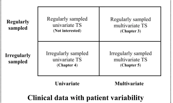
In this dissertation we focus on the time series forecasting of clinical data with large patient variability (Section1.3.3). To better understand the forecasting challenges and have a clearer overview of completed work discussed in this dissertation, we introduce four categories of forecasting problems formed by the intersection of two of the three characteristics discussed previously (depicted in Figure3). Categories are defined by whether they consider univariate or multivariate time series and whether they consider regularly or irregularly sampled data. Below we explain the corresponding problem in each category and highlight our contribution in those categories.
Forecasting regularly sampled univariate time series is the simplest case depicted in the top left in Figure 3. Observations within each time series are obtained at a fixed sampling frequency and forecasting is conducted individually. Many existing forecasting methods can be applied to such time series data, such as ARIMA [Box and Pierce, 1970,Makridakis and Hibon, 1997], exponential smoothing [Gardner, 1985], polynomial regression [Theil, 1992].
Irregularly sampled univariate TS (Chapter 4) Regularly sampled univariate TS (Not interested) Regularly sampled multivariate TS (Chapter 3) Irregularly sampled multivariate TS (Chapter 5) Irregularly sampled Univariate Regularly sampled Multivariate
Clinical data with patient variability
Figure 3: The four categories of clinical time series forecasting problems.
Furthermore, methods from other categories generally can be applied to model regularly sampled univariate time series with few or no modifications. Therefore, in this dissertation, we will focus more on forecasting problems in other categories in Figure 3.
In Chapter 3, we develop two frameworks to learn temporal models from regularly sam-pled multivariate time series data. Our work focuses on the refinements of a popular model for MTS analysis: the linear dynamical system (LDS) (described in Section 2.2.1). More specifically, the first framework, regularized linear dynamical system, aims to automatically identify the intrinsic dimensionality of the hidden state space of LDS given a limited number of MTS data and consequently, prevents the overfitting problem and performs more accurate forecasting. We develop a maximum a posteriori learning framework to learn the regular-ized LDS models from a small amount of complex MTS data. In our learning framework, we choose parameter priors to bias the model towards a low-rank solution. We propose three strategies for choosing the parameter priors that lead to three instances of our regu-larized LDS. The second framework is developed for learning LDS models from a collection
of MTS data based on matrix factorization, which is different from traditional EM learning and spectral learning algorithms. In our generalized LDS learning framework, each MTS sequence is factorized as a product of a shared emission matrix and a sequence-specific (hid-den) state dynamics, where an individual hidden state sequence is represented with the help of a shared transition matrix. One advantage of our generalized framework is that various types of constraints can be easily incorporated into the learning process. Furthermore, we propose a novel temporal smoothing regularization approach for learning the LDS model, which stabilizes the model, its learning algorithm and predictions it makes. We demonstrate the benefits of our methods on a number of time series data sets.
In Chapter 4, we focus on challenges in forecasting from irregularly sampled data. Since observations that form clinical time series are usually are made initiated (ordered) by a clinician, no fixed sampling frequency can be guaranteed. In this chapter, we propose and develop a novel hierarchical dynamical system framework for modeling clinical time series that combines advantages of the two temporal modeling approaches: the linear dynamical system and the Gaussian process(GP). We model the irregularly sampled clinical time series by using multiple GP sequences in the lower level of our hierarchical framework and capture the transitions between GPs by utilizing the LDS. The experiments are conducted on the complete blood count (CBC) panel data of 1000 post-surgical cardiac patients during their hospitalization. We show that our model outperforms multiple existing models in terms of the mean absolute prediction error and the absolute percentage error. Our method achieved a 3.13% average prediction accuracy improvement on ten CBC lab time series when it was compared against the best performing baseline. A 5.25% average accuracy improvement was observed when only short-term predictions were considered.
In Chapter 5, we develop and study personalization strategies for building improved forecasting models that better mimic patient specific behaviors from irregularly sampled multivariate clinical data. This problem is rather challenging due to the characteristics of clinical MTS and the computational and modeling trade-offs arising from them. Briefly, when the time series of past observations for the patient are short, it may be hard to learn a patient specific model, and the population based model may be a better option. On the other hand, when the observed data for the target patient are sufficiently long, a patient
specific time series model may better reflect the future behavior. In this dissertation, we develop two approaches to address the above issues. Our first approach builds upon model adaptation. It first learns a population based model from all the available patients and then re-calibrates the population based model into personalized models through patient specific residual models. The patient specific residual models are learned from multivariate residual time series, which is the difference between the patient observations and the population based model’s predictions. The second approach relies on adaptive model selection strategies to combine advantages of the population based, patient specific and short-term individualized predictive models. We build a pool of high quality forecasting models for clinical MTS and their variety assures the coverage of many different modes and behaviors. Our approach is designed to pick the most appropriate predictive model for each patient at every time stamp. Both proposed approaches are evaluated on a real-world clinical time series data set. The results demonstrate that our approaches are superior on the prediction tasks for irregularly sampled multivariate clinical time series, and they outperform pure population based and patient specific models, as well as, other patient specific model adaptation strategies in terms of prediction accuracy.
1.5 OUTLINE
The rest of this dissertation is organized as follows: Chapter 2 introduces the notation to be used in subsequent chapters and provides a review of the basics of time series models and the personalized predictive methods to guide the precision medicine. Chapters3,4 and 5 present the main contributions of this dissertation. Finally, Chapter 6 summarizes the contributions of this dissertation and discusses avenues of future work.
Finally, I would like to note that parts of this dissertation have been previously published in the following conferences and journal: SDM 2013 [Liu et al., 2013], AIME 2013 [Liu and Hauskrecht, 2013], AAAI 2015 [Liu and Hauskrecht, 2015b], AAAI 2016 [Liu and Hauskrecht, 2016a], SDM 2016 [Liu and Hauskrecht, 2016b] and the Artificial Intelligence in Medicine [Liu and Hauskrecht, 2015a].
2.0 BACKGROUND
In this section, we first define notation used in this dissertation. Then, we review the basics of the time series models, in particular, (1) the linear dynamical system, which is a discrete time model used commonly to represent regularly sampled time series data (Section2.2.1); (2) the Gaussian process model that works with continuous real-valued quantities and lets us model functions of continuous time (Section 2.2.2); and (3) the multi-task Gaussian process model that extends the standard Gaussian process to model the multivariate dependence within multivariate time series (Section 2.2.3). After that, we review various techniques used in biomedical and clinical domains to build predictive patient specific models. These techniques are proposed to entail the delivery of individually tailored clinical decision supports that leverage information about each person’s unique characteristics, which can be summarized into three categories: subpopulation models (Section2.3.1), model adaptation (Section2.3.2) and adaptive model selection (Section 2.3.3).
2.1 NOTATION
In the following, we introduce the notation that be used in the subsequent.
• We denote time series data D as a collection of N multivariate time series sequences
D = {Y1,Y2,· · · ,YN}. Each Yl consists of a sequence of T
l past observation-time
pairs (yil, tli), i.e., Yl ={(yli, tli)Tl
i=1}, such that Tl is the number of past observations for
sequence l, 0< ti < ti+1, andyil is an-dimensional observation vector made at time (ti). n is the number of clinical variables in the MTS.
• Let N(m,Σ) be a multivariate normal distribution with the mean vector mand covari-ance matrix Σ. Let Ez[f(·)] denote the expected value of f(·) with respect to z.
• Special norms used throughout this work include: k · kF, k · k∗, k · k2 and k · k1 which
is the matrix Frobenius norm, the matrix nuclear norm, the vector Euclidean norm and the vector/matrix `1 norm.
• For both vectors and matrices, the superscript > denotes the transpose. vec(·) denotes the vector form of a matrix; and ⊗ represents the Kronecker product. Tr is the trace
operator and Id is the d×d identity matrix.
For the sake of notational brevity, we omit the explicit sample index (“l”) and describe our methods by using a MTS sample for the rest of this section. However, it is worth to note that methods we developed can be applied to data of multiple time series samples with few or no modifications.
2.2 TIME SERIES MODELS
A large spectrum of models have been developed and successfully applied in time series mod-eling and forecasting [Hamilton, 1994], such as ARIMA [Box and Pierce, 1970,Makridakis and Hibon, 1997], exponential smoothing [Gardner, 1985], etc. However, the majority of existing models are focused on regularly sampled univariate time series. In the following, we first review the basics of the linear dynamical system, which is used commonly to represent multivariate time series data (Section 2.2.1). Then, we review the basics of the Gaussian process model that works with continuous real-valued quantities and lets us model functions of continuous time (Section 2.2.2). After that, we introduce the multi-task Gaussian process model, which is an extension of Gaussian process model for multivariate time series (Section 2.2.3).
2.2.1 Linear Dynamical System
The linear dynamical system (LDS) is a classical and widely used model for real-valued sequence analysis [Kalman, 1963], that is applicable to many real-world domains, such as engineering, astronautics, bioinformatics, economics [Lunze, 1994,Liu and Hauskrecht, 2013]. This is due to its relative simplicity, mathematically predictable behavior, and the fact that exact inference and predictions for the model can be done efficiently [Martens, 2010].
The LDS is an MTS model that represents observation sequences indirectly with the help of hidden states. Similarly yi and Y we introduced in Section 2.1, let zi be a d×1 vector
representing the values of d dimensional hidden states at time stamp ti corresponding to yi
and denote Z as a d×T matrix representing the entire values of hidden states along the time span T. The LDS model is a discrete time model which assumes all the time stamps within a sequence are evenly spaced, i.e.,ti+1−ti = Φ and Φ is the constant representing the
fixed length of time interval. The LDS models the dynamics of these sequences in terms of the state transition probability p(zi|zi−1), and state-observation probability p(yi|zi). These
probabilities are modeled using the following equations:
zi =Azi−1+i (2.1)
yi =Czi+ζi (2.2)
where the transitions among the current and previous hidden states are linear and captured in terms of a d×d transition matrix A. The stochastic component of the transition, i, is
modeled by a zero-mean Gaussian noise i ∼ N(0, Q) with a d×1 zero mean vector and
a d×d covariance matrix Q. The observations sequence is derived from the hidden states sequence. The dependencies in between the two are linear and modeled using an n× d
emission matrixC. A zero mean Gaussian noiseζi ∼ N(0, R) models the stochastic relation in between the states and observations. In addition toA, C, Q, R, the LDS is defined by the initial state distribution forz1 with meanξand covariance matrix Ψ, i.e.,z1 ∼ N(ξ,Ψ). The
complete set of the LDS parameters is Λ ={A, C, Q, R,ξ,Ψ}. The graphical representation of the LDS is shown in Figure 4.
yi
yi 1
z
i 1z
iN
Figure 4: The graphical representation of the LDS. Shaded nodes yt and yt−1 denote
ob-servation made at current and previous time steps. Unshaded nodes zt and zt−1 denote the
corresponding hidden states. The links represent dependences among the observations and hidden states. The plate represents a collection of N sequences.
2.2.1.1 Applications The LDS model is a powerful tool in the analysis of the evolution of a dynamical model in time and is commonly used time series model for real-world en-gineering and financial applications [Isard and Blake, 1998,Kazemi et al., 2008,Victor and Alberto, 2011,Rogers et al., 2013]. In the following, we describe two important applications of the LDS models, Visual Tracking and Biomedical Signal Processing.
Visual Tracking The LDS models show numerous successful applications in visual tracking (a.k.a, object tracking), which is the problem of estimating the positions (coordi-nates) and other relevant information of moving objects from a collection of noisy observa-tions [Lee et al., 1995,Isard and Blake, 1998,Funk, 2003,Li et al., 2004,Weng et al., 2006]. In visual tracking, the LDS is robust to the noise caused by rotation, illumination changes, occlusions, etc. and the time update step and measure update step in the Kalman filtering
algorithm (see AppendixA) is able to filter out the noise from the signal measurements while retain the true trajectories (state sequences).
Biomedical Signal Processing The LDS models are widely used in tasks of analyzing biomedical signals, such as electroencephalogram (EEG), electrocardiogram (ECG) [ Geor-giadis et al., 2005,Georgiadis et al., 2007,Khan and Dutt, 2007,Kazemi et al., 2008,Sayadi and Shamsollahi, 2008]. Examples like Kazemi et al. [Kazemi et al., 2008] utilize Kalman filtering algorithm to remove the periodic noises (such as electricity grid induced noises)
from ECG signals. Georgiadis et al. [Georgiadis et al., 2005,Georgiadis et al., 2007] propose a Kalman filter based approach to dynamically estimate the event related potentials, which are the voltage changes of brain electric activity due to stimulation. Sayadi et al. [Sayadi and Shamsollahi, 2008] build a modified extended Kalman filter structure to conduct the ECG signals denoising and compression. Khan et al. [Khan and Dutt, 2007] use the hidden state estimates of LDS models to detect event-related desynchronization and synchroniza-tion, which are used to describe the decrease and increase in activity in an EEG signal.
2.2.1.2 Learning Linear Dynamical Systems While in some LDS applications the model parameters are known a priori, in the majority of real-world applications the model pa-rameters are unknown, and we need to learn them from MTS data. This can be done using standard LDS learning approaches such as the Expectation-Maximization (EM) [ Ghahra-mani and Hinton, 1996] or spectral learning algorithms [Katayama, 2005,Van Overschee and De Moor, 1996,Doretto et al., 2003].
Expectation-Maximization The EM algorithm is an iterative procedure for finding model parameters that maximizes the likelihood of observations in the presence of hidden variables. In practice, instead of maximizing the data likelihood directly, EM algorithm usually maximizes a Q function, which is the expectation of the joint probability of both observed and hidden variables with respect to the distribution of hidden variables. The Q function is a lower bound of the true data likelihood and maximizing it will improve the data likelihood. Under the setting of learning standard LDS defined by eq.(2.1) and eq.(2.2), the
Qfunction is defined as follows:
Q=EZ h logp(Z,Y)i =EZ h logp(z1) i +EZ hXT i=1 logp(yi|zi) i +EZ hXT i=2 logp(zi|zi−1) i (2.3)
The EM algorithm alternates between maximizing the Q function with respect to the parameters Λ and with respect to the distribution of hidden states, holding the other quan-tity fixed. The E-step depends on E[zi|Y], E[ziz>i |Y] and E[ziz>i−1|Y], which are sufficient
statistics to compute eq.(2.3). Detailed algorithms for computing the sufficient statistics are provided in Appendices A and B. The M-step re-estimate each of the parameter in Λ by
taking the corresponding partial derivative of the expected log likelihood, setting to zero and solving.
Spectral Learning Spectral learning methods provide a non-iterative, asymptotically unbiased LDS estimation solution in closed form. They estimate the parameters of an LDS by using singular value decomposition (SVD) to find Kalman filter estimates of the underlying state sequence [Katayama, 2005,Van Overschee and De Moor, 1996,Doretto et al., 2003]. Spectral learning methods approximate the observation matrixYor its variants (hankel matrix) [Boots et al., 2007] into UΣV0 by SVD, where U ∈ Rn×d and V ∈ RT×d
have orthonormal columns {ui} and {vi} and Σ = diag{δ1,· · · , δd} contains the singular
values. The emission matrix and state sequence are estimated as ˆC = U and ˆZ = ΣV0
and the transition matrix is obtained by solving the least square of kAZ1:T−1 −Z2:Tk2F
where Za:b represents a subsequence of Z inclusively from the time ta to timetb, i.e., Za:b =
[za,za+1,· · · ,zb−1,zb].
Due to iterative re-estimation the EM is slower than spectral methods that do not iter-ate. However, the maximum likelihood solution found by EM might provide more accurate parameter estimation than spectral learning methods, especially when the amount of train-ing data is small, but is subject to local optima. In practice, the estimates from spectral learning are used as the initialization of the EM algorithm [Boots et al., 2007].
However, even though the standard EM and spectral methods are maturely developed, learning LDS from short-span low-sample clinical MTS data set encounters a number of questions. First, both EM and spectral methods require to know the intrinsic dimensionality of an LDS’s hidden state space in advance, which in general is difficult. The dimensionality plays an important role in the performance of LDS models due to the fact that a small number of hidden states may not be able to model the complexities of a MTS, while a large number of hidden states can lead to overfitting. In Section 3.1 of this dissertation, we address the above issue by presenting a regularized LDS framework to recover the intrinsic dimensionality of MTS and consequently prevent model overfitting given short MTS data sets. Second, neither the EM algorithm nor spectral methods are able to constrain the LDS learning process in the sense of leading the learned models to achieve desired properties, such as stability. In Section 3.2 of this dissertation, we propose and develop a generalized
LDS learning framework in which various constraints are easily incorporated and parameter optimizations are efficiently conducted.
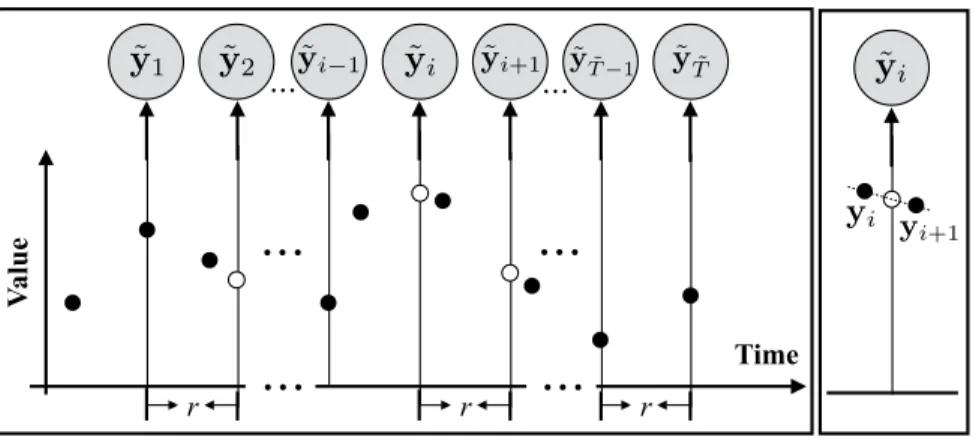
2.2.1.3 Irregularly Sampled Data Discretization In general, there are two ways to handle irregularly sampled time series data and convert them to observation sequences one can model and analyze using the discrete time models: (1) direct value interpolation (DVI) approach and (2) window-based segmentation (WbS) approach. In the following we briefly summarize these two approaches.
Direct Value Interpolation The DVI approach assumes that all observations are col-lected regularly with a pre-specified sampling frequencyr. However, instead of actual read-ings the values at these time points are estimated from readread-ings at time points closest to them using various interpolation techniques [Adorf, 1995,Dezhbakhsh and Levy, 1994,˚Astr¨om, 1969]. The interpolated (regular) time series, i.e., ˜Y ={(˜yi,t˜i)
˜ T
i=1}, is then used to train a
discrete time model such as LDS. The approach is illustrated in Figure5. We put a tilde sign (˜·) over Y and yi to indicate the discretized observations. ˜ti is time stamps of discretized
observations and ˜T is the length of discretized sequence. In terms of predictions of future values, one has to first use trained discrete time model to predict the values at time points closest to the target time, and after that, apply the interpolation approach to estimate the target value.
The DVI approach converts the time series with irregular observations to discrete time observation sequences. The quality of the conversion depends on the number of observations actually seen and the sampling frequency parameter r. One straightforward way to set r
is to use internal cross-validation approach. Briefly, we divide the time series data used for training the models into folds and use them to built multiple internal training and testing datasets. The models built with different sampling frequencies r are tested on the internal test sets, and the best r that leads to the best prediction accuracy on the internal test data (averaged over different folds) is selected.
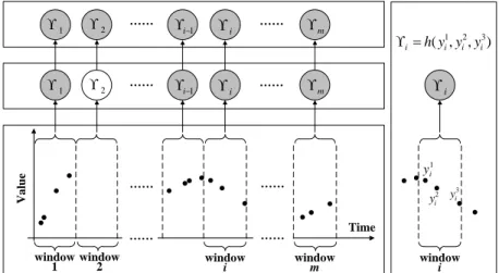
Window-based Segmentation The WbS approach is slightly different. Instead of values at pre-specified regularly sampled time points, the approach first segments time series to fixed-sized windows. The behavior in the window is summarized in terms of its statistics
r r r Time V al u e ˜ y1 y˜2 y˜i 1 y˜i y˜i+1 y˜T˜ 1 y˜T˜ yi yi+1 ˜ yi
Figure 5: Transformation of an irregularly sampled time seriesY ={(yi, ti)Ti=1}to a discrete
time series ˜Y ={(˜yi,˜ti) ˜ T
i=1} by using DVI. The empty circles denote the interpolated values
with no readings. The right panel illustrates the linear interpolation process.
γ, such as, the mean, or the last value observed within that time interval [Chu, 1995,Das et al., 1998,Yi and Faloutsos, 2000,Keogh and Pazzani, 2000,Keogh et al., 2001,Smyth and Keogh, 1997]. The values generated by the different windows define sequences of γ
statistics. The discrete time model is then used to represent how the summary statistics
γ in two consecutive windows change, that is, a sequence of statistics calculated over these intervals are considered to be observations of the discrete time model. Predictions at future times for the window-based approach are made using the discrete time model by identifying the time interval the target time point falls into.
We would like to note that in order to learn the parameters of the window-based discrete time model from irregularly sampled data one has to either assure that every time interval has at least one reading that is sufficient to calculate the summary statistics; or impute the statistics for the window with missing values from its neighbors using, for example, interpolation methods. Figure 6 illustrates the process of filling statistics in intervals with missing values by using interpolations. Briefly, after segmentation of time series to windows of a fixed size (step 1), the summary statistics γi for each window i are calculated (step 2),
and for windows with no readings, the statistics are interpolated from windows next to it (step 3). Once the missing statistics are imputed, the discrete time models, such as LDS,
can be learned from complete sequences γ1, γ2,· · ·, γm of summary statistics derived from
time series data.
Time V a lu e window
1 window2 windowi windowm
…… …… 1 2 i1 i m …… …… …… …… …… …… Step 1 Step 2 Step 3 1 i y 2 i y yi3 1 2 3 ( , , ) i h y y yi i i 1 2 i1 i m window i i
Figure 6: Transformation of irregularly sampled time series Y = {(yi, ti)Ti=1} to a discrete
time series γ ≡ {γi}by WbS. The shaded nodes denote summary statistics calculated from
the corresponding windows, such asγi in step 2. The regular (unshaded) nodes denote empty
summary statistics corresponding to windows with no readings, such as γ2. h in the right
panel denotes the summary statistics estimation function.
The discrete time models (once they are learned) can be used for prediction by taking an initial sequence of observations for a new instance and predicting values at an arbitrary future timet∗. This is accomplished by first applying the WbS to observed data for the new instance and by calculating or imputing the statisticsγ for each window. The value at some future timet∗ is predicted by using the time series model (like LDS) to predict the statistics
γ∗ for the window the future time falls into and after that infer the value for target time t∗
fromγ∗. We note the simplest implementation of step 3 is to predict the value directly with the summary statistic. Briefly, if the summary statistic reflects the value of observations in the respective time window, we may directly use this value to predict the value for any time that falls within the corresponding window.
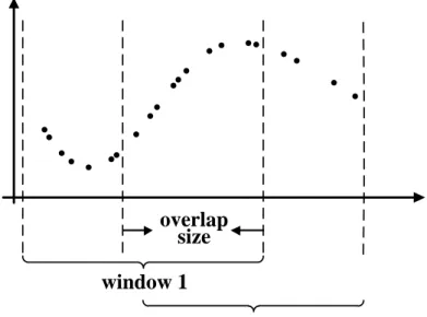
The above window-based approach can be further refined by overlapping two consecutive windows that generate the statistic γ in time. This means some of the observations can be
shared by two windows and may influence the statistics in two consecutive steps. Overlapping the two windows helps to smooth the transitions in statistics. In addition, it helps to generate longer sequences one can use to train better models. The idea of window overlap is illustrated in Figure 7. Considering windows and their overlaps, the segmentation of the time series is induced by two parameters: the window sizeW and the overlap sizeO. These are additional parameters of the WbS approach, and if needed, they can be optimized using the internal cross-validation approach.
Time
V
a
lu
e
window 1
window 2
overlap
size
Figure 7: The graphical illustration of WbS with overlaps on the irregularly sampled time series data.
2.2.2 Gaussian Process
The Gaussian process (GP) is a popular nonparametric nonlinear Bayesian model in sta-tistical machine learning [Rasmussen and Williams, 2006]. A GP is a collection of random variables, any finite number of which have a joint Gaussian distribution. The GP is best viewed as an extension of the multivariate Gaussian to infinite-sized collections of real-valued variables defining the distribution over random functions. Table 1 summarizes the relation-ship between Gaussian distribution, multivariate Gaussian distribution and the GP.
Table 1: Relationship between Gaussian distribution, multivariate Gaussian distribution and Gaussian process.
Mean type (Co)variance type
Gaussian distribution Scalar Scalar
Multivariate Gaussian distribution Vector Matrix
Gaussian process Function Function
A GP is represented by the mean function m(x) =E[f(x)] and the covariance function
KG(x,x0) =
E[(f(x)−m(x))(f(x0)−m(x0))], where f(x) is a real-valued process and x is
the input vector. The mean function m(x) indicates the central tendency of the process, and the covariance function controls the variation in terms of the similarity or distance of the two input vectors xand x0.
The GP can be used to calculate the distribution p(f(X∗)) of f values for an arbitrary set of inputs X∗. The distribution p(f(X∗)) is a multivariate Gaussian defined as follows.
f(X∗)∼ N(m(X∗), KG(X∗,X∗)) (2.4)
Eq.(2.4) defines the prior distribution of f(X∗). In addition, the GP can be used to calculate the posterior distribution p(f(X∗)|(X,Y)) of f values for inputsX∗, given a set of observed values Y for X, where Y = f(X) +, assuming additive independent identically distributed Gaussian noise with variance σ2, ∼ N(0, σ2). The posterior is again a multivariate Gaussian p(f(X∗)|(X,Y)) defined as follows.
f(X∗)|(X,Y)∼ N(m(X∗|(X,Y)), Cov(X∗|(X,Y))) (2.5)
m(X∗|(X,Y)) =m(X∗) +KG(X∗,X)KG(X,X) +σ2I−1(Y−m(X)) (2.6)
Cov(X∗|(X,Y)) = KG(X∗,X∗)−KG(X∗,X)KG(X,X) +σ2I−1KG(X,X∗). (2.7) Figure 8illustrates the examples of functions drawn from the GP prior and posterior in a 1-D space; Figure 8(a) shows functions drawn from the prior distribution function values at X∗. Figure 8(b) shows functions drawn from the posterior distributions given that some data points (X,Y) are observed.
−3 −2 −1 0 1 2 3 −3 −2 −1 0 1 2
(a) Three functions drawn at random from the zero-mean GP prior. −3 −2 −1 0 1 2 3 −3 −2 −1 0 1 2 3
(b) Three random functions drawn from the GP posterior given three observations.
Figure 8: The graphical illustration of GP prior and posterior. In this example, we create
X∗ as a linearly spaced vector from -3 to 3 with step size 0.01. We set the mean function
m(·) = 0 and covariance function KG(x, x0) = exp(−(x−x0)2/2).
2.2.2.1 Applications Due to the function view of GP methodology and its correspond-ing flexible nature, GP has a variety of applications in solvcorrespond-ing temporal modelcorrespond-ing problems. In the following, we describe two major applications of GP in time series domain.
GP as A Function of Time As we discuss in Section 2.2.2, GP can be viewed as an extension of the multivariate Gaussian distribution in the function space (infinite space) which can be directly applied to time series modeling problems by representing observations
as a function of time [Roberts et al., 2013,Girard et al., 2003,Brahim-Belhouari and Bermak, 2004]. As a result, there is no restriction on when the observations are made and whether they are regularly or irregularly spaced in time and it can be easily applied to make future time prediction. Given any time index t∗ we can calculate its posterior mean with eq.(2.6), and use it to predict the values at that time. Figure 9 illustrates this step.
Time
V
a
lu
e
t* ( ( *) | , ) p f tY X
Figure 9: The graphical illustration of the prediction problem on a GP model on irregularly sampled time series data. The solid line denotes the GP we learned from the data and the dotted line indicates the GP’s predictions of future values for future time t∗. The posterior distribution off(t∗) at timet∗ is shown and the empty circle is the mean of that distribution, which is the value predicted by the GP.
GP as A Non-linear Transformation Instead of using GP as a function of time, we can choose to use GP as a non-linear transformation operator and substitute GP for the linear transformations in traditional temporal models. For example, in the LDS model defined by eq.(2.1) and eq.(2.2), we can replace the transition matrixA and emission matrix
C, which are linear transformation operators, with two GPsr(·) andu(·). This leads to the following discrete-time Gaussian process dynamical system [Turner et al., 2010].
zi =r(zi−1) +i (2.8)
yi =u(zi) +ζi (2.9)
The transition function r(·) and the observation function u(·) represent stochastic tran-sitions and observations, and are represented with the help of Gaussian processes. i and
ζi are the same as in eq.(2.1) and eq.(2.2). Briefly, the LDS assumes linear dependencies among latent states and observations, while the GP based model replaces the linear depen-dencies with more general nonlinear functions r(·) and u(·). Please note that if zi states
are observed then the model collapses to an autoregressive model which is represented by a single GP. [Turner et al., 2010] introduced the GPIL algorithm for inference and learning in the above discrete-time Gaussian process dynamical system based on the EM framework. Similar ideas appear in [Wang et al., 2005,Wang et al., 2008,Deisenroth et al., 2009,Ko and Fox, 2011] for building nonlinear dynamic systems by utilizing GP.
2.2.2.2 Learning Gaussian Process Models The parameters of the GP are formed by parameters defining the mean and covariance functions. The mean function is the function of time and the covariance function measures the similarity of two function values based on corresponding input time stamps.
The prior mean function is considered as the expectation function, prior to any obser-vation. Usually, we are equally unsure whether the time series trend is up and down and this symmetry of ignorance leads to constant-offset mean functions [Roberts et al., 2013]. While in some cases, we do have a prior domain knowledge of the long-term trend of the time series, we can easily incorporate the specific function form into the Gaussian process models and the mean function’s parameters can be optimized by using gradient based approaches. In the clinical setting, where the focus of this thesis lies, we want to learn a function that fits many patients and their clinical time series. Since the patients may be encountered at different age and under different circumstances, there is no good way to align their time origins. Hence the only way to feasibly align them is to set their mean functions equal to a constant m(t) = M, which makes the mean function of a GP time invariant. To obtain
M, we can average all the observations from all the patients and use that averaged value as the constant M for the mean function. This gives us a constant mean which reflects many patients and their clinical time series.
To learn the parameters of the covariance function, we seek Θ that can maximize the marginal likelihood p(Y|X) [Rasmussen and Williams, 2006]. The log marginal likelihood
for GP is shown in eq.(2.10). logp(Y|X) = −1 2Y > KY−1Y−1 2log|KY| − T 2 log 2π (2.10)
where Y denotes all the training observations. KY = KG +σ2I is the covariance matrix
for the noisy observations Y and KG is the covariance matrix for noisy-free function values from function f, Y=f(X) +, ∼ N(0, σ). n is the number of observations.
The partial derivatives of the marginal likelihood with respect to each parameter θi in Θ
is shown in eq.(2.11). ∂ ∂θi logp(Y|X,Θ) =−1 2Tr KY−1∂KY ∂θi +1 2Y > KY−1∂KY ∂θi KY−1Y (2.11) where Θ represents the entire set of parameters in covariance function, Θ ={θi}.
Once we have the partial derivatives with respect to each parameter, any well developed gradient based methods can be directly applied to maximize p(Y|X).
In summary, the advantage of the GP model is that it lets us represent functions of time and their distributions, which has no restriction on when the observations are made and whether they are regularly or irregularly spaced in time. However, this approach also comes with limitations; the most serious one is that the mean function of the GP is a function of time and in order to make the GP independent of the time origin we need to set it to a constant value. However, this significantly limits our ability to represent changes or different modes in time series dynamics. In Chapter 4of this dissertation, we propose a new hierarchical dynamical system for modeling irregularly sample univariate time series, which combines the advantages of the LDS and GP models. A combination of the two appears as the best solution to offset their limitations.
2.2.3 Multi-task Gaussian Process
One limitation of applying GP to clinical MTS is that each clinical time series is modeled independently within a patient and the interactions between multiple clinical variables are neglected. To address this issue and capture the multivariate behaviors within the clinical MTS, the multi-task Gaussian process (MTGP) is proposed [Bonilla et al., 2007]. The MTGP
is an extension of GP to model multiple tasks (e.g., multivariate time series) simultaneously by utilizing the learned covariance between related tasks. MTGP uses KC to model the
similarities between tasks and uses KG to capture the temporal dependence with respect to
time stamps. The covariance function of MTGP is shown as follows:
KM =KC ⊗KG+D⊗IT (2.12)
where KC is a positive semi-definite matrix and KC
j,k measures the similarity between time
series j and time series k. D is an n×n diagonal matrix in whichDj,j is the noise variance δ2
j for the jth time series. ⊗ is the Kronecker product. Usually the MTGP model has the
computation limitation that it has O(n3T3) compared with n × O(T3) for standard GP models. However, this limitation is not as relevant in our application setting, given that the number of clinical observations is very limited and clinical time series are usually short span. The parameters of the GP based models are formed by parameters defining the mean and covariance functions. Typically, the covariance function makes sure the function values for two nearby times tend to have high covariance, while values from inputs that are far apart in time tend to have a low covariance. The parameters can be learned from data that consist of one or many examples of time series. The predictions of values at future times correspond to calculation of posterior distribution for these times.
The advantages of GP based models is that (1) with the reasonable choice of the co-variance function, GP based models are capable of capturing the short-term rapid changes in clinical time series [Clifton et al., 2013,Ghassemi et al., 2015]; and (2) GP based models can be applied to time series modeling problem by representing observations as a function of time. As a result, there is no restriction on when the observations are made and whether they are regularly or irregularly spaced in time.
2.3 INSTANCE-SPECIFIC MODELING
Building predictive models from available data is a fundamental task in machine learning. Typically, a single model is learned from a collection of training instances. After that, the
learned model is applied to all future instances. In this dissertation, we call such a model a
population based model, which is optimized to have good predictive performance on average on all the future instances.
In spite of the huge successful applications of population based models, recent research has demonstrated that learning specific models to particular instances can improve the per-formance [Visweswaran and Cooper, 2004,Gottrup et al., 2005,Visweswaran et al., 2015]. Different from the population based model learned from the entire training data, such spe-cific models are either trained on a particular instance or a group of spespe-cific instances or adjusted from the population based model according to the specific instance. In this disser-tation, such a model is referred to as aninstance-specific model. Recently, building and using instance-specific models have been shown great success in genetics, pharmacology, and other important aspects of healthcare such as personal preferences, nutrition, lifestyle, and disease, recapturing the importance of personalized health [Jørgensen, 2009,Swan, 2009,Schleidgen et al., 2013,Karkar et al., 2015,Wiley et al., 2016].
In general an instance-specific model can be achieved by:
• building instance-specific models for each instance. The instance-specific model is learned from a selected collection of similar examples out of the entire population. We refer these models to as Subpopulation Models (Section 2.3.1).
• adjusting the population based model to fit better the specific instance. This usually includes two steps: first learn a population based model from all available data and then calibrate the population based model according on the unique characteristics of each instance. We refer this approach to as Model Adaptation (Section 2.3.2).
• instance-dependently combining a pool of predictive models which are built either from the entire population or a subpopulation of instances. We refer this technique to as
Adaptive Model Selection (Section 2.3.3).
Please note that models from the above three categories are complementary and they can be combined in the prediction process. For example, the model adaptation techniques can be applied to both population based models and subpopulation models. Moreover, both subpopulation models and adaptive models can be candidate models in the pool of the
adaptive model selection approaches. In the following, we briefly review the three approaches to build the personalized model.
2.3.1 Subpopulation Models
The data available for model building (learning) purposes may cover a wide variety of past patients and their conditions. However, using all of them may bias the model towards the population mean. The most common way to alleviate the problem and build a patient specific model is to identify a subpopulation of patients most similar to