UW Biostatistics Working Paper Series
5-31-2005
A Linear Regression Framework for Receiver
Operating Characteristic(ROC) Curve Analysis
Zheng Zhang
Emory University, [email protected]
Margaret S. Pepe
University of Washington & Fred Hutchinson Cancer Research Center, [email protected]
Suggested Citation
Zhang, Zheng and Pepe, Margaret S., "A Linear Regression Framework for Receiver Operating Characteristic(ROC) Curve Analysis" (May 2005).UW Biostatistics Working Paper Series.Working Paper 253.
1. Introduction
In the field of medical diagnostic testing, the receiver operating characteristics(ROC) curve has long been used as a standard statistical tool to assess the accuracy of tests that yield continuous results. Previous research in the area focused mostly on estimating the ROC curve, such as the popular empirical ROC curve, a nonparametric estimation of the ROC curve and the LABROC procedure proposed by Metz et al. (1998).
Recently it has been recognized (Pepe, 1997 & 2000) that various factors can affect the test performance beyond the disease status. Those factors include different test settings and/or subject’s demographic data. One example is that for certain test whose test subjects include both men and women or both younger and older people, its performance may vary between men and women or between younger and older people. Pepe(2003, chapter 3) listed several factors that can affect test performance, such as factors associated with test subject or tester, test settings and severity of disease. It is therefore important to understand such influence to determine the optimal and suboptimal conditions or populations to perform such tests. If we find the test doesn’t perform well for certain condition or population, then we may need to modify the test or even develop a new test for those situations. On the other hand, if we find that a factor doesn’t influence test performance, we can relax the conditions under which the test is performed.
Comparing performance between several different tests is a special case of modelling covariate effects. When a new diagnostic test is developed, before it can be used in the practice, frequently we need to compare it with an existing test to evaluate whether the new test provides better discrimination between cases and controls. Under certain situations (e.g., cost and invasiveness of the test), a new test is favored as long as it is proven to be non-inferior to its closest competitor.
In this manuscript, we propose a linear regression framework to model covariate effect on the ROC curve. In section 2 we describe the regression procedures for comparing two
ROC curves. We illustrate our method using a pancreatic cancer data set in section 3. Using linear regression procedure for general covariate effects modelling are presented in section 4. We illustrate our method using an audiology data set in section 5. We give a summary and some closing remarks in section 6.
2. Comparing ROC Curves
2·1 Paired Tests versus Non-paired Tests
When comparing two diagnostic tests with respect to their performances, the study design needs to be considered. Pepe(2003) introduced the concepts of paired tests versus non-paired tests. If each individual in the population receives both tests, we call those tests paired tests. If the results are from two independent populations of subjects, we call those tests non-paired tests. Paired tests provide additional statistical challenge when we compare their performances since we need to account for the correlation between the test results derived from the same individual.
Since we routinely use the ROC curve to assess the performance of a continuous test, naturally we compare the performances of two tests by comparing their corresponding ROC curves. There are two main approaches to compare ROC curves: comparing summary measures(e.g. AUC) of the ROC curves or using regression methods to compare the ROC curves directly.
2·2 Comparing ROC curves by AUC statistics
The most popular approach to compare two ROC curves is based on the difference in their empirical AUC values. Denote two curves by ROCA and ROCB, write the null hypothesis
as
H0 :ROCA=ROCB (1)
Define
where AUCd e is defined to be the area under the emprical ROC curve.
The null hypothesis is tested by comparing ∆AUCd e/
q
var(∆AUCd e) with a standard
normal distribution, we call this test a Z-test based on empirical AUC statistics.
We need to point out that comparing AUC statistics is not equivalent to comparing the ROC curves. Two ROC curves that have cross-overs in the middle can have same AUC values, hence this approach is probably under-powered for settings when the two ROC curves cross.
2·3 Compare ROC Curves by Regression
Pepe (1997, 2000) developed the ROC-GLM procedure which is the first regression based method that can be used for ROC curves comparison. Pepe & Cai (2004) proposed another regression method based on placement value concept. The common setting for comparing ROC curves using regression is first to assume a parametric model for the ROC curves. Although the binormal model is often used, we will present the methods using the more general form as ROC(t) =g(α0+α1g−1(t)). Define indicator variable Xtest asXtest = 0 for
test A andXtest = 1 for test B and assume the ROC curves for both tests have the following
parametric form:
ROCtest(t) = g(α0+α1g−1(t) +βXtest+γXtestg−1(t)) (3)
The parameter θ= (α0, α1, β, γ)T. This model specifies that for test A, its ROC curve is
ROC(t) =g(α0+α1g−1(t)) (4)
and for test B, its ROC curve is
ROC(t) =g((α0+β) + (α1+γ)g−1(t)) (5)
The underlying assumptions for equation (4) is that there exists an unknown monotone increasing function hA, such that
and
hA(YD,A)∼N(α0/α1,1/α21).
Similarly, for test B, equation (5) assumes there exists an unknown monotone increasing function hB, such that
hB(YD,B¯ )∼N(0,1)
and
hB(YD,B)∼N((α0+β)/(α1+γ),1/(α1+γ)2).
Notice that hA and hB are not required to be the same.
To test the equivalency of tests A and B, the null hypothesis can be written as
H0 : (β, γ) = (0,0) (6)
Under H0, if we can show µ ˆ β ˆ γ ¶ D −→N(0,Σβγ) (7)
then the statistic
U = µ ˆ β ˆ γ ¶0 Σ−1 βγ µ ˆ β ˆ γ ¶ (8) where Σβγ is the covariance matrix for ( ˆβ,γˆ), is distributed as a χ2 distribution with 2
degrees of freedom. In practice, we replace Σβγ with ˆΣβγ and if ˆΣβγ is consistent, we can test
the null hypothesis by comparing U with standardχ2 distribution with 2 degrees of freedom. This method is first proposed by Metz& Kronman(1980).
We can show in large samples, both g−1(ROCd
A(t)) and g−1(ROCd B(t)) are Gaussian
processes, √ nD¯(g−1(ROCd A(t))−g−1(ROCA(t))) −→D N(0,Σe,0) (9) and √ nD¯(g−1(ROCd B(t))−g−1(ROCB(t)))−→D N(0,Σe,1) (10)
The proof of the above results and the definitions of Σe,0 and Σe,1 can be found in Zhang (2004).
Equation (9) and (10) imply g−1(ROC
A(t)) andg−1(ROCB(t)) can be approximated by
g−1(ROCd
A(t)) andg−1(ROCd B(t)), respectively. Combining that with equation (4) and (5),
motivates the following estimation procedure. We first calculating the pairs (tp,test,ROCd (tp,test))
for each test separately, let test= 0 for test A andtest= 1 for test B.
1. Choose values for the boundary points a and b where 0< a < b < 1. We recommend
a= 0.0001 and b = 0.9999 to ensure the maximal number of data points are included, if the goal is to estimate the entire ROC curve. However,a andb can be chosen as any values between 0 and 1 when only estimating part of the curve;
2. Divide the interval [a, b] intonD,test¯ -1 equally spaced sub-intervals and let the midpoints be denoted by Ttest={tp,test};
3. For eachtp,test, find the smallest threshold valuecp,test, such thattp,test≤F P Fd (cp,test) =
PnD,test¯
j=1 I[YD¯j,test ≥cp,test]/nD,test¯ ; 4. Calculate ROCd (tp,test) =T P Fd (cp,test) =
PnD,test
i=1 I[YDi,test ≥cp,test]/nD,test; 5. Exclude (tp,test,ROCd (tp,test)) ifROCd (tp,test) is either 0 or 1;
6. Let design matrix M be
M0 = µ M0 0 O0 M0 1 M10 ¶ (11) where M0 0 = µ 1 ... 1 ... g−1(t 1,0) ... g−1(tp,0) ... ¶ , M0 1 = µ 1 ... 1 ... g−1(t 1,1) ... g−1(tp,1) ... ¶ and
O is a matrix with 0 in every entry.
7. Let ˜Y = ( ˜Y0,Y˜1), where ˜Yk= (g−1(ROCd (t1,0))...g−1(ROCd (tp,0))...)T, k= 0,1;
8. By the asymptotic distribution of ROCd (tp,test), we can write
g−1(ROCd (t
p,test))=. α0+α1g−1(tp,test) +βXtest+γXtestg−1(tp,test) +²test (12)
wheren12 ¯
D,test²testis normally distributed with mean 0 and asymptotic covariance matrix
9. Our OLS estimator for θ is
ˆ
θ = (M0M)−1M0Y˜ (13)
Asymptotic distribution theory for the OLS estimator when the tests are not paired is developed in Zhang(2004), in which the OLS estimator is shown to be unbiased and normally distributed. Asymptotic theory for the OLS estimator when the tests are paired needs to be developed in the future since joint asymptotic distribution for two paired ROC curves is not yet available.
2·4 Simulation Studies
We generate data for paired tests under the null hypothesis (i.e. when (β, γ) = (0,0)) to address whether the χ2 test has correct size(type I error). The correlations between the test results range from 0 to 0.75. The data is generated such that the models specified by equations (4) and (5) hold. The variance calculation is based on the bootstrap method. For comparison purpose, we will also assess whether the Z-test based on empirical AUC has the right size.
Simulation settings are as the following: the correlation coefficient (ρ) is 0, 0.25, 0.5 or 0.75; the sample sizes are eithernD,0 =nD,1 = 100 ornD,¯0 =nD,¯ 1 = 50; the parameter values are (α0, α1, β, γ) = (1.2,0.45,0,0). Data for test A areYD,¯ 0 ∼N(0,1) and YD,0 ∼N(αα01,α12
1) and data for test B areYD,¯ 1 ∼ρYD,¯0+N(0,1−ρ2) andYD,1 ∼ρYD,0+N(αα01++βγ−ραα01,(α1+1γ)2−
ρ2
α2 1).
For every 500 iterations, we calculated the numbers of iterations that produced p-values less than 0.05, as that will be used as the criterion to reject the null hypothesis. Our target for the rejection rate is 5%. Table 1 shows the rejection rates for both theχ2 test and Z test along with the 95% confidence intervals. It shows that the χ2 test has the right size except when ρ= 0.25, when the test is slightly conservative. On the contrary, the Z-test based on the AUC statistics is slightly conservative when the tests are independent. Overall, these simulation results suggest both tests are acceptable to use in practice.
(Table 1 goes here)
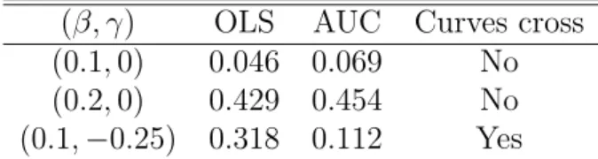
We also investigated for comparing two ROC curves, whether the OLS approach is more or less powerful than comparing the AUC values approach. Table 2 summaries the simulation results. We found that when two ROC curves cross, the OLS method is more powerful. But when the curves do not cross, AUC method is more powerful.
(Table 2 goes here)
3. Application to Pancreatic Cancer Data Set
This dataset was first published by Wieand et al.(1989). It is a case-control study including 90 cases with pancreatic cancer and 51 controls that did not have cancer but who had pancreatitis. Serum samples from each patient were assayed for CA-19-9, a carbohydrate antigen, and CA-125, a cancer antigen, both of which are measured on the continuous positive scale and higher values are more indicative of disease. A primary question to be addressed by the study is to determine which of the two biomarkers better distinguishes cases from controls. We will compare their corresponding ROC curves to address this question.
Since CA-125 and CA-19-9 are paired tests, we use the bootstrap variances in the in-ference. The distribution of the test results are closer to normal at the log scale, hence we calculated the correlation coefficients at that scale, which are -0.141 in the control group and 0.142 in the diseased group. Table 3 shows the parameter estimates when we compare the curves in the entire range of (0,1). Data is analyzed by letting g = Φ and using the boundary value (a, b)= (0.0001, 0.9999). We choose CA-125 to be test 1 and CA-19-9 to be test 2, therefore, (α0, α1) is the parameter for the CA-125 ROC curve, (α0+β, α1+γ) is the parameter for the CA-19-9 ROC curve and (β, γ) measures the difference between the two curves. After adjusting for multiple comparisons by Bonferroni method, we found the
p value for γ is 0.0067 < 0.025, but the p value for β is 0.0751 > 0.025, which means that the slopes of the two curves are statistically significantly different from each other but the intercepts of the two curves are not. The p value from the χ2 test is 0.0019, which shows
overall the curves are different. We also calculated the pvalue by comparing empirical AUC statistics, which is 0.007, hence we reach same conclusion by both method, but the pvalue from AUC-based test is larger, which can be explained by the fact that the two ROC curves have a cross in the end when t is close to 0.8, which is the setting when AUC-based test may not be as powerful as OLS-based test.
(Table 3 goes here)
Figure 1 shows the OLS-fitted ROC curves as well as the empirical curves for both CA-125 and CA-19-9. The fitted curves follows the empirical curves well, suggesting a good fitting.
(Figure 1 goes here)
Table 4 shows the parameter estimates when we are comparing only the part of curves when the false positive fraction is less than 20%. Data is analyzed by lettingg = Φ and using the boundary value (a, b)= (0.0001, 0.2). The p value forγ is slightly over 0.025(0.032) and the p value for β is not significant(p = 0.463). The p value from the χ2 test is p < 0.0001. The smaller p value here reflects the fact that the difference between the two curves are more prominent in the lower part of the curves.
(Table 4 goes here)
A test based on the difference in empirical partial AUC statistics found the differ-ence is statistically significantly different from 0 based on bootstrap distribution with p <
0.001(Pepe 2003). Again this p-value is slightly larger than the p-value based on the OLS method, suggesting the test based on the summary measure is not as powerful as the test based on comparing the actual curves. Figure 2 shows the OLS-fitted partial ROC curves as well as the empirical curves for both CA-125 and CA-19-9. The fitted curves follows the empirical curves well, suggesting a good fitting.
(Figure 2 goes here)
ROC-GLM method yields estimates for β = 0.23(se = 0.71) and γ = −0.91(se = 0.46)(Pepe 2000). Placement value regression method yields estimates for β = 0.02(se =
0.64) and γ = −0.98(se = 0.40)(Pepe & Cai 2002). Hence OLS method is more efficient than both ROC-GLM and PV regression methods. Notice although the estimates forβ and
γ are quite different across all three methods, because of the large se, those estimates are not inconsistent with each other.
To make conclusions about relative efficiency between the OLS method and the ROC-GLM method, we simulated data under the fitted model as shown in Table 3 where (α0, α1, β, γ) = (0.717, 0.986, 0.485, -0.518) and we chose the correlation coefficients to be the same as the values found in the pancreatic cancer data; ρ=−0.141 for the control group ρ= 0.142 for the diseased group. The simulation results suggested that the OLS estimator is more efficient than the ROC-GLM estimator under this setting. The variance for (ˆα0,αˆ1,β,ˆ γˆ) is (0.191, 0.130, 0.266, 0.162) for the OLS estimator and (0.193, 0.139, 0.269, 0.171) for the GLM estimator.
4. Modeling Covariate Effects
The covariates that potentially influence the test performance can be either categorical or continuous. Examples of categorical covariates include gender of the test subjects and dif-ferent test settings. Examples of continuous covariates include age of the test subjects. Although it is natural to model the covariate effects on its given scale, by modeling a contin-uous covariate, we usually make a stronger model assumption than modeling a categorical covariate.
To make this idea clear, consider the existing methodology to evaluate covariate effects on test performance using regression models for the ROC curve. The common feature for those methods is that they all assume a parametric model for the ROC curve. Those methods usually include the continuous covariates as linear terms, by doing that, they make an additional assumption that the ROC curves are “linearly” related, i.e. the tests are either getting progressively better or worse when the covariates values are getting larger. This is a pretty strong assumption and may not be appropriate for all covariates. For example, a test
may perform best in the young adults but not so good in children and elderly people. Hence the relationship between the test performance(ROC curve) and the age is not linear. By modeling the covariates as a categorical variable, however, we make less assumption about the directions of the covariates effect.
Although we argue here for the advantage of using categorical covariate in the model, interpretation from the model that uses continuous covariates is usually simpler. It is not our intention to discourage the use of continuous covariates in the model all together.
4·1 Uncorrelated versus Correlated Subsets
Suppose there are N categorical covariates available to us and we wish to include all of them in our model. Those covariates essentially partition the entire data into K subsets, each subset represents an unique combination of those N covariates. Those subsets could be correlated or uncorrelated. For example, when the covariate is the test setting and each individual receives tests under more than one setting, then the subsets would be correlated. If test results from those subsets are uncorrelated, this is analogous to the non-paired tests situation we discussed in the previous chapter. If, however, the test results from different subsets are correlated, we have “paired-tests” situation. Inference for uncorrelated and correlated subsets is a generalization of the inference for non-paired and paired tests, where in the latter case, the number of covariate is one and the number of subsets is two.
4·2 Regression Model for Covariate Effects
Assume there areN categorical covariates, resulting inK unique combination. Partition the data into the corresponding K subsets.
For subset 1(reference subset), assume
g−1(ROC
1(t)) = β1+γ1g−1(t) (14)
For subset k, k = 2, ..., K, assume
g−1(ROC
Hence βk is the difference in the intercept parameter of the ROC curves for subset k and
the reference subset and γk is the difference in the slope parameter of the ROC curves for
subset k and the reference subset.
The underlying assumptions for equation (14) is that there exists an unknown monotone increasing function h1, such that
h1(YD,¯ 1)∼N(0,1)
and
h1(YD,1)∼N(β1/γ1,1/γ12).
Similarly, for subsequent subset k, k= 2,3, ..., K, equation (15) assumes there exists an unknown monotone increasing function hk, such that
hk(YD,k¯ )∼N(0,1)
and
hk(YD,k)∼N((β1+βk)/(γ1+γk),1/(γ1+γk)2).
Notice that hks are not required to be the same for different k. The parameter we need to
estimate here is θ = (β1, γ1, ..., βK, γK)T. We can show in large samples, g−1(ROCd k(t)) for
k = 1,2, ...K are Gaussian processes,
√
nD,¯ 1(g−1(ROCd1(t))−g−1(ROC1(t))) −→D N(0,Σe,1) (16)
and
√
nD,k¯ (g−1(ROCdk(t))−g−1(ROCk(t)))−→D N(0,Σe,k) (17)
The proof of the above results and the definitions of Σe,1 and Σe,k can be found in Zhang
(2004).
4·3 Estimating Procedures Equation (16) and (17) imply g−1(ROC
k(t)) can be approximated by g−1(ROCd k(t)).
1. Follow the steps 1-5 from section 2.3 to calculate the pairs (tpk,ROCd (tpk)) for each
subset separately; 2. Let design matrix M be
M = M1 O O .. O M2 M2 O .. O M3 O M3 .. O . . . .. . MK O O .. MK (18) where M0 k= µ 1 ... 1 ... g−1(t 1,k) ... g−1(tpk) ... 
and O is a matrix with 0 in every entry. 3. Let ˜Y = ( ˜Y1,Y˜2, ...,Y˜K)T and ˜Yk = (g−1(ROCd (t1k))...g−1(ROCd (tpk)))T;
4. Our linear model is: for subset 1,
g−1(ROCd 1(tp,1))=. β1+γ1g−1(tp,1) +²1 (19)
where√nD,¯1²1 is normally distributed with mean 0 and asymptotic covariance matrix Σr,1;
For subset k, k = 2,3, ..., K
g−1(ROCd k(tp,k))=. β1+γ1g−1(tp,k) +βk+γkg−1(t) +²k (20)
where√nD,k¯ ²k is normally distributed with mean 0 and asymptotic covariance matrix
Σr,k;
5. Our OLS estimator for θ is
ˆ
θ = (M0M)−1M0Y˜ (21)
Asymptotic distribution theory for the OLS estimator when the subsets are not correlated is developed in Zhang(2004), in which the OLS estimator is shown to be unbiased and normally distributed. Asymptotic theory for the OLS estimator when the data are correlated needs to be developed in the future since joint asymptotic distribution for correlated multiple ROC curves is not yet available.
4·4 Covariate Consideration
We present our method by assuming all covariates are categorical. If we want to include continuous covariate Z in the model, we need to have ˆSD,Z¯ and ˆSD,Z for all possible values
of Z. Since it is impossible to do this non-parametrically, we are left with the choice of semiparametric and parametric modelling of ˆSD,Z¯ and ˆSD,Z. Semiparametric and parametric
modeling of ˆSD,Z¯ has been proposed by several authors(see Pepe(2003) for a comprehensive review), it is possible to impose a semiparametric or parametric model on ˆSD,Z as well. We
need to be more carefully here though, since for certain disease, the disease status makes the distribution of test results more irregular and unpredictable.
If certain covariate value is given on the continuous scale, we need to categorize it into appropriate groups first before applying OLS method. The categorization should depend on both the question of interest(i.e. scientific relevance) and the actual data, i.e., we need to make sure there are sufficient observations in each group. Based on our simulation studies, a sample size where the minimum of nD and nD¯ is at least 50 seems sufficient.
Least squares approach can also accomodate disease-specific covariates. For example, suppose there is a covariate for disease severity that has two categories: mild and severe. Then for each level of severity, we can just use the non-diseased observation as the reference population and calculate the corresponding T P F and F P F.
5. Application to DPOAE Data Set
The DPOAE data set was first published by Stover et.al (1996). DPOAE stands for dis-tortion product otoacoustic emission, which is an audiology test used to separate normal-hearing from normal-hearing-impaired ears. We only analyze a subset of the entire data set. The test is administrated under 9 different auditory stimulus conditions with three levels of fre-quency(1001, 1416 and 2002 Hz) and three levels of intensity(55, 60 and 65 dB SPL). A total of 210 subjects were included in the study. The subjects were considered cases with hearing impairment at a given frequency if their audiometric threshold exceeds 20dB HL measured
by a behaviour test(gold standard). Each subject was tested in only one ear. Test result is the negative signal-to-noise ratio, -SNR, with higher value being more indicative of hearing impairment. The objective of the analysis is to determine the optimal setting for the clinical use of DPOAE to separate normal from hearing-impaired ears, but bear in mind an ear may be determined to be hearing impaired or normal at different frequencies.
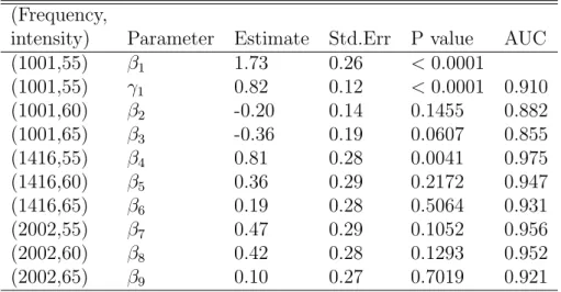
We partition the data into nine subsets, corresponding to the nine test settings. Since each subject is tested under more than one setting, those subsets are correlated, therefore we will use bootstrap method to estimate the variance. The bootstrap is done by sampling the subjects with replacement and use all the test results associated with each sampled subject. We apply the OLS method to the DPOAE data set using the models specified in (19) and (20). Data is analyzed by letting g = Φ and using the boundary value (a, b)= (0.0001, 0.9999). We choose the reference subset (subset 1) to be the test setting with frequency value of 1001Hz and intensity value of 55 dB SPL. The standard error is estimated from bootstrap method. (β1, γ1) is the intercept and slope estimates for the ROC curve for setting (1001, 55) and the subsequentβk and γk, withk = 2, ..,9, represent the differences in the intercept
and slope parameters of the ROC curves between subset k and subset 1. We found none of the ˆγk is statistically significantly different from 0 (P value> 0.5).
We also develop a χ2 test statistic ˆγ0ˆ
Σγˆγ, where γ = (γ2, ...γ9) and ˆΣγ is the estimated
covariance matrix of ˆγ. Write the null hypothesis as H0 : γ = 0 and compare the above statistic with a χ2 distribution with 8 degrees of freedom gives a P-value of 0.84, which is consistent with the result from testing the significance of each γk separately that the
interaction terms in model (4.2) are not statistically significant.
We re-analyze the data with the interaction terms omitted and Table 5 summarizes the results. From Table 5, we can see within the nine test settings, the setting (1416, 55) generates a ROC curve with the largest intercept estimate and the difference between it and the intercept estimate for the reference ROC curve (β4) is statistically significant with a P-value 0.0041. The P-value for other parameters(β2, β3, β5 to β9) are not significant.
The estimated ROC curve for setting (1416, 55) is ROC(t) = Φ(2.54 + 0.82Φ−1(t)) with estimated AUC value of 0.975, which is the largest among all settings. We know the larger the AUC value, the better the test in discrimating cases versus controls. From the sign of the estimates, we can see the performance of the test gets worse with the increasing intensity when we fix the frequency value. This analysis suggests (1416Hz, 55 dB SPL) is a better test setting than the reference setting.
(Table 5 goes here)
We have also analyzed the data by ROC-GLM method without the interaction terms and Table 6 summarizes the results.
(Table 6 goes here)
Table 5 and 6 show that OLS and ROC-GLM methods generate similar estimates for parameters β and γ. They have similar standard error estimates and inference based on either method is the same that both suggest setting (1416, 55) constitutes a better test than the reference setting (1001,55).
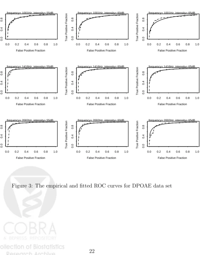
Figure 3 shows the empirical and the OLS-fitted ROC curves for all nine test settings. It shows the fitted ROC curves follows the empirical ROC curves very well, indicating good fittings.
(Figure 3 goes here)
6. Discussion
This manuscript addresses statistical methods to compare diagnostic tests performance and more generally, assess potential covariate effects on the test performance. Often a new developed test is being compared with an existing test to determine whether the new test has any advantage. If each individual in the population receives both tests, those tests are called paired tests; otherwise, they are called non-paired tests. We demonstrate how to use linear regression method(OLS) to compare ROC curves by assuming a parametric model for each curve and test the difference in the intercept and slope parameters of the curves. A
χ2 test statistic is developed under the regression framework to test the overall difference in the two curves. The asymptotic distribution theory for the OLS estimators is developed when the two tests are non-paired, in which the estimators are shown to be consistent and normally distributed asymptotically.
Summary measures like AUC or pAUC statistics can be used to compare two ROC curves as well. Although intuitive, this approach is underpowered in the situation when the two curves have cross-overs. Simulation studies are carried out to assess the size of the χ2 test as well as the size of the Z-test based on the empirical AUC statistics. We find both tests are slightly conservative in some cases but are suitable to be used in practice. We illustrate our method using the pancreatic cancer data set and find the two biomarkers are statistically significantly different from each other and CA-19-9 is a more accurate test. Standard error estimates for the OLS estimator is smaller than the estimates from other regression based methods when we compare partial ROC curves.
Various factors can affect a test performance beyond the disease status, which motivates incorporating the covariate information into the ROC curve analysis. We demonstrate how to use linear regression to estimate covariate effects. We illustrate our method on an audiology test(DPOAE) data set, in which we show that OLS and ROC-GLM estimators have similar standard error estimates in estimating the ROC curve parameters.
One topic left for comparing two ROC curves is the development of asymptotic theory for the OLS estimators when the two tests are paired. What is needed here is the joint distribution of two correlated empirical ROC curves. If shown that they have a bivariate normal distribution asymptotically, the asymptotic distribution theory for the OLS estimator can be approved easily.
For covariate effects modelling, we have only included categorical covariates in our linear regression model. We would like to explore whether continuous covariates can be accomo-dated in the model as well. One possible approach is for a given covariate Z, using either semiparametric or parametric model to model ˆSD,Z in addition to modeling ˆSD,Z¯ (Pepe,
2003).
In summary, the proposed linear regression framework provides an unified approach for the ROC curve analysis. It can be used to estimate or compare ROC curves, as well as incorporate covariate information in the model. The application of ROC curve goes beyond the medical diagnostic field and it can be used for evaluating any discrimination tools. It is, and will continue to be an important and exciting area to engage in research.
References
Metz, C. E., Herman, B. A., and Shen, J. H. (1998), “Maximum likelihood estimation of receiver operating characteristic (ROC) curves from continuously-distributed data” Statistics in Medicine, 17, 1033–1053.
Metz, C. E., and Kronman, H. B. (1980), “Statistical significance tests for binormal roc curves”Journal of Mathematical Psychology, 22, 218–243.
Pepe, M. S. (1997), “A regression modelling framework for receiver operating characteristic curves in medical diagnostic testing,” Biometrika, 84, 595–608.
Pepe, M. S. (2000), “An interpretation for the ROC curve and inference using GLM proce-dures” Biometrics, 56(2), 352–359.
Pepe, M. S. (2003), “The statistical evaluation of medical tests for classification and predic-tion”, Oxford University Press, United Kingdom.
Pepe, M. S., and Cai, T. (2004), “The analysis of placement values for evaluating discrimi-natory measures” Biometrics, 60, 528–535.
Stover, L., Gorga, M. P., Neely, S. T. and Montoya, D. (1996), “Toward optimizing the clinical utility of distortion product otoacoustic emission measurements” Journal of the Acoustic Society of America, 100, 956–967.
Wieand, S., Gail, M. H., James, B. R. and James, K. L. (1989), “A family of nonparametric statistics for comparing diagnostic markers with paired or unpaired data”Biometrika, 76, 585–592.
Zhang, Z. (2004), ”Semiparametric least squares analysis of the receiver operating charac-teristic curve” University of Washington Doctoral Dissertation.
Table 1: Rejection rates and confidence intervals forχ2 test based on the OLS estimator and Z-test based on the empirical AUC statistics. Results are based on 500 simulation runs.
ρ χ2 test Z-test
0 4.8%(2.9%,6.7%) 3.2%(1.7%,4.7%) 0.25 3.2%(1.7%,4.7%) 6.4%(4.3%,8.5%) 0.5 5.0%(3.1%,6.9%) 6.0%(3.9%,8.1%) 0.75 5.0%(3.1%,6.9%) 5.4%(3.4%,7.4%)
Table 2: Power of the OLS method and the AUC method. Results are based on 1000 simulation runs. (α0, α1)=(0.5,0.75) andρ= 0.
(β, γ) OLS AUC Curves cross (0.1,0) 0.046 0.069 No (0.2,0) 0.429 0.454 No (0.1,−0.25) 0.318 0.112 Yes
Table 3: Comparison of the whole ROC curves for CA-19-9 and CA-125 from the pancreatic cancer data set by the OLS method.
Parameter Estimate SE(bootstrap) P value
α0 0.717 0.206 0.0005
α1 0.986 0.165 <0.0001
β 0.485 0.273 0.0751
γ -0.518 0.191 0.0067
Table 4: Comparison of the partial ROC curves for CA-19-9 and CA-125 when the false positive fractions are below 20%.
Parameter Estimate SE(bootstrap) P value
α0 0.594 0.565 0.293
α1 1.030 0.306 0.0008
β 0.455 0.619 0.463
Table 5: Covariates effects on the ROC curves estimated by the the OLS method for the DPOAE test.
(Frequency,
intensity) Parameter Estimate Std.Err P value AUC (1001,55) β1 1.73 0.26 <0.0001 (1001,55) γ1 0.82 0.12 <0.0001 0.910 (1001,60) β2 -0.20 0.14 0.1455 0.882 (1001,65) β3 -0.36 0.19 0.0607 0.855 (1416,55) β4 0.81 0.28 0.0041 0.975 (1416,60) β5 0.36 0.29 0.2172 0.947 (1416,65) β6 0.19 0.28 0.5064 0.931 (2002,55) β7 0.47 0.29 0.1052 0.956 (2002,60) β8 0.42 0.28 0.1293 0.952 (2002,65) β9 0.10 0.27 0.7019 0.921
Table 6: Covariates effects on the ROC curves estimated by the ROC-GLM method for the DPOAE test.
(Frequency,
intensity) Parameter Estimate Std.Err P value (1001,55) β1 1.84 0.29 <0.0001 (1001,55) γ1 0.95 0.13 <0.0001 (1001,60) β2 -0.21 0.13 0.1097 (1001,65) β3 -0.32 0.19 0.1029 (1416,55) β4 0.82 0.30 0.0073 (1416,60) β5 0.39 0.31 0.2022 (1416,65) β6 0.18 0.30 0.5436 (2002,55) β7 0.41 0.28 0.1496 (2002,60) β8 0.46 0.29 0.1082 (2002,65) β9 0.06 0.27 0.8221
False Positive Fraction
True Positive Fraction
0.0 0.2 0.4 0.6 0.8 1.0 0.0 0.2 0.4 0.6 0.8 1.0 Top: CA-19-9 Bottom: CA-125
Figure 1: The OLS-fitted ROC curves along with the empirical curves for 125 and CA-19-9
False Positive Fraction
True Positive Fraction
0.0 0.05 0.10 0.15 0.20 0.0 0.2 0.4 0.6 0.8 1.0 Top: CA-19-9 Bottom: CA-125
Figure 2: The OLS-fitted partial ROC curves along with the empirical curves for CA-125 and CA-19-9
False Positive Fraction
True Positive Fraction
0.0 0.2 0.4 0.6 0.8 1.0
0.0
0.4
0.8
frequency= 1001Hz, intensity= 55dB
False Positive Fraction
True Positive Fraction
0.0 0.2 0.4 0.6 0.8 1.0
0.0
0.4
0.8
frequency= 1001Hz, intensity= 60dB
False Positive Fraction
True Positive Fraction
0.0 0.2 0.4 0.6 0.8 1.0
0.0
0.4
0.8
frequency= 1001Hz, intensity= 65dB
False Positive Fraction
True Positive Fraction
0.0 0.2 0.4 0.6 0.8 1.0
0.0
0.4
0.8
frequency= 1416Hz, intensity= 55dB
False Positive Fraction
True Positive Fraction
0.0 0.2 0.4 0.6 0.8 1.0
0.0
0.4
0.8
frequency= 1416Hz, intensity= 60dB
False Positive Fraction
True Positive Fraction
0.0 0.2 0.4 0.6 0.8 1.0
0.0
0.4
0.8
frequency= 1416Hz, intensity= 65dB
False Positive Fraction
True Positive Fraction
0.0 0.2 0.4 0.6 0.8 1.0
0.0
0.4
0.8
frequency= 2002Hz, intensity= 55dB
False Positive Fraction
True Positive Fraction
0.0 0.2 0.4 0.6 0.8 1.0
0.0
0.4
0.8
frequency= 2002Hz, intensity= 60dB
False Positive Fraction
True Positive Fraction
0.0 0.2 0.4 0.6 0.8 1.0
0.0
0.4
0.8
frequency= 2002Hz, intensity= 65dB