Marc van Kreveld
a, Bettina Speckmann
b,∗aInstitute for Information and Computing Sciences, Utrecht University, The Netherlands bDepartment of Mathematics and Computer Science, TU Eindhoven, The Netherlands Received 1 May 2004; received in revised form 15 January 2005; accepted 15 June 2006
Available online 18 September 2006 Communicated by C. Cortes and A. Marquez
Abstract
A rectangular cartogram is a type of map where every region is a rectangle. The size of the rectangles is chosen such that their ar-eas represent a geographic variable (e.g., population). Good rectangular cartograms are hard to generate: The area specifications for each rectangle may make it impossible to realize correct adjacencies between the regions and so hamper the intuitive understanding of the map.
We present the first algorithms for rectangular cartogram construction. Our algorithms depend on a precise formalization of region adjacencies and build upon existing VLSI layout algorithms. Furthermore, we characterize a non-trivial class of rectangular subdivisions for which exact cartograms can be computed efficiently. An implementation of our algorithms and various tests show that in practice, visually pleasing rectangular cartograms with small cartographic error can be generated effectively.
©2006 Elsevier B.V. All rights reserved. Keywords:Cartogram; Rectangular layout
1. Introduction
Cartograms. Cartograms are a useful and intuitive tool to visualize statistical data about a set of regions like countries, states or counties. The size of a region in a cartogram corresponds to a particular geographic variable. The most common variable is population: in a population cartogram, the sizes (measured in area) of the regions are proportional to their population. In fact, a cartogram is actually able to visualize more than one geographic variable at a time: it can depict a second geographic variable by shades of color [6,18]. Cartograms are also calledvalue-by-area maps.
In a cartogram the sizes of the regions are not the true sizes and hence the regions generally cannot keep both their shape and their adjacencies. A good cartogram, however, preserves the recognizability in some way. Globally speaking, there are four types of cartogram. The standard type—also referred to as contiguous area cartogram—has de-formed regions so that the desired sizes can be obtained and the adjacencies kept. Algorithms for such cartograms were given, among others, by Tobler [23], Dougenik et al. [8], Kocmoud and House [15], Edelsbrunner and Waupotitsch [9],
* Corresponding author.
E-mail addresses:[email protected] (M. van Kreveld), [email protected] (B. Speckmann). 0925-7721/$ – see front matter ©2006 Elsevier B.V. All rights reserved.
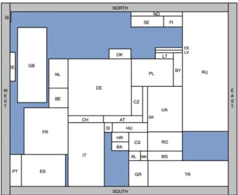
Fig. 1. The population of Europe (country codes according to the ISO 3166 standard).
Keim et al. [14], and Gastner and Newman [11]. The second type of cartogram is the non-contiguous area cartogram [10,19]. The regions have the true shape, but are scaled down and generally do not touch anymore. Sometimes the scaled-down regions are shown on top of the original regions for recognizability. A third type of cartogram is based on circles and was introduced by Dorling [7]. The fourth type of cartogram is the rectangular cartogram in-troduced by Raisz in 1934 [21]. Each region is represented by a single rectangle, which has the great advantage that the sizes (area) of the regions can be estimated much better than with the first two types. However, the rectangu-lar shape is less recognizable and it imposes limitations on the possible layout. Hybrid cartograms of the first and fourth type exist as well. There regions are rectilinear polygons with a small number of vertices instead of rectan-gles.
Quality criteria. Whether a rectangular cartogram is good is determined by several factors. One of these is the cartographic error[8,9], which is defined for each region as|Ac−As|/As, whereAcis the area of the region in the cartogram andAsis the specified area of that region, given by the geographic variable to be shown. The following list summarizes all quality criteria:
• Average and maximum cartographic error.
• Correct adjacencies of the rectangles (e.g., the rectangles for Germany and France should be adjacent and the rectangles for Germany and Spain should not be adjacent).
• Maximum aspect ratio.
• Suitable relative positions (e.g., the rectangle for The Netherlands should be West of the one for Ger-many).
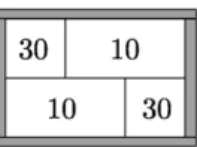
For a purely rectangular cartogram we cannot expect to simultaneously satisfy all criteria well. Fig. 2 shows an example where correct adjacencies must be sacrificed in order to get a small cartographic error. In larger examples, bounding the aspect ratio of the rectangles also results in larger cartographic error.
Related work. Rectangular cartograms are closely related tofloor plansfor electronic chips and architectural de-signs. Floor planning aims to represent a planar graph by its rectangular dual, defined as follows. Arectangular partitionof a rectangleR is a partition ofR into a setSof non-overlapping rectangles such that no four rectangles inS meet at the same point. Arectangular dualof a plane graphGis a rectangular partitionR, such that (i) there is a one-to-one correspondence between the rectangles inRand the nodes inG, and (ii) two rectangles inRshare a common boundary if and only if the corresponding nodes inGare connected. Atriangleis a cycle ofGconsisting of three arcs (a 3-cycle). A cycleCofGdivides the plane into an interior and an exterior region. IfC contains at least one vertex in its interior and in its exterior thanC is called aseparating cycle. The following theorem was proven in [2,16]:
Fig. 2. The values inside the rectangles indicate the preferred areas.
Theorem 1.A plane graphGhas a rectangular dualRwith four rectangles on the boundary ofRif and only if (1) every interior face is a triangle and the exterior face is a quadrangle
(2) Ghas no separating triangles.
Planar graphs that do not have a rectangular dual can still be represented by using other shapes than rectangles. It was shown in [17] that L- and T-shapes in addition to rectangles are always sufficient to represent a planar graph. A rectangular dual is not necessarily unique.
Although every triangulated planar graph without separating triangles and a quadrangle as the exterior face has a rectangular dual this does not imply that an error free cartogram for this graph exists. The area specification for every rectangle, as well as other criteria for good cartograms, may make it impossible to realize. Only a careful trade-off between the various types of errors (for example incorrect areas or incorrect adjacencies) makes it possible to visualize certain data sets as rectangular cartograms.
The only algorithm for standard cartograms that can be adapted to handle rectangular cartograms is Tobler’s pseudo-cartogram algorithm [23] combined with a rectangular dual algorithm. Tobler’s pseudo-cartogram algorithm starts with an orthogonal grid superimposed on the map, after which the horizontal and vertical lines of the grid are moved to stretch and shrink the strips in between. Hence, if the input to Tobler’s algorithm is a rectangular partition, then the output is also a rectangular partition. However, Tobler’s method is known to produce a large cartographic er-ror and is mostly used as a preprocessing step for cartogram construction [18]. Furthermore, Tobler himself in a recent survey [24] states that none of the existing cartogram algorithms are capable of generating rectangular cartograms.
A few other papers exist that discuss constructions related to rectangular cartograms. Biedl and Genc [3] show NP-hardness of certain orthogonal layout problems with prescribed areas, while Heilmann et al. [12], Rahman et al. [20], and de Berg et al. [5] provide algorithms to construct rectangular or orthogonal layouts with prescribed areas. It is unknown whether the computation of rectangular cartograms with correct adjacencies and no error is NP-hard.
Results. We present the first algorithms for the computation of rectangular cartograms. We formalize the region ad-jacencies based on their geographic location and use this information to construct a rectangular subdivision. The steps that lead us from the input data to an algorithmically processable rectangular subdivision are described in Section 2.
We describe three algorithms that compute a cartogram from a rectangular subdivision. The first is an easy and efficient heuristic which we evaluated experimentally. The visually pleasing results of our implementation (which compare favorably with existing hand-drawn or computer assisted cartograms) can be found in Section 6. Secondly, we show how to formulate the computation of a cartogram as a bilinear programming problem (see Section 5).
For our third algorithm we introduce an effective generalization of sliceable layouts, namelyL-shape destructible layouts. We prove in Section 3 that the coordinates of an L-shape destructible layout are uniquely determined by the specified areas (if an exact cartogram exists at all for a specific set of area values). The proof immediately implies an efficient algorithm to compute an exact (up to an arbitrarily small error) cartogram for subdivisions that arise from actual maps.
2. Algorithmic outline
Assume that we are given an administrative subdivision into a set of regions. The regions and adjacencies can be represented by nodes and arcs of a graphF, which is the face graph of the subdivision.
1.Preprocessing: To satisfy the conditions of Theorem 1 we have to ensure that the face graphF is triangulated and contains no internal nodes of degree less than four.F is in most cases already triangulated (except for its outer face). We triangulate any remaining non-triangular faces (for example the face formed by the nodes for Nevada, Utah,
New Mexico, and Arizona). Our algorithms consider every possible triangulation of non-triangular faces, since each triangulation leads to a different rectangular dual.
It remains to preprocess internal nodes of degree less than four. There are several places on a country map of the world where a country does not have enough neighbors to allow rectangular faces only. For example, Luxembourg is adjacent only to Belgium, Germany, and France. Hence, in the adjacency graph, Belgium, Germany, and France form a separating triangle that separates Luxembourg from the other European countries. In this case, the most reasonable solution is to treat the union of Belgium and Luxembourg as a single region with summed area value and later decide which part of the lower right should be the rectangle for Luxembourg. Belgium will become L-shaped. Similar examples on the world map are Paraguay, Malawi, and Burundi.
Another problem are countries adjacent to only two other countries. These two adjacent countries must then have two adjacencies, one to either side of the country which they enclose. Examples are Mongolia, Andorra, Nepal, Moldova, and Bhutan. In these cases we also remove the 2-adjacency country from the map and add its area to one of its neighbors. It will be inserted as a rectangle inside that neighbor after the rectangular cartogram algorithm has finished. The neighbor will become C-shaped. There is no guarantee that the insertion can preserve the correct adjacencies and areas.
Yet another problem are countries that are surrounded completely by one neighbor. Examples are Lesotho inside South Africa and the Bundesland Berlin inside Brandenburg. This case is easy to handle: we add the area of the country to its only neighbor, run the rectangular cartogram algorithm, and insert a rectangle of the correct size in the middle. The surrounding country will become O-shaped.
Finally, there are cases where regions are disconnected, like the Bundesland Bremen in Germany. We can choose one of its components to be its representative in the rectangular cartogram.
2.Directed edge labels: Any two nodes in the face graph have at least one direction of adjacency which follows naturally from their geographic location (for example, The Netherlands lies clearly West of Germany). While in theory there are four different directions of adjacency any two nodes can have, in practice only one or two directions are reasonable (for example, Germany can be considered to lie West or North of Austria). We employ a simple heuristic to extract the possible directions of adjacency from the administrative subdivision: we consider the line through the centers of mass of the two regions and let its orientation determine the directions.
Our algorithms go through all possible combinations of direction assignments and determine which one gives a correct or the best result. While in theory there can be an exponential number of options, in practice there is often only one natural choice for the direction of adjacency between two regions. We call a particular choice of adjacency directions adirected edge labeling.
Observation 1.A face graphF with a directed edge labeling can be represented by a rectangular dual if and only if (1) every internal region has at least one North, one South, one East, and one West neighbor;
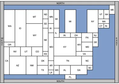
(2) when traversing the neighbors of any node in clockwise order starting at the western most North neighbor we first encounter all North neighbors, then all East neighbors, then all South neighbors and finally all West neighbors. For example, a realizable directed edge labeling for the US cannot let Nevada have California to the West, Oregon and Idaho to the North, and Utah and Arizona to the East, because then Nevada would miss a South neighbor.
A realizable directed edge labeling constitutes aregular edge labelingforF as defined in [13] which immediately implies our observation.
3.Rectangular layout: To actually represent a face graph together with a realizable directed edge labeling as a rectangular dual we have to pay special attention to the nodes on the outer face since they may miss neighbors in up to three directions. To compensate for that we add four special regions NORTH, EAST, SOUTH, and WEST, as well assea regionsthat help to preserve the original outline of the subdivision. Then we can employ the algorithm by He and Kant [13] to construct arectangular layout, i.e., the unique rectangular dual of a realizable directed edge labeling. The output of our implementation of the algorithm by He and Kant is shown in Fig. 3.
4.Area assignment: For a given set of area values and a given rectangular layout we would like to decide if an assignment of the area values to the regions is possible without destroying the correct adjacencies. If the answer is negative or if a solution cannot be found, then we still want to compute a cartogram that has a small cartographic error while maintaining reasonable aspect ratios and relative positions.
Fig. 3. One of 4608 possible rectangular layouts of the US.
Fig. 4. Rectangular layout of the 12 provinces of the Netherlands and a corresponding maximal rectangle hierarchy.
In this paper we introduce and discuss three methods for computing cartograms from rectangular layouts. We implemented (parts of) our algorithms and we present experimental results in Section 6. In the remainder of this section we give a short overview of our algorithms.
Segment moving heuristic. A simple but efficient heuristic: We iteratively move horizontal and vertical segments of the rectangular layout to reduce the maximum relative error. Additional details can be found in Sections 4 and 6.
Bilinear programming. The computation of a cartogram with the correct adjacencies and minimum relative er-ror can be formulated as a bilinear programming problem, which unfortunately is nonconvex. Nevertheless, some non-linear programming methods may still be able to solve certain instances of the problem because the number of variables and constraints is only linear in the number of rectangles. Additional details can be found in Section 5.
L-sequence algorithm. For arbitrary layouts it is currently unknown if one can decide in polynomial time if an exact cartogram exists. But for certain types of rectangular layouts we can compute an exact or nearly exact cartogram. We first determine for a given rectangular layout amaximal rectangle hierarchy. The maximal rectangle hierarchy groups rectangles that together form a larger rectangle, as illustrated in Fig. 4. It can be computed in linear time [22]. All groups in the hierarchy are independent and we will determine areas separately for each group.
A node of degree 2 in the hierarchy corresponds to a sliceable group of rectangles. If the maximal rectangle hierarchy consists of slicing cuts only, then we can (in a top-down manner) compute the unique position of each slicing cut. Here we may introduce wrong adjacencies, but this will only happen if there is no correct rectangular cartogram.
Nodes of a degree higher than 2 (which is necessarily at least 5) require more complex cuts (see for example the four thick segments in Fig. 4). One of the main contributions of this paper is the characterization of a type of non-sliceable layout for which the coordinates are still uniquely determined by the specified areas. We describe an efficient algorithm to compute a cartogram forL-shape destructiblelayouts (see Section 3 for a precise definition). L-shape destructible layouts are a natural generalization of sliceable layouts with a clear practical value. For example, the rectangular layout of the 48 contiguous states of the US depicted in Fig. 3 is not sliceable, but it is L-shape
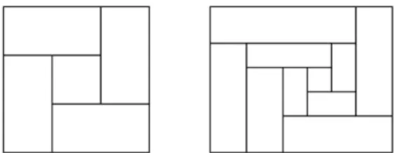
Fig. 5. Smallest non-sliceable layout (left), smallest non-L-shape destructible layout (right).
Fig. 6. An L-shape destructible layout of the Eastern US. The shaded area shows the L-shaped polygon after the removal of rectangles 1–4. destructible. If an L-shape destructible group exists in the maximal rectangle hierarchy, its unique area assignment is used for the cartogram. Wrong adjacencies between rectangles of different groups can occur, but only if no correct cartogram exists.
Fig. 5 shows the smallest non-sliceable layout, as well as the smallest non-L-shape destructible layout. In Section 3 we show that it is difficult to analytically solve the equations that arise from L-shape destructible layouts. But it is possible to produce a cartogram based on one guessed value (coordinate) and decide whether the initial choice was too large or too small in linear time.
3. L-shape destructible layouts
In this section we show that for certain non-sliceable rectangular layouts we can determine an exact or nearly exact rectangular cartogram efficiently (if one exists). Recall that a rectangular layoutRis a partition of a rectangleRinto a setSof non-overlapping rectangles such that no four meet in a point. We call a rectangular layoutRirreducibleif no proper subset ofS(of size>1) forms a rectangle. Furthermore, we call a rectilinear simple polygon with at most 6 verticesL-shaped.
Definition 2(L-shape destructible).An irreducible rectangular layoutRof a rectangleRisL-shape destructibleif a sequenceR1, R2, . . . , Rnof the rectangles inRexists such that rectangleR1is incident to a cornersofR, rectangle
Rnis incident to the cornertofRopposite tos, and for each 1i < n, the polygonR\ {R1, . . . , Ri}is an L-shaped polygon.
Fig. 8. An L-shape destructible layout. Fig. 9. Setting the height of the first rectangle in an L-shape destruction sequence. Note that the removal sequence is not necessarily unique. However, an incremental algorithm cannot make a bad decision, so the sequence can easily be computed in linear time. See Fig. 6 for an example of a removal sequence for an irreducible layout obtained from the maximal rectangle hierarchy of the rectangular layout of the Eastern United States depicted in Fig. 3.
The easiest type of non-sliceable but L-shape destructible layouts arewindmilllayouts (see Fig. 7;x1,x2, andx3 arex-coordinates of vertical segments andy1andy2arey-coordinates of horizontal segments). For a given set of area values{A1, . . . , A5}we can compute the (unique) realization analytically because this only requires finding roots of a polynomial of degree 2. We can scale the axes of any instance such that the outer rectangle has coordinates(0,0), (0,1),(A,0), and(A,1), whereA=A1+A2+A3+A4+A5. Then we get the five equations
x1·y1=A1
x2·(1−y1)=A2
(x2−x1)·(y1−y2)=A3
(x3−x1)·y2=A4
(x3−x2)·(1−y2)=A5 where alsox3=A.
Solving these equations with respect to, say,y1, we obtain a quadratic equation iny1. A windmill layout always has a realization as a cartogram, independent of the area values, which follows from the proof of Theorem 3.
Already for only slightly more complex types, for example Fig. 8, we cannot determine the coordinates exactly anymore, because this requires finding the roots of a polynomial of degree 6. Although the degree of the polynomials suggests that there may be more than one solution, we show that every L-shape destructible layout has at most one unique realization as a cartogram for a given set of area values. Furthermore we can compute the coordinates of this realization with an easy, iterative method.
Theorem 3.An L-shape destructible layout with a given set of area values has exactly one or no realization as a cartogram.
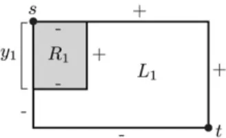
Proof. Without loss of generality we assume that the L-shape destruction sequence begins with a rectangleR1that contains the upper left corner ofR. We denote the height ofR1withy1(see Fig. 9) and the L-shaped polygon that remains after the removal ofR1byL1.
If we consider the edge lengths of L1 to be a function of y1 then we observe that these functions are either monotonically increasing iny1(denoted by a plus sign near the edge) or monotonically decreasing iny1(denoted by a minus sign near the edge). This is true because the area ofR1is specified. (Note here that the length of the right and bottom edges in Fig. 9 is actually fixed. We simply declare them to be monotonically increasing and decreasing respectively.) In fact, we will prove a much stronger statement: The lengths of the edges of the L-shaped polygons remaining after each removal of a rectangle in an L-shape reduction sequence are monotone functions iny1.
Clearly this statement is true after the removal ofR1.L1is of the L-shape type depicted in the upper left corner of Fig. 10. We will now argue by means of a complete case analysis that during a destruction sequence only L-shaped polygons of the three types depicted in the left column of Fig. 10 can ever occur. Note that the type of an L-shaped polygon also specifies which of its edges are monotonically increasing or decreasing iny1.
For each type of L-shaped rectangle there is only a constant number of possible successors in the destruction sequence, all of which are depicted in Fig. 10. We invite the reader to carefully study this figure to convince him or
Fig. 10. Removing a rectangle from an L-shaped polygon. The plus and minus signs next to an edge indicate that its length is a monotonically increasing or monotonically decreasing function ofy1.
herself that it indeed covers all possibilities. Note that we never need to know exactly which functions describe the edge lengths of the L-shaped polygons—it is sufficient to know that they are always monotone iny1.
During the destruction sequence it is possible that we realize that our initial choice ofy1 was incorrect. Every rectangleRi should be placed according to exactly one of the layouts depicted in Fig. 10. If the area ofRi is too large or too small for it to be placed in the proper layout then we can infer from the signs of the edges whethery1 needs to be increased or decreased to achieve correct adjacencies. For example, assume that a rectangleRi should be placed according to the layout of the second case of the top row of Fig. 10 but its area is too small and it would in fact be placed according to the layout of the first case of the top row. Then the signs of the edges show thaty1must be increased to obtain correct adjacencies. Should no further increase ofy1be possible, then we know that the correct adjacencies can not be realized for this particular layout and area values. All other cases can be treated in a similar manner.
If the choice ofy1does not give incorrect adjacencies during the rectangle placements up to the last ones, we can still decide whethery1should be larger or smaller, when we try to place the last rectangles. Ify1has the correct value, all rectangles fit perfectly intoR. Otherwise, one of the rectangles (the second to last rectangle, or some rectangle before) that should extend exactly to the right or bottom edge ofR, will either stick out beyond this edge ofR, or will not stick out far enough to reach it. This tells us whethery1should be chosen smaller or larger.
A binary search ony1 either leads to a unique solution or we recognize that the rectangular layout cannot be realized as a cartogram with correct areas. 2
4. Segment moving heuristic
A very simple but effective heuristic to obtain a rectangular cartogram from a rectangular layout is the following. Consider the maximal vertical segments and maximal horizontal segments in the layout, for example the vertical segment in Fig. 3 that has Kentucky (KY) to its left and West Virginia (WV) and Virginia (VA) to its right. This segment can be moved a little to the left, making Kentucky smaller and the Virginias larger, or it can be moved to the right with the opposite effect.
The segment moving heuristic loops over all maximal segments and moves each with a small step in the direction that decreases the maximum error of the adjacent regions. After a number of iterations, one can expect that all maximal segments have moved to a locally optimal position. However, we have no proof that the method reaches the global optimum or that it even converges.
The segment moving heuristic has some important advantages: (i) it can be used for any rectangular layout, (ii) one iterative step for all maximal segments takes O(n)time, (iii) no area needs to be specified for sea rectan-gles, (iv) a bound on the aspect ratio can be specified, and (v) adjacencies between the rectangles can be preserved, but need not be. Not preserving adjacencies can help to reduce cartographic error.
Fig. 11. A cartogram depicting the electricity production of Europe.
To preserve adjacencies, we have to make sure that two vertical segments incident to the same horizontal segment do not swap inx-order. For example, the vertical segment between Kentucky and the Virginias (Fig. 3) should not go further left than the segment bounding Kentucky to its left, but also no further than the segment between Indiana and Ohio. Otherwise, Indiana and West Virginia become adjacent. In this case we still have a rectangular partition, but it yields a rectangular cartogram with false adjacencies. We examine the cartograms produced by the segment moving heuristic with correct and false adjacencies in Section 6.
5. Bilinear programming
Once a rectangular layout is fixed, the rectangular cartogram problem can be formulated as an optimization prob-lem. The variables are thex-coordinates of the vertical segments and they-coordinates of the horizontal segments. For proper rectangular layouts (no four-rectangle junctions, inside an outer rectangle) withnrectangles, there aren−1 variables. The area of each rectangle is determined by four of the variables.
We can formulate the minimum error cartogram problem as a bilinear program: the rectangle constraints for a rectangleRare:
(xj−xi)·(yl−yk)(1−)·AR, (xj−xi)·(yl−yk)(1+)·AR
wherexi andxjare thex-coordinates of the left and right segment,ykandylare they-coordinates of the bottom and top segment,ARis the specified area ofR, andis the cartographic error forR. An additional O(n)linear constraints are needed to preserve the correct adjacencies of the rectangles (e.g., along sliceable cuts). Also, bounded aspect ratio (height-width) of all rectangles can be guaranteed with linear constraints. The objective function is to minimize. The formulation is a quadratic programming problem with quadratic constraints that include non-convex ones, and a linear optimization function. Since there are noxi2oryj2terms, onlyxiyjterms, it is a bilinear programming problem. Several approaches exist that can handle such problems, but they do not have any guarantees [1].
6. Implementation and experiments
We have implemented the segment moving heuristic and tested it on several data sets. The main objective was to discover whether rectangular cartograms with reasonably small cartographic error exist, given that they are rather restrictive in the possibilities to represent all rectangle areas correctly. Obviously, we can only answer this question if the segment moving heuristic actually finds a good cartogram if it exist. Secondary objectives of the experiments are to determine to what extent the cartographic error depends on maximum aspect ratio and correct or false adjacencies. We were also interested in the dependency of the error on the percentage of area used by the sea.
Table 1
Errors for different aspect ratios and sea percentages (correct adjacencies)
Data set Sea Aspect ratio Ave. error Max. error
Europe elec. 20% 8 0.071 0.280 Europe elec. 20% 9 0.070 0.183 Europe elec. 20% 10 0.067 0.179 Europe elec. 20% 11 0.065 0.155 Europe elec. 20% 12 0.054 0.137 Europe elec. 10% 10 0.098 0.320 Europe elec. 15% 10 0.076 0.245 Europe elec. 20% 10 0.067 0.179 Europe elec. 25% 10 0.049 0.126 Table 2
Errors for different aspect ratios, and correct or false adjacencies. Sea 20%
Data set Adjacency Aspect ratio Ave. error Max. error
US population false 8 0.104 0.278 US population false 9 0.085 0.193 US population false 10 0.052 0.295 US population false 11 0.030 0.091 US population false 12 0.022 0.056 US population correct 12 0.327 0.618 US population correct 13 0.319 0.608 US population correct 14 0.317 0.612 US population correct 15 0.314 0.569 US population correct 16 0.308 0.612 US highway correct 6 0.073 0.188 US highway correct 7 0.059 0.111 US highway correct 8 0.058 0.101 US highway correct 9 0.058 0.101 US highway correct 10 0.058 0.101
Our layout data sets consist of the 36 countries of Europe, and the 48 contiguous states of the USA. For Europe, we joined Belgium and Luxembourg, and Ukraine and Moldova, because rectangular duals do not exist if Luxembourg or Moldova are included as a separate country. Europe has 16 sea rectangles and the US data set has 9. For Europe we allowed 10 pairs of adjacent countries to be in different relative position, leading to 1024 possible layouts. Of these, 768 correspond to a realizable directed edge labeling. For the USA we have 13 pairs, 8192 possible layouts, and 4608 of these are realizable. In the experiments, all 768 or 4608 layouts are considered and the one giving the lowest average error is chosen as the cartogram.
As numeric data we considered for Europe thepopulation and theelectricity production, taken from [4]. For the USA we consideredpopulation,native population, number offarms, and total length ofhighways. The data is provided by the US census bureau in theStatistical Abstract of the United States.1
We used integer coordinates for all segments, and used steps of size 1 to move a segment. For the USA the outer rectangle has size 600 by 400, for Europe this is 500 by 400. In all our tests, no more than 400 iterations over all segments were needed until no more improvement could be made by a single move.
Our tests on the data sets showed that the false adjacency option always gives considerably lower error than correct adjacencies. The false adjacency option always allowed cartograms with average error of only a few percent. A small part of the errors is due to the discrete steps taken when moving the segments. Since cartograms are interpreted
Fig. 12. A cartogram depicting the native population of the United States.
Fig. 13. The population of the US.
visually and show a global picture, errors of a few percent on the average are acceptable. Errors of a few percent are also present in standard, computer-generated contiguous cartograms [8,9,14,15]. We note that hand-made rectangular cartograms also have false adjacencies and that aspect ratios of more than 20 can be observed ([4] and older editions). Table 1 shows errors for various settings for the electricity production data set. The rectangular layout chosen for the table is the one with lowest average error. The corresponding maximum error is shown only for completeness. In the table we observe that the error goes down with a larger allowed aspect ratio, as expected. For Europe and population (not shown in the table), errors below 0.1 on the average with correct adjacencies were only obtained for aspect ratios greater than 15. The table also shows that a larger sea percentage brings the error down. This is as expected because sea rectangles can grow or shrink to reduce the error of adjacent countries, while a sea rectangle cannot have an error in its area. So, more sea means more freedom to reduce errors. However, sea rectangles should not become so small that they visually (nearly) disappear.
Table 2 shows errors for various settings for two US data sets. Again, we choose the rectangular layout giving the lowest average error. In the US highway data set, aspect ratios above 8 do not seem to decrease the error below a certain value. In the US population data set, correct adjacencies give a larger error than is acceptable. Even an aspect ratio of 40 gave an average error of over 0.3. We ran the same tests for the native population data and again observed that the error decreases with larger aspect ratio. An aspect ratio of 7 combined with false adjacency gives a cartogram
Fig. 14. The highway kilometers of the US.
Fig. 15. The farms of the US.
with average error below 0.04 (see Fig. 12). Only the highways data allowed correct adjacencies, small aspect ratio, and small error simultaneously.
Figs. 12, 13, 14, and 15 show rectangular cartograms of the US. Three of them have false adjacencies, but we can observe that adjacencies are only slightly disturbed in all cases (which is the same as for the hand-made rectangular cartograms in [4]). The data sets allowed an aspect ratio of 10 or lower to yield an average error between 0.03 and 0.06, except for the farms data. Here an aspect ratio of 20 gives an average error of just below 0.1. Figs. 1 and 11 show rectangular cartograms for Europe. The former has false adjacencies and aspect ratio bounded by 12, the latter has correct adjacencies and aspect ratio bounded by 8. The average error is roughly 0.06 in both cartograms.
7. Conclusion
In this paper we presented the first algorithms to compute rectangular cartograms. We showed how to formalize region adjacencies in order to generate algorithmically processable layouts that represent the positions of the geo-graphic regions well. Then we gave three different methods to generate correct areas for all rectangles. The first one is a segment moving heuristic and the second one is based on bilinear programming. The third method uses an incre-mental placement order and applies to so called L-shape destructible layouts which generalize sliceable layouts. For
the error on the aspect ratio, correct adjacencies, and sea percentage. The quality of the cartograms generated is comparable to hand-made rectangular cartograms.
Since this is the first paper that discusses algorithms for rectangular cartograms, several extensions are possible and various open problems remain. We showed that L-shape destructible layouts either have no solution or a unique solution. An interesting open question is whether the same holds for non-sliceable, not L-shape destructible layouts. Another open problem is whether rectangular cartogram construction (correct or minimum error) can be done in polynomial time, even if the rectangular layout is given. Finally, since not all face graphs have a rectangular dual, it is also interesting to study cartograms that allow L- and T-shaped regions.
References
[1] M. Bazaraa, H. Sherali, C. Shetty, Nonlinear Programming – Theory and Algorithms, second ed., John Wiley & Sons, Hoboken, NJ, 1993. [2] J. Bhasker, S. Sahni, A linear algorithm to check for the existence of a rectangular dual of a planar triangulated graph, Networks 17 (1987)
307–317.
[3] T. Biedl, B. Genc, Complexity of orthogonal and rectangular cartograms, in: Proc. 17th Canad. Conf. on Computational Geometry, 2005, pp. 117–120.
[4] De Grote Bosatlas, fifty-second ed., Wolters-Noordhoff, Groningen, 2001.
[5] M. de Berg, E. Mumford, B. Speckmann, On rectilinear duals for vertex-weighted plane graphs, in: Proc. 13th Int. Symp. on Graph Drawing, in: Lecture Notes in Computer Science, vol. 3843, Springer, Berlin, 2005, pp. 61–72.
[6] B. Dent, Cartography – Thematic Map Design, fifth ed., McGraw-Hill, New York, 1999.
[7] D. Dorling, Area Cartograms: Their Use and Creation, Concepts and Techniques in Modern Geography, vol. 59, University of East Anglia, Environmental Publications, Norwich, 1996.
[8] J.A. Dougenik, N.R. Chrisman, D.R. Niemeyer, An algorithm to construct continuous area cartograms, Professional Geographer 37 (1985) 75–81.
[9] H. Edelsbrunner, E. Waupotitsch, A combinatorial approach to cartograms, Computational Geometry 7 (1997) 343–360.
[10] S. Fabrikant, Cartographic variations on the presidential election 2000 theme, 2000; http://www.geog.ucsb.edu/~sara/html/mapping/election/ map.html.
[11] M. Gastner, M. Newman, Diffusion-based method for producing density-equalizing maps, Proc. Nat. Acad. Sci. USA (PNAS) 101 (20) (2004) 7499–7504.
[12] R. Heilmann, D. Keim, C. Panse, M. Sips, Recmap: Rectangular map approximations, in: Proc. IEEE Symp. Information Vis., 2004, pp. 33–40.
[13] G. Kant, X. He, Regular edge labeling of 4-connected plane graphs and its applications in graph drawing problems, Theoret. Comput. Sci. 172 (1997) 175–193.
[14] D. Keim, S. North, C. Panse, Cartodraw: A fast algorithm for generating contiguous cartograms, IEEE Trans. Visu. Comp. Graphics 10 (2004) 95–110.
[15] C. Kocmoud, D. House, A constraint-based approach to constructing continuous cartograms, in: Proc. Symp. Spatial Data Handling, 1998, pp. 236–246.
[16] K. Ko´zmi´nski, E. Kinnen, Rectangular dual of planar graphs, Networks 15 (1985) 145–157.
[17] C.-C. Liao, H.-I. Lu, H.-C. Yen, Floor-planning using orderly spanning trees, J. Algorithms 48 (2003) 441–451. [18] NCGIA/USGS, Cartogram Central, 2002, http://www.ncgia.ucsb.edu/projects/Cartogram_Central/index.html. [19] J. Olson, Noncontiguous area cartograms, Professional Geographer 28 (1976) 371–380.
[20] M. Rahman, K. Miura, T. Nishizeki, Octagonal drawings of plane graphs with prescribed face areas, in: Proc. 30th Graph-Theoretic Concepts in Computer Science, in: Lecture Notes in Computer Science, vol. 3353, Springer, Berlin, 2004, pp. 320–331.
[21] E. Raisz, The rectangular statistical cartogram, Geogr. Review 24 (1934) 292–296.
[22] S. Sur-Kolay, B. Bhattacharya, The cycle structure of channel graphs in nonslicable floorplans and a unified algorithm for feasible routing order, in: Proc. IEEE International Conference on Computer Design, 1991, pp. 524–527.
[23] W. Tobler, Pseudo-cartograms, American Cartographer 13 (1986) 43–50.