Insensitive Load Balancing
T. Bonald, M. Jonckheere and A. Prouti `ere
France Telecom R&D 38-40 rue du G ´en ´eral Leclerc 92794 Issy-les-Moulineaux, France
{thomas.bonald,matthieu.jonckheere,alexandre.proutiere}@francetelecom.com
ABSTRACT
A large variety of communication systems, including tele-phone and data networks, can be represented by so-called Whittle networks. The stationary distribution of these net-works is insensitive, depending on the service requirements at each node through their mean only. These models are of considerable practical interest as derived engineering rules are robust to the evolution of traffic characteristics. In this paper we relax the usual assumption of static routing and address the issue of dynamic load balancing. Specifically, we identify the class of load balancing policies which pre-serve insensitivity and characterize optimal strategies in some specific cases. Analytical results are illustrated nu-merically on a number of toy network examples.
Categories and Subject Descriptors
G.3 [Mathematics of Computing]: Probability and Statis-tics
General Terms
Algorithms, Performance.Keywords
Load balancing, Insensitivity, Whittle networks.
1.
INTRODUCTION
Load balancing is a key component of computer systems and communication networks. It consists in routing new de-mands (e.g., jobs, database requests, telephone calls, data transfers) to service entities (e.g., processors, servers, routes in telephone and data networks) so as to ensure the efficient utilization of available resources. One may distinguish dif-ferent types of load balancing, depending on the level of information used in the routing decision:
SIGMETRICS/Performance’04, June 12–16, 2004, New York, NY, USA.
.
Static load balancing. In this case, the routing decision is “blind” in the sense that it does not depend on the system state. This is a basic scheme which is widely used in practice but whose performance suffers from the lack of information on the current distribution of system load.
Semi-static load balancing. The routing decision is still blind but may depend on the period of the day [18]. Such a scheme may be useful when traffic has a well-know dayly profile for instance. Like the static scheme, it is unable to react to sudden traffic surges for some service entities.
Dynamic load balancing. In this case, routing depends on the system state. Such a scheme is much more efficient as it instantaneously adapts the routing de-cisions to the current load distribution among service entities.
Designing “optimal” load balancing schemes is a key is-sue. While this reduces to an optimization problem for static schemes [6, 10, 11, 24], the issue is much more com-plex for dynamic schemes [23]. The basic model consists of a set of parallel servers fed by a single stream of cus-tomers. Most existing results are based on the assumption of i.i.d. exponential service requirements and equal service rates. For infinite buffer sizes, Winston proved that joining the shortest queue is optimal in terms of the transient num-ber of completed jobs, provided customers arrive as a Pois-son process [27]. This result was extended by Ephremides et. al. [7] to non-Poisson arrivals. For finite buffer sizes, Hordjik and Koole [9] and Towsley et. al. [25] proved that joining the shortest (non-full) queue minimizes the block-ing rate. Extendblock-ing these results to non-exponential service requirements or unequal service rates proves extremely dif-ficult. Whitt gave a number of counter-examples showing that joining the shortest queue is not optimal in certain cases [26]. Harchol-Balter et. al. studied the impact of the job size distribution for those load balancing schemes where the routing decision may be based on the amount of service required by each customer [8].
Identifying the optimal load balancing becomes even more complex in the presence of several customer classes. The simplest multiclass system consists of two parallel servers, each receiving a background customer stream. As a par-ticular case of so-called “V2-symmetric” networks, Towsley
et. al. proved that joining the shortest queue is optimal provided service times are i.i.d. exponential with the same mean at each server and all arrival streams have the same intensity [25]. Alanyali and Hajek considered this system for telephone traffic, i.e., the servers have a given number of available circuits and each service corresponds to the oc-cupation of a circuit during the telephone call [1]. They proved under very general assumptions that in heavy traf-fic, joining the server with the highest number of available circuits minimizes the call blocking rate. Extending this result to any traffic load seems impossible in view of the results by van Leeuwaarden et. al. [16]. They gave an algo-rithm for evaluating the optimal policy with i.i.d. exponen-tial call durations. Again, the optimal load balancing can be characterized in symmetric conditions only, in which case it boils down to joining the server with the highest number of available circuits. For more complex multiclass systems like communications networks, it is even more difficult to characterize the optimal solution. For circuit-switched net-works, Kelly highlighted the potential inefficiency of certain dynamic load balancing at high loads, due to the fact that most calls may take overflow routes and therefore consume much more resources than necessary [14, 11, 12]. So-called “trunk reservation” was proposed as a means for overcom-ing this problem [12, 17]. More recently, similar phenomena have been observed in the context of data networks [18, 20]. Thus it seems extremely difficult if not impossible to characterize optimal load balancing schemes. In addition, the resulting performance cannot be explicitly evaluated in general. Instead of restricting the analysis to a specific distribution of service requirements (e.g., exponential), we here consider the class ofinsensitiveload balancings, whose performance depends on this distribution through its mean only. Specifically, we consider the class of Whittle queueing networks, which can represent a large variety of computer systems and communication networks and whose stationary distribution is known to be insensitive under the usual as-sumption of static routing [21]. We identify the class of load balancing policies which preserve insensitivity and charac-terize optimal “decentralized” strategies, i.e., which depend on local information only. The resulting performance can be explicitly evaluated.
The model is described in the next section. In the follow-ing two sections, optimal load balancfollow-ing schemes are char-acterized in the case of a single class and several customer classes, respectively. Section 5 is devoted to examples. Sec-tion 6 concludes the paper.
2.
MODEL
We consider a network of N processor sharing nodes. The service rate of nodei is a functionφi of the network statex= (x1, . . . , xN), wherexidenotes the number of cus-tomers present at nodei. Required services at each node are i.i.d. exponential of unit mean. As shown in§2.5 below, this queueing system can represent a rich class of communica-tion networks. We first present the nocommunica-tion of load balancing in this context, the key relation between the balance prop-erty and the insensitivity propprop-erty, and the performance objectives.
Notation.
Let N ≡ NN. For i = 1, . . . , N, we denotebyei ∈ N the unit vector with 1 in componenti and 0 elsewhere. Forx, y∈ N, we writex≤yifxi≤yifor alli. We use the notation:
|x| ≡ N X i=1 xi and | x| x ! ≡ |x|! x1!. . . xN! . We denote byF the set ofR+-valued functions onN.
2.1
Load balancing
We considerK customer classes. Class-k customers ar-rive as a Poisson process of intensityνkand require a ser-vice at one nodei∈ Ik before leaving the network, where
I1, . . . ,IK form a partition of the set of nodes{1, . . . , N}. We denote by ν = PK
k=1νk the overall arrival intensity. A class-k customer is routed to node i ∈ Ik with prob-ability pi(x) in state x, and “blocked” with probability 1−P
i∈Ikpi(x), in which case she/he leaves the network
without being served. Letλi(x) = pi(x)νk be the arrival rate at nodeiin statex. We have:
X
i∈Ik
λi(x)≤νk. (1)
We assume that the network capacity is finite in the sense that there exists a finite setY ⊂ N such that ifx∈ Y then y∈ Y for ally≤xand:
λi(x) = 0, ∀x∈ Y, x+ei6∈ Y. (2) ThusY defines the set of attainable states and we let:
λi(x) = 0, ∀x6∈ Y. (3)
Any state-dependent arrival rates that satisfy (1), (2) and (3) determine an “admissible” load balancing.
2.2
Balance property
Service rates.
We say that the service rates are balanced if for alli, j:φi(x)φj(x−ei) =φj(x)φi(x−ej), ∀x: xi>0, xj>0. This property defines the class of so-called Whittle net-works, an extension of Jackson networks where the service rate of a node may depend on the overall network state [21]. For Poisson arrivals at each node, the balance property is equivalent to the reversibility of the underlying Markov pro-cess. We assume thatφi(x)>0 in allxsuch thatxi>0. Let Φ be the function recursively defined by Φ(0) = 1 and:
Φ(x) =Φ(x−ei) φi(x)
, xi>0. (4)
The balance property implies that Φ is uniquely defined. We refer to Φ as the balance function of the service rates. Note that if there is a function Φ such that the service rates satisfy (4), these service rates are necessarily balanced.
For anyx∈ N, Φ(x) may be viewed as the weight of any direct path from statexto state 0, where a direct path is a set of consecutive statesx(0)≡x, x(1), x(2), . . . , x(n)≡0 such that x(m) = x(m−1)−ei(m) for some i(m), m =
the inverse of the product ofφi(m)(x(m)) form= 1, . . . , n
(refer to Figure 1). As will become clear in§2.3 below, the balance function plays a key role in the study of Whittle networks. x x 1 2 φ φ 0 x 1 2
Figure 1: The balance functionΦ(x) is equal to the weight of any direct path from statexto state0.
Arrival rates.
A similar property may be defined for the arrival rates. We say that the arrival rates are balanced if for alli, j:λi(x)λj(x+ei) =λj(x)λi(x+ej), ∀x∈ N. Let Λ be the function recursively defined by Λ(0) = 1 and:
Λ(x+ei) =λi(x)Λ(x). (5) The balance property implies that Λ is uniquely defined. We refer to Λ as the balance function of the arrival rates. Again, if there is a function Λ such that the arrival rates satisfy (5), these arrival rates are necessarily balanced. For anyx∈ N, Λ(x) may be viewed as the weight of any direct pathx(n), x(n−1), . . . , x(0) from state 0 to statex, defined as the product of λi(m)(x(m−1)) for m = 1, . . . , n. In
particular, the fact that Λ(x)>0 implies that Λ(y)>0 for ally≤x. We define:
X ={x∈ N : Λ(x)>0}. (6) In view of (1), (2), (3) and (5), we deduce that:
X ⊂ Y (7)
and
X
i∈Ik
Λ(x+ei)≤νkΛ(x), x∈ N. (8) We refer to Aas the set of “admissible” functions Λ∈ F
for which properties (7) and (8) are satisfied.
2.3
Insensitivity property
Static load balancing.
Consider a static load balancing where the arrival rates λi(x) do not depend on the net-work state x (within the network capacity region defined byY). If the service rates are balanced, the stochastic pro-cess that describes the evolution of the network statex is an irreducible Markov process on the state space Y, withstationary distribution: π(x) =π(0)×Φ(x) N Y i=1 λxi i , x∈ Y, (9)
whereπ(0) is given by the usual normalizing condition and Φ is the balance function defined by (4). In addition, the system is insensitive in the sense that the stationary distri-butionπdepends on the distribution of required services at any node through the mean only [21]. It has recently been shown that the balance property is in fact necessary for the system to be insensitive [2]. In the rest of the paper, we always assume that the service rates are balanced.
Dynamic load balancing.
We now consider a dynamic load balancing where the arrival ratesλi(x) depend on the network statex. A sufficient condition for the insensitivity property to be retained is that the arrival rates are bal-anced, in which case the stochastic process that describes the evolution of the network statexis an irreducible Markov process on the state spaceXdefined by (6), with stationary distribution:π(x) =π(0)×Φ(x)Λ(x), x∈ X, (10) where π(0) is given by the usual normalizing condition. Again, the balance property is in fact necessary for the system to be insensitive [2]. The class of insensitive load balancings is thus simply characterized by the set of admis-sible balance functionsAdefined above.
2.4
Performance objectives
Our aim is to characterize insensitive load balancings that are optimal in terms of blocking probability. For a given classk, the blocking probability is given by:
pk= X x∈X π(x) 0 @1− X i∈Ik λi(x) νk 1 A.
The objective is to minimize either the maximum per-class blocking probability maxkpk or the overall blocking prob-ability, given by:
p= K X k=1 νk νpk= X x∈X π(x) 1− N X i=1 λi(x) ν ! . It is worth noting that the balance function Λ, which gives the routing probability pi(x) in each state x, also deter-mines the state spaceX. In general, the state of actually attainable statesX associated with the optimal solution is strictly included in the set of potentially attainable states
Y defining the network capacity region.
2.5
Application to communication networks
The considered model is sufficiently generic to represent a rich class of computer systems and communication net-works. The basic example is a set of parallel servers as mentioned in Section 1. We use this toy example as a ref-erence system in Section 5 to assess the performance of in-sensitive load balancing strategies. The model can be used to represent much more complex systems, however.
Circuit switched networks.
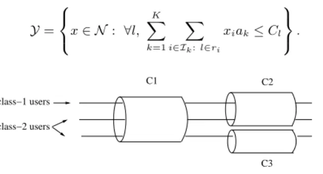
Consider for instance a cir-cuit switched network composed ofLlinks with respective capacitiesC1, . . . , CLand shared byKuser classes. Class-k users arrive at rate νk and require a circuit of capacity akfor a random duration of mean 1/µkthrough one of the routes ri, i ∈ Ik, where each route ri consists of a sub-set of the links {1, . . . , L}. This definesN types of users withI1∪. . .∪ IK ={1, . . . , N}. Such a circuit switched network can be represented by the above queueing system where each nodeicorresponds to type-iusers. If i∈ Ik, this corresponds to users that occupy a circuit of capacity akalong routeriduring a random duration of mean 1/µk. Specifically, the service rate of nodeiis given by:φi(x) =xiakµk, fori∈ Ik.
Thus the service rates are balanced with corresponding bal-ance function: Φ(x) = K Y k=1 Y i∈Ik 1 xi!axkiµ xi k .
The network capacity is determined by the link capacities:
Y= 8 < : x∈ N : ∀l, K X k=1 X i∈Ik:l∈ri xiak≤Cl 9 = ; . r1 r2 r3 class−2 users class−1 users C1 C2 C3
Figure 2: A network with 2 user classes
A typical example is a telephone network whereak= 1 for allkand the capacityClcorresponds to the number of available circuits on linkl. The example depicted in Figure 2 consists of K = 2 user classes where class-1 users can take route r1 = {1,2} only while class-2 users can take
either router2 ={1,2}or router3={1,3}. The network
capacity is given by:
Y={x∈ N : x1+x2+x3≤C1, x1+x2≤C2, x3≤C3}.
Data networks.
We now consider a data network com-posed ofLlinks with respective capacitiesC1, . . . , CL and shared byKuser classes. Class-kusers arrive at rateνkand require the transfer of a document of random size of mean 1/µk through one of the routesri,i∈ Ik. Again, this de-finesNtypes of users withI1∪. . .∪ IK ={1, . . . , N}. The duration of a data transfer depends on its bit rate. We as-sume that the overall bit rateγi(x) of type-iusers depends on the network statexonly and is equally shared between these users. Such a data network can be represented by the above queueing system where each nodeicorresponds to type-iusers, that transfer a document through routeri. The service rate of nodeiis:φi(x) =µkγi(x), i∈ Ik.
The allocation must satisfy the capacity constraints:
∀l, X
i:l∈ri
γi(x)≤Cl.
The balanced allocation for which at least one capacity con-straint is reached in any state is known as “balanced fair-ness” [3]. We have:
γi(x) =
Γ(x−ei)
Γ(x) , ∀x:xi>0,
where Γ is the positive function recursively defined by Γ(0) = 1 and: Γ(x) = max l 1 Cl X i:l∈ri,xi>0 Γ(x−ei).
The balance function Φ which characterizes the service rates of the corresponding queueing network is then given by:
Φ(x) = Γ(x) K Y k=1 Y i∈Ik 1 µxi k .
The network capacity can be determined so as to guarantee a minimum data rateγfor instance, in which case:
Y= x∈ N : ∀i, γi(x) xi ≥γ ff .
3.
A SINGLE CLASS
We first consider the caseK= 1. There is a single stream of incoming customers, that can be routed to any of theN network nodes. We first characterize the class of admissi-ble load balancings and then use this characterization to identify optimal strategies in terms of blocking probability.
3.1
Characterization
Denote byS ⊂ A the set of balance functions that cor-respond to “simple” load balancings in the sense that cus-tomers can be blocked in a single state. We denote by Λy the element ofS such that customers are blocked in state y∈ Y only. Proposition 1. We have: Λy(x) = Λy(y) |y−x| y−x ! 1 ν|y−x| ifx≤y,
andΛy(x) = 0otherwise. The constantΛy(y)is determined
by the normalizing conditionΛy(0) = 1.
Proof. For any statex≤y,x6=y, we have:
Λy(x) = 1 ν N X i=1 Λy(x+ei).
In particular, Λy(x) is equal to the product of Λy(y)/ν|y−x| by the number of direct paths fromxtoy. 2
The blocking probability associated with a simple load balancing can be easily evaluated using the following recur-sive formula:
Proposition 2. Let 1/δ(y) be the blocking probability
associated with the balance functionΛy∈ S. We have: δ(y) = 1 + N X i=1 φi(y) ν δ(y−ei),
withδ(0) = 1andδ(y) = 0for anyy6∈ N.
Proof. Using the identity:
|y−x| y−x ! = X i:yi>xi |y−x−ei| y−x−ei ! , x≤y, we deduce from (10) and Proposition 1 that: δ(y) = P x≤yπ(x) π(y) = 1 Φ(y) X x≤y Φ(x) |y−x| y−x ! 1 ν|y−x| = 1 + 1 Φ(y) X x≤y,x6=y X i:yi>xi Φ(x) |y−x−ei| y−x−ei ! 1 ν|y−x| = 1 + N X i=1 φi(y) ν × 1 Φ(y−ei) X x≤y−ei Φ(x) |y−x−ei| y−x−ei ! 1 ν|y−x−ei| = 1 + N X i=1 φi(y) ν δ(y−ei). 2
The following result characterizes the set of admissible balance functionsAas linear combinations of elements of
S:
Theorem 1. For any balance function Λ∈ A, we have:
Λ =X
y∈Y
α(y)Λy, (11)
where for ally∈ Y,
α(y) = β(y) Λy(y)
with β(y) = Λ(y)− 1
ν N
X
i=1
Λ(y+ei).
Conversely, for anyα∈ F such that P
y∈Yα(y) = 1, the
balance functionΛdefined by (11) lies inA.
Proof. In view of (8), there exists a function β ∈ F
such that for any statex: Λ(x) =β(x) + 1 ν N X i=1 Λ(x+ei). (12)
As Λ(x) = 0 for any statex6∈ Y, we deduce that Λ is in fact entirely determined by the function β through (12). The
proof of equality (11) then follows from the fact that the functionP
y∈Yα(y)Λysatisfies (12) in any statex∈ Y:
X y∈Y α(y)Λy(x) = α(x)Λx(x) + X y∈Y y≥x,y6=x α(y)Λy(x), = β(x) + X y∈Y y≥x,y6=x α(y)1 ν N X i=1 Λy(x+ei), = β(x) +1 ν N X i=1 X y∈Y α(y)Λy(x+ei). Conversely, any linear combination Λ = P
y∈Yα(y)Λy of elements ofS withP
y∈Yα(y) = 1 satisfies Λ(0) = 1,X ⊂
Y as well as inequalities (8). 2
3.2
Optimal load balancing
We deduce from Theorem 1 that there exists an optimal admissible load balancing which is simple. In particular, the state of actually attainable states X associated with this optimal solution is of the form{x∈ N :x≤y} and therefore generally smaller than the set of potentially at-tainable statesY.
Corollary 1. There is a balance functionΛ∈ S which
minimizes the blocking probability over the setA.
Proof. The blocking probability is given by:
p=X x∈X π(x) 1− N X i=1 λi(x) ν ! . In view of (5) and (10), we deduce:
p = P x∈Y(1− 1 ν PN i=1λi(x))Λ(x)Φ(x) P x∈YΛ(x)Φ(x) = P x∈Y(Λ(x)− 1 ν PN i=1Λ(x+ei))Φ(x) P x∈YΛ(x)Φ(x) . It then follows from Theorem 1 that
p= P y∈Yβ(y)Φ(y) P y∈Yβ(y)Ψ(y) with Ψ(y) =X x∈Y Λy(x) Λy(y) Φ(x), y∈ Y. In particular, p≥min y∈Y Φ(y) Ψ(y).
Let y? be a state where the function y 7→ Φ(y)/Ψ(y) is minimal. The blocking probabilitypis minimal ifβ(y) = 0 for ally∈ Yexcepty?. The corresponding balance function
is Λy?∈ S. 2
Remark 1. In view of Corollary 1 and Proposition 2,
finding the optimal admissible load balancing requiresO(|Y|)
operations only, where |Y|denotes the number of elements in the setY.
It is possible to further characterize the optimal load bal-ancing when the network is “monotonic” in the sense that: φi(x)≥φi(x−ej), ∀i, j, ∀x:xj>0. (13) We say that a statey ∈ Y is extremal if y+ei 6∈ Y for all i= 1, . . . , N. The following result is a consequence of Proposition 2:
Proposition 3. LetΛy∈ S be a balance function which
minimizes the blocking probability over the set A. If the network is monotonic,yis an extremal state of Y.
Proof. Let 1/δ(y) be the blocking probability
associ-ated with the balance function Λy ∈ S if y ∈ Y, and δ(y) = 0 otherwise. We prove by induction on|y|that:
∀y∈ Y, ∀j, δ(y)≥δ(y−ej).
The property holds fory= 0. Now assume that the prop-erty holds for ally∈ Ysuch that|y|=n, for some integern. Lety∈ Ysuch that|y|=n+ 1. It follows from Proposition 2 and the monotonicity property that:
∀j, δ(y) = 1 + N X i=1 φi(y) ν δ(y−ei), ≥ 1 + N X i=1 φi(y−ej) ν δ(y−ei−ej), = δ(y−ej).
Thusδ(y) is maximal for an extremal state ofY. 2
4.
SEVERAL CLASSES
When K ≥ 2, admissible load balancings can still be written as linear combinations of simple load balancings as in Theorem 1 but with additional constraints that cannot be simply characterized. Thus we restrict the analysis to the class of so-called “decentralized” load balancings where the routing decision for a class-kcustomer does not depend on the number of customers of other classes. This class presents the practical interest of requiring local information only, unlike the general class of admissible load balancings where the routing decisions are based on the overall network state.
4.1
Characterization
For any statex∈ N, we define the restricted statex(k)≡ P
i∈Ikxieigiving the number of class-kcustomers in each
nodei∈ Ik. LetN(k) ≡ {x(k), x∈ N }be the correspond-ing state space. We define the class of decentralized load balancings as those for which the corresponding balance function has the following product-form:
Λ(x) = K
Y
k=1
Λ(k)(x(k)) ifx∈ Y, Λ(x) = 0 otherwise,
where Λ(k) is the restriction of Λ to the setN(k). We
de-fineDas the set of balance functions Λ ∈ Ahaving such a product-form. Note that the load balancing is decentral-ized in the sense that the routing probability of a class-k
customer to each nodei∈ Ikis independent of the number of customers of other classes:
λi(x−ei) = Λ(x) Λ(x−ei) = Λ (k)(x(k)) Λ(k)(x(k)−ei), ∀x∈ Y: xi>0.
We now extend the notion of “simple” load balancing defined in§3.1. LetY(k)={x(k), x∈ Y}and:
Y0={x∈ N : ∀k, x(k)∈ Y(k)}.
ThusY0is the set of statesxsuch that any restricted state x(k) belongs toY. Note thatY0 containsY and is equal to
Y ifY={x∈ N : x≤y}for some statey. We now refer toS as the set of balance functions Λy, y∈ Y0, defined by:
Λy(x) = K
Y
k=1
Λy(k)(x(k)),
where Λy(k)(x(k)) is the simple load balancing for class-k customers as defined in §3.1. The following result is the analog of Theorem 1.
Theorem 2. For any balance function Λ∈ D, we have:
Λ(k)= X
y∈Y(k)
α(k)(y)Λy,
where for ally∈ Y(k),
α(k)(y) =β
(k)(y)
Λy(y)
with β(k)(y) = Λ(y)−1
νk
X
i∈Ik
Λ(y+ei).
In particular, we have for anyx∈ Y:
Λ(x) = X
y∈Y0
α(y)Λy(x),
where for ally∈ Y0, α(y) = β(y) Λy(y) with β(y) = K Y k=1 β(k)(y(k)).
Proof. We obtain the expressions for Λ(k) as in the
proof of Theorem 1. The proof then follows from the fact that for allx∈ Y:
Λ(x) = K Y k=1 Λ(k)(x(k)) = K Y k=1 X y∈Y(k) β(k)(y) Λy(y) Λy(x) = X y∈Y0 K Y k=1 β(k)(y(k)) Λy(k)(y(k)) Λy(k)(x(k)) = X y∈Y0 α(y)Λy(x). 2
4.2
Optimal load balancing
As in the case of a single class, we deduce from Theorem 2 that there exists an optimal admissible load balancing which is simple, for both the overall blocking probability and the maximum per-class blocking probability objectives.
Corollary 2. There is a balance functionΛ∈ Swhich
minimizes the overall blocking probability over the set D.
Proof. The overall blocking probability is given by:
p=X x∈X π(x) 1− N X i=1 λi(x) ν ! . In view of (5) and (10), we deduce:
p= 0 @ X x∈Y K X k=1 νk ν (Λ (k) (x(k))− 1 νk X i∈Ik Λ(k)(x(k)+ei)) × Y l6=k Λ(l)(x(l))Φ(x) 1 A/ X x∈Y Λ(x)Φ(x) ! . It then follows from Theorem 2 that
p=
P
y∈Y0β(y)Φ0(y)
P y∈Y0β(y)Ψ(y) , with Φ0(y) =X x∈Y K X k=1 νk ν × Y l6=k Λy(l)(x(l)) Λy(l)(y(l)) ×Φ(y(k)+X l6=k x(l)) and Ψ(y) =X x∈Y Λy(x) Λy(y) Φ(x), y∈ Y0. In particular, p≥min y∈Y0 Φ0(y) Ψ(y).
We conclude that the blocking probabilityp is minimal if β(y) = 0 for all y ∈ Y except for one statey? where the function y 7→Φ0(y)/Ψ(y) is minimal. The corresponding
balance function is Λy?∈ S. 2
Corollary 3. There is a balance functionΛ∈ Swhich
minimizes the maximum per-class blocking probability over the setD.
Proof. The blocking probability of class-kcustomers is
given by pk= X x∈X π(x) 0 @1− X i∈Ik λi(x) νk 1 A.
It then follows as in the proof of Corollary 2 that max
k=1,...,Kpk=
P
y∈Y0β(y)Φ00(y)
P y∈Y0β(y)Ψ(y) , with Φ00(y) = max k=1,...,K X x∈Y 1 νk ×Y l6=k Λy(l)(x(l)) Λy(l)(y(l)) ×Φ(y(k)+X l6=k x(l)) and Ψ(y) =X x∈Y Λy(x) Λy(y) Φ(x), y∈ Y0.
We conclude that the maximum per-class blocking proba-bility is minimal if β(y) = 0 for all y ∈ Y except for one state y? where the functiony 7→ Φ00(y)/Ψ(y) is minimal. The corresponding balance function is Λy?∈ S. 2
5.
EXAMPLES
We apply previous theoretical results to a reference sys-tem consisting of a set of parallel servers, with and without background traffic.
5.1
Absence of background traffic
We first considerNparallel servers fed by a single stream of customers, as illustrated in Figure 3. Such a system may represent a supercomputer center, for instance, or any other distributed server system. For communication networks, it might correspond to a logical link split over several physical links. In this case, we consider data traffic only as, for telephone traffic, any policy which blocks a call only when all circuits are occupied is obviously optimal.
server 2 server 1
server 3 customer arrivals
Figure 3: The reference system: a set of parallel servers.
The model is the same as that considered in [2]. De-note by x = (x1, . . . , xN) the network state, C1, . . . , CN the server capacities and 1/µthe mean service requirement. We have:
φi(x) =µCi, corresponding to the balance function:
Φ(x) = QN 1
i=1(µCi)xi
The network capacity region, defined so as to guarantee a minimum service rateγ, may be written:
Y={x:∀i, xi≤Ci/γ}. The overall system load is given by:
%= ν µ N X l=1 Ci .
The monotonicity property (13) trivially holds and it fol-lows from Corollary 1 and Proposition 3 that the optimal insensitive load balancing is characterized by the balance function: Λ(x) = |y−x| y−x ! / |y| y ! ×ν|x| ifx≤y, and Λ(x) = 0 otherwise, whereyis the vector such thatyi is the largest integer smaller thanCi/γ. In view of (5), the corresponding arrival rates are:
λi(x) =yi−xi
|y−x|ν, x≤y.
Viewing each serverias a resource ofyipotential “circuits” of rateγ, this boils down to routing new demands in pro-portion to the number of available circuits at each server.
0.0001 0.001 0.01 0.1 1 0.4 0.6 0.8 1 1.2 1.4 1.6 Blocking probabilty Overall load Greedy Best insensitive Best static 0.0001 0.001 0.01 0.1 1 0.4 0.6 0.8 1 1.2 1.4 1.6 Blocking probabilty Overall load Greedy Best insensitive Best static
Figure 4: Two parallel links with symmetric ca-pacities (upper graph) and asymmetric caca-pacities (lower graph).
We compare the resulting blocking probability with that obtained for the best static load balancing and the greedy load balancing, respectively. We refer to the greedy strat-egy as that where users are routed at timetto serveri(t) with the highest potential service rate :
i(t) = arg max
i=1,...,N
Ci xi(t−) + 1
. (14)
Note that for symmetric capacities, this is equivalent to joining the shortest queue. The greedy strategy is sensi-tive. Results are derived by simulation for i.i.d. exponential services.
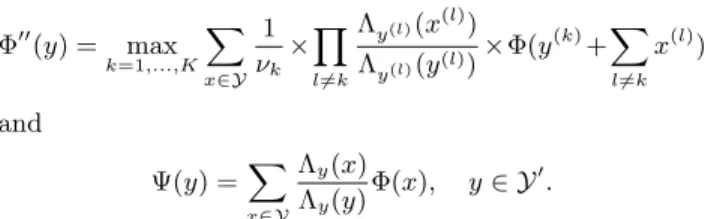
Figure 4 gives the blocking probability for two servers of symmetric capacities (C1=C2= 1) and asymmetric
capac-ities (C1= 1,C2= 0.5) withγ= 0.1. We observe that the
best insensitive load balancing provides a tight approxima-tion for the greedy strategy, which is known to be optimal for i.i.d. exponential services with the same mean (cf. Sec-tion 1). We verified by simulaSec-tion that, for both symmetric and asymmetric scenarios, the performance of the greedy strategy is in fact only slighty sensitive to the service re-quirement distribution and therefore that the above approx-imation remains accurate under general traffic assumptions.
5.2
Presence of background traffic
We now consider a set of N parallel servers as depicted in Figure 5, with a “flexible” stream corresponding to users that can be routed to either server, and one “background” stream per server corresponding to users whose route is fixed. This system withN = 2 servers is used in [16] for modeling a wireless telephone network with two overlapping cells: the flexible stream corresponds to those users in the overlapping area that can be served by either cell while each background stream corresponds to users that can be served by one cell only.
background traffic
background traffic flexible stream
server 2 server 1
Figure 5: Parallel servers with background traffic.
Let (x, x0) be the network state, wherex= (x
1, . . . , xN) andx0 = (x0
1, . . . , x0N) describe the number of users of the flexible and background streams, respectively. We denote byCithe capacity of serveriand byφi(x, x0) andφ0i(x, x0) the service rates of flexible and background users at server i, respectively. We here consider the two types of traffic described in§2.5:
• Telephone traffic, where each user requires a circuit of unit capacity. Denoting by 1/µthe mean call duration for a user of the flexible stream, 1/µi the mean call duration for a user of the background stream of server i, we get:
φi(x, x0) =xiµandφi0(x, x0) =x0iµi, for alli. This corresponds to the balance function:
Φ(x, x0) = 1 QN i=1xi!x0i!µxiµ x0 i l . The network capacity region is defined by:
• Data traffic, where the capacity of each link is fairly shared between active users. Denoting by 1/µ the mean document size for a user of the flexible stream, 1/µi the mean document size for a user of the back-ground stream of serveri, we get for alli:
φi(x, x0) = xi xi+x0i Ciµ and φ0i(x, x0) = x0 i xi+x0i Ciµi. This corresponds to the balance function:
Φ(x, x0) = N Y i=1 xi+x0i xi ! 1 Cxi+x0i i 1 µxiµx 0 i i . The network capacity region is characterized by a minimum data rateγ so that:
Y={(x, x0) :∀i, xi+x0i≤Ci/γ}.
Traffic parameters.
Letν be the arrival rate of the flexi-ble stream,νi the arrival rate of the background stream of serveri. The overall traffic intensity is given by:ρ= ν µ+ N X i=1 νi µi .
For telephone traffic, this is expressed in Erlangs and the capacity of each link corresponds to the number of avail-able circuits. For data traffic,ρand the link capacities are expressed in bits/s. The overall system load is defined as:
%= PNρ
i=1Ci
.
In the presence of background traffic, the optimal insensi-tive strategy depends on the traffic intensity. As shown in the following examples, it remains approximately the same for a large range of offered loads, however, indicating that a fixed strategy could be chosen in practice.
0 2 4 6 8 10 0 0.5 1 1.5 2
Maximum number of flexible customers
Overall load
Telephone traffic Data traffic
Figure 6: The best decentralized load balancing with homogeneous service requirements.
We consider N = 2 servers of the same capacity, C1 =
C2 = 10. Each background stream represents 10% of the
overall traffic intensity. The minimum data rate isγ= 1.
Homogeneous service requirements.
We first consider the case of homogeneous service requirements,µ=µ1=µ2.In view of Corollary 2, there is a simple load balancing, characterized by a state (y, y0) ∈ Y0, that minimizes the overall blocking rate over all decentralized insensitive load balancings. It turns out that y0 = (10,10) for all traffic loads, i.e., the corresponding balance function is:
Λ(x, x0) = |y−x| y−x ! / |y| y ! ×ν|x|νx01 1 ν x02 2 ifx≤y,
and Λ(x, x0) = 0 otherwise. Letnbe the maximum number of flexible users per link, i.e., y = (n, n). Figure 6 shows how n varies with respect to the system load % for both telephone and data traffic.
0.0001 0.001 0.01 0.1 1 0.4 0.6 0.8 1 1.2 1.4 1.6
Overall blocking probability
Overall load Greedy Best decentralized Best static 0.0001 0.001 0.01 0.1 1 0.4 0.6 0.8 1 1.2 1.4 1.6
Overall blocking probabilty
Overall load Greedy Best decentralized Best static
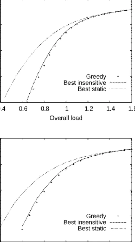
Figure 7: Overall blocking rate for telephone traffic (upper graph) and data traffic (lower graph) with homogeneous service requirements.
Figure 7 gives the resulting overall blocking probability. Results are compared with those of the best static load balancing and the greedy load balancing where a user is routed to that server where most resources are available.
Specifically, a user of the flexible stream arriving at time t is routed to that serveri(t) with the largest number of available circuits for telephone traffic:
i(t) = arg max
i=1,2Ci−xi(t
−)
−x0i(t −),
with the highest potential rate for data traffic: i(t) = arg max
i=1,2
Ci
xi(t−) +x0i(t−) + 1 .
Again, the greedy policy is sensitive and results are de-rived by simulation with i.i.d. exponential services in this case. We observe that the greedy load balancing outper-forms any other strategy for both telephone and data traf-fic. This strategy requires a complete knowledge of the net-work state, however, unlike the other two strategies. Note that the static load balancing is decentralized and insensi-tive, therefore leads to a higher blocking rate than the best decentralized insensitive strategy.
Heterogeneous service requirements.
We now consider the case of heterogeneous service requirements, namelyµ= µ1/100 = µ2/100. A strategy that minimizes the overallblocking probability would tend to block the flexible stream in view of the higher service requirements. Thus we rather consider the best decentralized load balancing in terms of the maximum per-class blocking rate. In view of Corol-lary 3, there is a simple load balancing that minimizes the maximum per-class blocking rate, characterized by a state (y, y0)∈ Y0. Again, we havey= (n, n) andy0= (10,10) for all traffic loads. Figure 8 shows hownvaries with respect to the system load%for both telephone and data traffic.
0 2 4 6 8 10 0 0.5 1 1.5 2
Maximum number of flexible customers
Overall load
Telephone traffic Data traffic
Figure 8: The best decentralized load balancing with heterogeneous service requirements.
Figure 9 gives the resulting maximum per-class block-ing probability compared with that of the best static load balancing and the greedy load balancing. We observe that the greedy load balancing in no longer the best strategy, especially at high loads. For data traffic at load%= 1 for instance, both the greedy strategy and the best static strat-egy lead to a blocking rate approximately equal to 10%, while the best insensitive strategy gives a blocking rate of 5%. 0.001 0.01 0.1 1 0.4 0.6 0.8 1 1.2 1.4 1.6
Maximum blocking probability
Overall load Greedy Best decentralized Best static 0.0001 0.001 0.01 0.1 1 0.4 0.6 0.8 1 1.2 1.4 1.6
Maximum blocking probabilty
Overall load Greedy Best decentralized Best static
Figure 9: Maximum per-class blocking rate for tele-phone traffic (upper graph) and data traffic (lower graph) with heterogeneous service requirements.
6.
CONCLUSION
While load balancing is a key component of computer systems and communication networks, most existing op-timality and performance results are derived for specific topologies and traffic characteristics. In this paper, we have focused on those strategies that areinsensitiveto the dis-tribution of service requirements, in the general setting of Whittle networks. We have characterized any insensitive load balancing as a linear combination of so-called “sim-ple” strategies, for both a single customer class and sev-eral customer classes with decentralized routing decisions. This characterization leads to simple optimality and per-formance results that were illustrated on toy examples.
While we focused on external routing decisions only, it would be interesting to extend these results to internal
routing decisions, where the successive nodes visited by a customer depend on the load of these nodes. This is the subject of future research.
REFERENCES
[1] M. Alanyali, B. Hajek, Analysis of simple algorithms for dynamic load balancing, Mathematics of
Operations Research 22-4 (1997) 840–871. [2] T. Bonald, A. Prouti`ere, Insensitivity in
processor-sharing networks, Performance Evaluation 49 (2002) 193–209.
[3] T. Bonald, A. Prouti`ere, Insensitive bandwidth sharing in data networks, Queueing Systems 44-1 (2003) 69–100.
[4] X. Chao, M. Miyazawa, R. F. Serfozo and H. Takada, Markov network processes with product form
stationary distributions, Queueing Systems 28 (1998) 377–401.
[5] J.W. Cohen, The multiple phase service network with generalized processor sharing, Acta Informatica 12 (1979) 245–284.
[6] M.B. Combe, O.J. Boxma, Optimization of static traffic allocation policies, Theoretical Computer Science 125 (1994) 17–43.
[7] A. Ephremides, P. Varaiya, J. Walrand, A simple dynamic routing problem, IEEE Transactions on Automatic control 25 (1980) 690–693.
[8] M. Harchol-Balter, M. Crovella, C. Murta, On choosing a task assignment policy for a distributed server system, IEEE journal of parallel and distributed computing 59 (1999) 204–228.
[9] A. Hordijk, G. Koole, On the assignment of customers to parallel queues, Probability in the Engineering and Informational Sciences 6 (1992) 495–511.
[10] F.P. Kelly, Blocking Probabilities in Large
Circuit-switched Networks, Adv. Applied Probability 18 (1986) 473–505.
[11] F.P. Kelly, Routing and capacities allocations in networks with trunk reservations. Mathematics of operations research 15 (1990) 771–793.
[12] F.P. Kelly, Network routing, Philosophical Transactions of the Royal Society A337 (1991) 343–367.
[13] F.P. Kelly, Loss Networks, Annals of Applied Probabilities 1-3 (1991) 319–378.
[14] F.P. Kelly, Bounds on the performance of dynamic routing schemes for highly connected networks, Mathematics of Operations Research 19 (1994) 1–20. [15] F.P. Kelly, Mathematical modelling of the Internet,
in: Mathematics Unlimited - 2001 and Beyond
(Editors B. Engquist and W. Schmid), Springer-Verlag, Berlin (2001) 685–702.
[16] J. van Leeuwaarden, S. Aalto, J. Virtamo, Load balancing in cellular networks using first policy iteration, Technical Report, Networking Laboratory, Helsinki University of Technology, 2001.
[17] D. Mitra, R.J. Gibbens, B.D. Huang, State
dependent routing on symmetric loss networks with trunk reservations, IEEE Transactions on
communications 41-2 (1993) 400–411.
[18] S. Nelakuditi, Adaptive proportional routing: a localized QoS routing approach, in: Proc. of IEEE Infocom, 2000.
[19] R. Nelson, T. Philips, An approximation for the mean response time for shortest queue routing with general interarrival and service times, Performance evaluation 17 (1993) 123–139.
[20] S. Oueslati-Boulahia, E. Oubagha, An approach to routing elastic flows, in: Proc. of ITC 16, 1999. [21] R. Serfozo,Introduction to stochastic networks,
Springer, 1999.
[22] P. Sparaggis, C. Cassandras, D. Towley, Optimal control of multiclass parallel service systems with and without state information, in: proc. of the 32nd Conference on Decision Control, San Antonio, 1993. [23] S. Stidham, Optimal control of admission to a
queueing system, IEEE Transactions on Automatic Control 30-8 (1985) 705–713.
[24] A.N. Tantawi and D. Towsley, Optimal static load balancing in distributed computer systems, Journal of the ACM 32-2 (1985) 445–465.
[25] D. Towsley, D. Panayotis, P. Sparaggis,
C. Cassandras, Optimal routing and buffer allocation for a class of finite capacity queueing systems, IEEE Trans. on Automatic Control 37-9 (1992) 1446–1451. [26] W. Whitt, Deciding which queue to join: some
counterexamples, Operations research 34-1 (1986) 226–244.
[27] W. Winston, Optimality of the shortest line discipline, Journal of Applied Probability 14 (1977) 181–189.